


1. Introduction
Hyper-redundant manipulators have a large or infinite degree of kinematic redundancy, making them suited for many inspection and operation tasks in highly constrained environment, [Reference Chirikjian and Burdick1, Reference Chirikjian and Burdick2] such as search and rescue in earthquake-stricken areas, [Reference Wolf, Brown, Casciola, Costa, Schwerin, Shamas and Choset3] undersea exploration, [Reference Tang, Zhang, Huang, Li, Chen, Song, Zhu and Gu4] and capturing [Reference Wan, Sun and Yuan5] and removing debris missions in space [Reference Zhang and Liu6, Reference Zhang, Liu, Feng, Liu and Ju7]. All these missions are inseparable from obstacle avoidance planning which is exactly what we discuss in this paper. In this study, our proposed obstacle avoidance algorithm is more suitable for space hyper-redundant manipulators which do not have the problem of insufficient joint torque as the number of the manipulators’ links increases. Only kinematic planning problems are considered. As for studies of dynamic coupling and control methods, related works can be found in refs. [Reference Mu, Liu, Xu, Lou and Liang8, Reference Rybus9]. Hereafter, we abbreviate the obstacle avoidance algorithm proposed in this paper as RRTSC (rapidly exploring random tree and shape control) algorithm. Figure 1 shows two typical space application scenarios of the RRTSC algorithm. In the upper half of Fig. 1, the space hyper-redundant manipulator enters into a satellite for maintenance tasks, and in the lower half of Fig. 1, the manipulator passes through a truss for inspection tasks. For more on-orbit tasks in space, please refer to the study in ref. [Reference Rybus9].
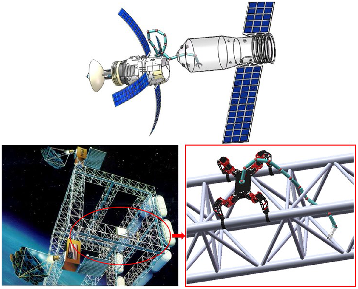
Figure 1. Application scenarios of the RRTSC algorithm.
Many studies have been presented to solve the obstacle avoidance issue for redundant manipulators. Among these works, the first group of works involves the use of Jacobian pseudo-inverse [Reference Marcos, Machado and Azevedo-Perdicoulis10, Reference Maciejewski and Klein11, Reference Qiu, Cao and Miao12, Reference Liao and Liu13, Reference Wan, Wu, Ma and Zhang14, Reference Ma and Nenchev15]. In this kind of method, the inverse kinematics solution of manipulators is expressed as a sum of a minimum-norm special solution and a general solution that contains an arbitrary vector. Assigning this vector according to some performance functions will not affect the pose of the manipulator’s end effector (the main task [Reference Marcos, Machado and Azevedo-Perdicoulis10]) but can adjust the configuration state of the intermediate links to complete some secondary tasks such as obstacle avoidance, [Reference Maciejewski and Klein11] singularity avoidance, [Reference Qiu, Cao and Miao12] joint physical limitation avoidance, [Reference Liao and Liu13, Reference Wan, Wu, Ma and Zhang14] and joint torque optimization [Reference Ma and Nenchev15]. In ref. [Reference Maciejewski and Klein11], a minimum distance point is detected between all links and obstacles at every instant and then an escaping velocity is applied to this critical point to ensure that all links do not collide with obstacles, while the end effector follows a given trajectory. However, the convergence rate of this pseudo-inverse-based approach will decrease rapidly owing to the fact that the increase of the number of links will lead to a huge calculation for Jacobian pseudo-inverse, which makes this kind of method unsuitable for hyper-redundant manipulators. The second group of works for obstacle avoidance planning of manipulators is developed by means of the artificial potential field [Reference Barraquand, Langlois and Latombe16, Reference Barraquand and Latombe17, Reference Conkur18]. In this kind of method, obstacles are represented by repulsive surfaces and the target point is represented by an attractive pole. The end effector of the manipulator is pulled by the potential field until it reaches the target point, and all links are repelled by obstacles to avoid collisions. This kind of method suffers from the problem that the manipulator may be trapped into local minima. In order to escape local minima, a randomized path planner is introduced to implement random steps in the local minima [Reference Barraquand, Langlois and Latombe16, Reference Barraquand and Latombe17]. However, this planner is implemented in configuration space (C-space) and is computationally expensive when utilized in high-dimensional cases. Additionally, in a complex obstacle environment with only narrow passages, the planner can hardly find a solution to escape the local minima. In ref. [Reference Conkur18], the harmonic function is utilized to construct a local minima-free potential field. The basic idea is to find a smooth path in the obstacle environment and develop a point settling algorithm to keep the tip of each link on this path until the manipulator reaches the target point. However, as the authors mentioned, this work will become considerably slow when extending it to a 3D calculation and it may fail to find a solution when an obstacle is located between the manipulator and the goal point. The third group of works for obstacle avoidance planning of manipulators involves searching in configuration space (C-space) [Reference Lozano-Perez19, Reference Kavraki, Svestka, Latombe and Overmars20, Reference Dasgupta, Gupta and Singla21, Reference Marcos, Machado and Azevedo-Perdicoulis22, Reference Zhao, Zhao and Liu23, Reference Ananthanarayanan and Ordez24, Reference Kuffner and Lavalle25, Reference Weghe, Ferguson and Srinivasa26, Reference Vahrenkamp, Berenson, Asfour, Kuffner and Dillmann27, Reference Shkolnik and Tedrake28, Reference Mesesan, Roa, Icer and Althoff29]. The concept of the C-space is first proposed in ref. [Reference Lozano-Perez19]. Two processes are needed in this study: a mapping process (or a C-space constructing process) and a searching process. The mapping process maps obstacles in Cartesian space to C-space, and this process is achieved by randomly selecting enough configurations (or angle sequences) of the manipulator and detecting whether the manipulator collides with obstacles in those configurations. The searching process is responsible for finding a feasible collision-free trajectory in the obtained C-space. However, it is not suitable for hyper-redundant manipulators because the high C-space dimension will cause a huge computational burden in the mapping process. An example of building a C-space can be found in ref. [Reference Maciejewski and Fox30]. The Probabilistic Roadmap Method (PRM), proposed in ref. [Reference Kavraki, Svestka, Latombe and Overmars20], replaces the mapping process [Reference Lozano-Perez19] with a learning process during which a graph is constructed. The graph is composed of nodes and edges, where the nodes correspond to collision-free configurations and the edges correspond to feasible trajectories. In ref. [Reference Dasgupta, Gupta and Singla21], a variational approach is presented to find a feasible collision-free solution after optimization, which takes the nodes of the graph in PRM as an initial guess. Indeed, PRM speeds up the searching process of feasible solutions to a certain extent. However, in order to improve the coverage of the graph in PRM to the C-space, considerable computer memory resources are needed as a guarantee. Some researchers use the Rapidly-exploring Random Tree (RRT) to find a feasible trajectory in C-space [Reference Kuffner and Lavalle25, Reference Weghe, Ferguson and Srinivasa26, Reference Vahrenkamp, Berenson, Asfour, Kuffner and Dillmann27, Reference Shkolnik and Tedrake28, Reference Mesesan, Roa, Icer and Althoff29]. The RRT has been widely utilized in the obstacle avoidance planning of mobile robots [Reference Wang, Meng and Khatib31]. When it is applied to manipulators, IK solver, [Reference Kuffner and Lavalle25] Jacobian pseudo-inverse, [Reference Vahrenkamp, Berenson, Asfour, Kuffner and Dillmann27, Reference Shkolnik and Tedrake28, Reference Mesesan, Roa, Icer and Althoff29] or Jacobian transpose [Reference Weghe, Ferguson and Srinivasa26] should be incorporated to improving the convergence rates of these RRT-based planners. In ref. [Reference Kuffner and Lavalle25], given a start point and a goal point in task space, corresponding to the start and goal configurations in C-space, obtained via an IK solver. The authors use an RRT-Connect path planner to establish a connection between the start and the goal configurations via a connect heuristic. If an IK solver is not available, the newly added node (or angle sequence) in C-space can be updated by an iterative process based on the Jacobian transpose [Reference Weghe, Ferguson and Srinivasa26] or Jacobian pseudo-inverse [Reference Vahrenkamp, Berenson, Asfour, Kuffner and Dillmann27, Reference Shkolnik and Tedrake28, Reference Mesesan, Roa, Icer and Althoff29]. During this iterative process, collision detections are executed to make sure that the newly added node is collision-free. These RRT-based planners can be utilized for pick-and-place tasks. [Reference Kuffner and Lavalle25, Reference Weghe, Ferguson and Srinivasa26, Reference Vahrenkamp, Berenson, Asfour, Kuffner and Dillmann27, Reference Shkolnik and Tedrake28] or end effector trajectory tracking tasks [Reference Mesesan, Roa, Icer and Althoff29]. It should be noted that the work in ref. [Reference Shkolnik and Tedrake28] executes RRT in task space to guide the search of a feasible trajectory in C-space and that the work in ref. [Reference Mesesan, Roa, Icer and Althoff29] executes RRT in both task space, guiding the end effector to follow a collision-free path in task space, and C-space, guiding the links not to collide with obstacles. However, in the case of hyper-redundant manipulators, the IK-solver may not be available and the calculations for Jacobian transpose or Jacobian pseudo-inverse will become inefficient. Some works utilize heuristic search algorithms such as genetic algorithm [Reference Marcos, Machado and Azevedo-Perdicoulis22] and ant colony optimization algorithm, [Reference Zhao, Zhao and Liu23] or multi-pass sequential localized search technique [Reference Ananthanarayanan and Ordez24] to find feasible solutions in C-space. However, the search processes in refs. [Reference Marcos, Machado and Azevedo-Perdicoulis22, Reference Zhao, Zhao and Liu23] are computationally inefficient and not suited for hyper-redundant manipulators. The work in ref. [Reference Ananthanarayanan and Ordez24] involves a process of discretizing the C-space and arranging them in ascending order, and this process will consume a lot of calculation time if the discretization accuracy is increased. The fourth group of works for obstacle avoidance planning of manipulators employs neural networks [Reference Zhang and Wang32, Reference Guo and Zhang33, Reference Guo and Zhang34]. In this kind of method, the inverse kinematics solution [Reference Hassan35, Reference Zhang, Zheng, Yu, Li and Yu36] and obstacle avoidance planning [Reference Zhang and Wang32, Reference Guo and Zhang33, Reference Guo and Zhang34] are incorporated as a quadratic programming (QP) formulation, which can be solved via neural networks. The inverse kinematics solution and obstacle avoidance are represented via a dynamic equality constraint and a dynamic inequality constraint, respectively. However, whether this kind of method can be applied to obstacle avoidance of hyper-redundant manipulators in a multi-obstacle environment, with high computational efficiency, is not mentioned.
The fifth and sixth groups of works for obstacle avoidance planning of manipulators are tractrix-based method [Reference Menon, Ravi and Ghosal37, Reference Ashwin, Chaudhury and Ghosal38] and backbone-curve-based method [Reference Chirikjian and Burdick39, Reference Choset and Henning40, Reference Fahimi, Ashrafiuon and Nataraj41, Reference Mu, Liu, Xu, Lou and Liang42, Reference Ma, Watanabe and Kondo43] (or shape control method called in this paper), respectively.The key idea of the tractrix-based method is that given the motion of a single link, the motion of all links of the manipulators can be obtained via an iteration process and a kinematics transformation from the first link to the end link. The motion of a single link is obtained via a tractrix curve. A single link consists of a leading end and a trailing end, and the leading end can track any 2D or 3D path in task space, while the trailing end follows the tractrix curve formulation, during which the link’s length remains unchanged. The tractrix-based method can be utilized to simulate the motion of one-dimensional flexible objects such as cables, ropes, ribbons, hair, and hyper-redundant manipulators in free space [Reference Sreenivasan, Goel and Ghosal44, Reference Menon, Ananthasuresh and Ghosal45, Reference Menon, Gurumoorthy and Ghosal46]. When the tractrix-based method is used in obstacle avoidance planning, optimization techniques must be incorporated to guide the trailing end of each link to escape away from the obstacles with a minimal energy cost. In ref. [Reference Menon, Ravi and Ghosal37], an optimization algorithm based on a calculus of variation is formulated where obstacles are modeled by smooth and differentiable super-ellipsoids. As for duct-type obstacles, the work in ref. [Reference Menon, Ravi and Ghosal37] suffers from a problem that analytical formulation of a duct is not always available. Therefore, the work in ref. [Reference Ashwin, Chaudhury and Ghosal38] proposes three representations of ducts. The basic idea of the backbone-curve-based method (or shape control method called in this paper) is employing a backbone curve to constrain the macro shape of a manipulator by fitting the curve and the manipulator’s shape as closely as possible [Reference Zhang, Liu, Ju and Yang47]. In essence, this kind of method reduces the planning dimension. The degrees of freedom of the manipulator are reduced to the number of parameters of the backbone curve, thus leading to a low computation cost and making it suitable for online path planning and real-time control of hyper-redundant manipulators. In ref. [Reference Chirikjian and Burdick39], “Tunnel” is defined in task space in which obstacles are present and then differential geometry is used to make the manipulator to be constrained to the tunnel. The tunnel (or backbone curve) is time-varying and collision-free with an ability to lead its endpoint to explore the obstacle space. However, although the tunnel (or backbone curve) is collision-free, it cannot guarantee that the manipulator is also collision-free unless the number of the links of the manipulator is so large that the manipulator’s shape can approximate the tunnel’s shape. On the other hand, the work in ref. [Reference Chirikjian and Burdick39] does not prescribe any strategy for constructing the tunnel and the tunnel is manually constructed [Reference Choset and Henning40]. To solve this problem, in ref. [Reference Choset and Henning40], a follow-the-leader approach is proposed and it adopts a roadmap technique, termed Generalized Voronoi Graph (GVG), to construct the tunnel. In ref. [Reference Fahimi, Ashrafiuon and Nataraj41], a harmonic potential function and a modified modal approach [Reference Fahimi, Asharafiuon and Nataraj48, Reference Chirikjian and Burdick1] are combined to construct the tunnel to constrain the macro shape of the manipulator. However, these approaches [Reference Choset and Henning40, Reference Fahimi, Ashrafiuon and Nataraj41, Reference Chirikjian and Burdick39] suffer from a common problem that the link model of the manipulator may collide with obstacles. Another interesting backbone-curve-based method is presented in ref. [Reference Mu, Liu, Xu, Lou and Liang42], with a novel modified modal approach [Reference Xu, Mu, Liu and Liang49]. In this work, the macro shape of the manipulator is constrained by the modified backbone curve. The even joint points of the manipulator are located on the curve, and the odd ones are released to accomplish the secondary tasks such as obstacle avoidance, by adjusting two kinds of parameters (the equivalent link length and angle between the adjacent equivalent links). However, the two kinds of parameters increase the solution dimension of the manipulator’s configuration, which deviates from the essence of the backbone-curve-based method. In other words, this work does not significantly reduce the planning dimension and will be computationally inefficient when dealing with obstacle avoidance of hyper-redundant manipulators in a highly constrained obstacle environment. Another interesting work is proposed in ref. [Reference Ma, Watanabe and Kondo43], in which a serpenoid curve is considered as the backbone curve to constrain the manipulator and then an obstacle mapping process in posture space is implemented, similar to a C-space construction. Although the mapping dimension is reduced to the parameter of the backbone curve, the mapping process will still cause a huge computation burden. In addition to the above six groups of methods, two other interesting works are shown in refs. [Reference Ananthanarayanan and Ordez50] and [Reference Xidias51]. In ref. [Reference Ananthanarayanan and Ordez50], a hybrid method combining analytical and numerical methods is proposed, in which the analytical equations are responsible for determining the first two and the last three joint angles, while the numerical technique is utilized for calculating the rest of the joints, and the obstacle avoidance is formulated as a constraint optimization problem and solved also by numerical techniques. In ref. [Reference Xidias51], a Hyper-BumpSurface is constructed to capture both the free and the forbidden areas of the environment as one mathematical entity, and then a genetic algorithm is employed to find a time-optimal trajectory in this hyper-surface. In summary, among the existing works, the backbone-curve-based method (or shape control method called in this paper) may be a good choice for dealing with obstacle avoidance of hyper-redundant manipulators in a highly constrained obstacle environment, without a huge computation burden. Our proposed RRTSC algorithm belongs to the category of the backbone-curve-based method.
The goal of this paper is to propose a kinematic obstacle avoidance planning algorithm for space hyper-redundant manipulators, in three-dimensional task space with static randomly distributed obstacles. Inspired by the works in refs. [Reference Choset and Henning40, Reference Fahimi, Ashrafiuon and Nataraj41] and aiming at solving the common problem (the backbone curve is collision-free, but the link model of the manipulator may collide with obstacles) existing in refs. [Reference Choset and Henning40, Reference Fahimi, Ashrafiuon and Nataraj41], we present the RRTSC algorithm. The successful implementation of the RRTSC algorithm is inseparable from a static curve, a dynamic time-varying backbone curve, and two novel shape control methods for these two curves. The task space is divided into two parts: obstacle space and free space. Correspondingly, the manipulator is divided into two parts: the inner part in the obstacle space and the outer part in the free space. The static curve and its corresponding shape control method are responsible for constraining the macro shape of the inner part of the manipulator and guiding it to move toward a goal point from a start point. The dynamic time-varying backbone curve and its corresponding shape control method are responsible for dynamically constraining the macro shape of the outer part of the manipulator. As time goes on, the inner part will be longer and the outer part will be shorter because the total number of links of the manipulator is constant. Please refer to Section 2.5 for details of how these two shape control methods are achieved. The main contributions of this study are summarized by the following remarks:
-
1. Different from the existing backbone-curve-based works [Reference Choset and Henning40, Reference Fahimi, Ashrafiuon and Nataraj41] in which only a dynamic backbone curve is constructed in real-time for constraining the macro shape of the manipulator, our proposed RRTSC algorithm combines a static curve and a dynamic backbone curve for the same purpose. To our best knowledge, it is the first attempt to accomplish obstacle avoidance of manipulators with a combination of a static curve and a dynamic backbone curve among existing works.
-
2. The existing backbone-curve-based works [Reference Choset and Henning40, Reference Fahimi, Ashrafiuon and Nataraj41] suffer from a common problem that the backbone curve is collision-free but the link model of the manipulator may collide with obstacles. Our proposed RRTSC algorithm does not have this problem. For a detailed comparison between our algorithm and existing works, please refer to Section 3.5.
-
3. The RRTSC obstacle avoidance algorithm architecture for hyper-redundant manipulators in three-dimensional space is proposed, including four components: a manual multi-sphere approximation for obstacles, an RRT algorithm, a dynamic backbone curve, and two novel shape control methods. Before the RRTSC algorithm is proposed, these four components are described. The implementation rules of the manual multi-sphere approximation for obstacles are discussed in detail. The RRT algorithm is employed to construct a static curve.
-
4. Novel shape control methods with the static curve and the dynamic backbone curve are proposed. Shape control with the static curve ensures that the manipulator in obstacle space is collision-free and guides the manipulator to move toward a goal point from a start point. Shape control with the dynamic backbone curve is responsible for constraining the macro shape of the manipulator in free space. It should be noted that the reason why we claim that the shape control method with the dynamic backbone curve is novel is based on the following two considerations. First, compared to the work in ref. [Reference Fahimi, Ashrafiuon and Nataraj41], we propose a more general form of the dynamic backbone curve. Second, we adopt a different way to solve the joint points of the manipulator. In ref. [Reference Fahimi, Ashrafiuon and Nataraj41], the joint points are solved by iteratively solving each joint point and every iteration is an optimization process. In this study, we fix some of the joint points on the dynamic backbone curve, and the remaining joint points are obtained through optimization processes, reducing the calculation time.
The remainder of this paper is organized as follows. Section 2 describes the main components of the RRTSC algorithm architecture, including the manual multi-sphere approximation for obstacles, the RRT algorithm, the dynamic backbone curve, and the two novel shape control methods. Section 2.1 introduces an overview of these components to facilitate readers to have a conceptual and holistic understanding of these components. The manual multi-sphere approximation for obstacles is discussed in Section 2.2. Section 2.3 reviews the RRT algorithm which will be later utilized to construct the static curve in obstacle space for the RRTSC algorithm. In Section 2.4, the dynamic time-varying backbone curve is constructed in a more general form compared to the one in ref. [Reference Fahimi, Ashrafiuon and Nataraj41]. Section 2.5 introduces the way to construct the static curve and proposes the two shape control methods (shape control with the static curve and shape control with the dynamic backbone curve). Shape control with the static curve is utilized to constraining the macro shape of the manipulator in obstacle space, while the shape control with the dynamic backbone curve is responsible for constraining the macro shape of the manipulator in free space. In Section 3, the RRTSC algorithm architecture is proposed and integrated simulations are carried out to demonstrate the feasibility of our algorithm. In addition, a comparison with existing works is also given in this section. Finally, the conclusions and future works are presented in Section 4.
2. RRTSC Algorithm Architecture
In this section, we first introduce the obstacle avoidance system model and then detail the components of the RRTSC algorithm separately.
2.1. System introduction
The whole obstacle avoidance system is illustrated in Fig. 2, and it is composed of obstacles, a rapidly exploring random tree (RRT), a RRT path, an environment boundary, a cubic spline interpolation curve, a backbone curve, and a hyper-redundant manipulator. Let us introduce them one by one. To facilitate reading, in Appendix part, all the symbols utilized in this paper are concluded in Tables A.1–A.4 and all the acronyms are summarized in Table A.5.
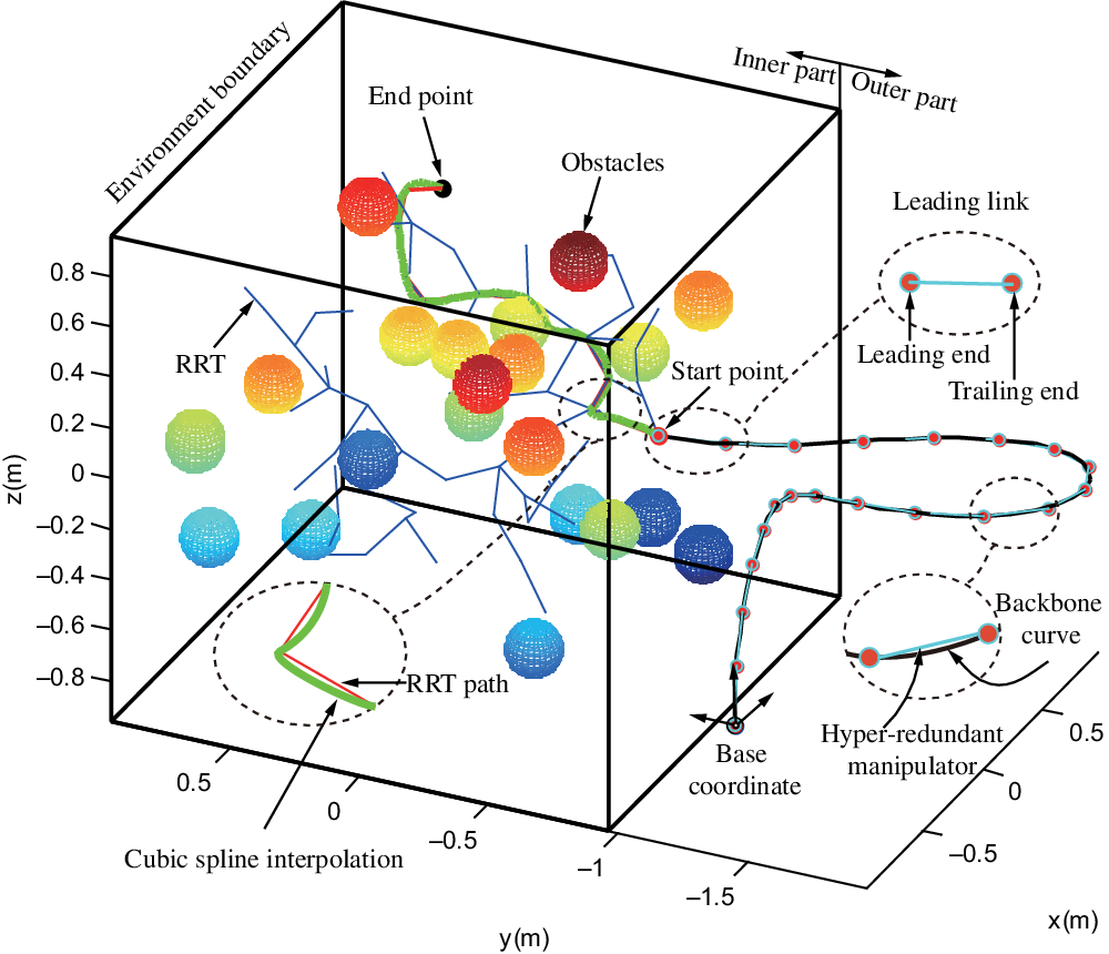
Fig. 2 Model of the whole obstacle avoidance system.
The obstacles are modeled by spheres in this case, and one sphere corresponds to one obstacle. However, an obstacle cannot be simply modeled via a sphere when the obstacle is a truss or a hole. To solve this problem, we adopt a manual multi-sphere approximation for obstacles in subsequent chapters. RRT algorithm [Reference Kuffner and Lavalle25] is a traditional path planning algorithm. The feature of this algorithm is that it can search high-dimensional space quickly and efficiently and guide the search to a blank area through random sampling points in a state space, so as to find a collision-free path from a starting point to a target point. As shown in Fig. 2, we use blue line segments to represent the RRT and red line segments to represent the collision-free RRT path. The start and end points of the RRT path are colored in red and black, respectively. The environment boundary is utilized to limit the sampling space of the RRT, and it is represented by a black rectangular external frame. It can be denoted by En_ limit = (X l , X r , Y l , Y r , Z l , Z r ), and the task space is divided into two parts: the inner part En_inner = {P|P ∈ En_limit} (or obstacle space) and the outer part En_outer = {P|P∉En_limit} (or free space), where P is any point in a 3D task space, and X l , X r , Y l , Y r , Z l , Z r are left and right limit coordinate values of the environment boundary. Considering that the RRT path is not a smooth curve, the cubic spline interpolation curve (green curve in Fig. 2) is adopted to replace the original RRT path. Define RRT_path and CSI_path to denote the RRT path and the cubic spline interpolation curve, respectively, for the convenience of describing pseudo codes in subsequent sections. The CSI_path is a smooth curve through a series of shape-value points which are RRT nodes in this study. The backbone curve, colored in black in Fig. 2, is constructed based on a modal approach, [Reference Chirikjian and Burdick1, Reference Fahimi, Asharafiuon and Nataraj48] and in this paper, it is extended to a more general form. The hyper-redundant manipulator is abstracted into cyan line segments connected end-to-end, and we refer to the line segments as the link model of the manipulator. The connection points represent joints colored in Indian red with three degrees of freedom. In this paper, we refer to the link where the end effector of the manipulator is located as the leading link. The leading link has two points. The end effector point is called the leading end, and the other is called the trailing end.

Fig. 3 Modeling for obstacles.
2.2. Modeling for obstacles
The choice of an approach to model obstacles usually is closely related to many factors, such as modeling accuracy, specific operation tasks, and principles of collision detection algorithms. Traditional obstacle modeling method commonly makes use of a sphere to model an obstacle with an irregular shape, and the sphere is located at the obstacle’s centroid with radius r = d
max, where d
max denotes the maximum distance from the centroid to envelope boundary. Figure 3(a) shows a cube obstacle, and Fig. 3(b), (c) illustrates the corresponding envelope sphere and the radius, respectively. For scenarios where the operation tasks are simple and require low modeling accuracy, it is wise to choose this method. However, when encountering the following situations where the tasks are passing through obstacles with holes (Fig. 3(d), (g)) or truss type obstacles (Fig. 3(j)), the traditional method will no longer work. Considering that, an alternative method for the representation of obstacles must be selected. An interesting method can be found in ref. [Reference Menon, Ravi and Ghosal37], in which obstacles are modeled using Minkowski sum [Reference Lozano-Perez19] (a combination or union of geometric entities) of differentiable super-ellipsoids [Reference Barr52]. The formulation of the super-ellipsoids contains five parameters, and by adjusting these parameters, a family of geometric entities, such as ellipses, rectangles, cylinders, spheres, etc., can be generated. Another interesting method [Reference Bradshaw and O’Sullivan53, Reference Stolpner, Kry and Siddiqi54] employs multi spheres to approximate geometric entities of arbitrary shape in an automatical way, and in our study, we refer to this method as the multi-sphere approximation method. Inspired by the works, [Reference Lozano-Perez19, Reference Bradshaw and O’Sullivan53, Reference Stolpner, Kry and Siddiqi54] we use the multi-sphere approximation method to represent obstacles. The representation in our study is implemented in a manual form for some simple geometric entities, considering that the manual representation can achieve better approximation accuracy with fewer spheres compared with the automatic one. It should be noted that the manual multi-sphere approximation has two main disadvantages: (1) It is not suitable for handling obstacles with complex shapes, since the manual discretization process will become difficult; (2) It is not suitable for large obstacle environments, since manual discretization process will become tedious. In addition, a lot of computer memory is needed to store the obstacles’ data. Therefore, for obstacles with complex shapes, the automatic multi-sphere approximation methods [Reference Bradshaw and O’Sullivan53, Reference Stolpner, Kry and Siddiqi54] are needed. For large obstacle environments, an algorithm can be developed to extract a local obstacle environment from a global one according to a specific task and then use the automatic multi-sphere approximation methods [Reference Bradshaw and O’Sullivan53, Reference Stolpner, Kry and Siddiqi54] in the local obstacle environment to obtain the spheres’ data. This algorithm essentially restricts the RRTSC algorithm to find a feasible solution in the local obstacle environment instead of the global one, which reduces the computational consumption to a certain extent. If this algorithm cannot be developed, we can also use other obstacle modeling methods. Our RRTSC algorithm does not rely on specific obstacle modeling methods. We model obstacles as multiple spheres to simplify the collision detection processes, in which only distance calculation from point to point is needed. In other words, other obstacle modeling methods, such as the super-ellipsoids method in ref. [Reference Menon, Ravi and Ghosal37], can also be integrated into our algorithm, as long as the three collision detection sub-algorithms in the RRTSC algorithm are appropriately modified. The way to envelope a geometric entity with spheres is similar to the principle of a 3D printer, which is traversing the spheres along the obstacle’s coordinate system. It is wise to choose different coordinate system types for different types of obstacles, as shown in Fig. 3(f) and (i) where the coordinate systems are chosen as Cartesian and cylindrical ones, respectively. The final envelope results are shown in Fig. 3(e) and (h). As for the envelope process, slice uniformly along the z -axis to obtain x − y (Fig. 3(f)) or
 $\theta$
− r (Fig. 3(i)) cross sections first, and then envelope the spheres along the cross-sectional curves until all cross sections along the z -axis are finished. In some special cases, the envelope method needs to be adjusted manually. Taking the truss-type obstacles (Fig. 3(j)) for illustration, the ultimate envelope result is shown in Fig. 3(k). The truss bars are considered as lines (Fig. 3(l)) instead of cylinders; therefore, it is not necessary to slice along the z -axis. It should be noted that the number and radius of the spheres must satisfy conditions that there are no gaps and at the same time guarantee suitable approximation accuracy. Figure 4 shows an example of how to implement a suitable approximation process in one- and two-dimensional spaces (three-dimensional space has a similar enveloping principle). r
env
represents the radius of a sphere. d
adj
denotes the distance between the centers of adjacent spheres. α
env
is the angle between two tangent lines at the intersection of adjacent circles (the cross section of the sphere is a circle). If d
adj
> 2r
env
, as shown in Fig. 4(a), there will be gaps among the spheres both in one- and two-dimensional spaces, which is a poor approximation case and will lead to a false obstacle avoidance detection. If d
adj
= 2r
env
, α
env
= 0°, as shown in Fig. 4(b), there is no gap in one-dimensional space but there is a gap in two-dimensional space. If d
adj
< 2r
env
, α
env
= 90°, as shown in Fig. 4(c), there is no gap whether in one- or two-dimensional space and it is a perfect approximation process. If d
adj
< 2r
env
, α
env
> 90°, as shown in Fig. 4(d), although the gap disappears, a phenomenon of over-approximation appears. For some complex geometry, this phenomenon is inevitable and what we need to do is to avoid it as far as possible. Compared with Fig. 4(c), r
env
in Fig. 4(d) increases, which leads to the decrease of approximation accuracy. In summary, the approximation process is based on a coordinate system and should choose the proper radius and number of the spheres and consider modeling accuracy, without affecting specific tasks.
$\theta$
− r (Fig. 3(i)) cross sections first, and then envelope the spheres along the cross-sectional curves until all cross sections along the z -axis are finished. In some special cases, the envelope method needs to be adjusted manually. Taking the truss-type obstacles (Fig. 3(j)) for illustration, the ultimate envelope result is shown in Fig. 3(k). The truss bars are considered as lines (Fig. 3(l)) instead of cylinders; therefore, it is not necessary to slice along the z -axis. It should be noted that the number and radius of the spheres must satisfy conditions that there are no gaps and at the same time guarantee suitable approximation accuracy. Figure 4 shows an example of how to implement a suitable approximation process in one- and two-dimensional spaces (three-dimensional space has a similar enveloping principle). r
env
represents the radius of a sphere. d
adj
denotes the distance between the centers of adjacent spheres. α
env
is the angle between two tangent lines at the intersection of adjacent circles (the cross section of the sphere is a circle). If d
adj
> 2r
env
, as shown in Fig. 4(a), there will be gaps among the spheres both in one- and two-dimensional spaces, which is a poor approximation case and will lead to a false obstacle avoidance detection. If d
adj
= 2r
env
, α
env
= 0°, as shown in Fig. 4(b), there is no gap in one-dimensional space but there is a gap in two-dimensional space. If d
adj
< 2r
env
, α
env
= 90°, as shown in Fig. 4(c), there is no gap whether in one- or two-dimensional space and it is a perfect approximation process. If d
adj
< 2r
env
, α
env
> 90°, as shown in Fig. 4(d), although the gap disappears, a phenomenon of over-approximation appears. For some complex geometry, this phenomenon is inevitable and what we need to do is to avoid it as far as possible. Compared with Fig. 4(c), r
env
in Fig. 4(d) increases, which leads to the decrease of approximation accuracy. In summary, the approximation process is based on a coordinate system and should choose the proper radius and number of the spheres and consider modeling accuracy, without affecting specific tasks.
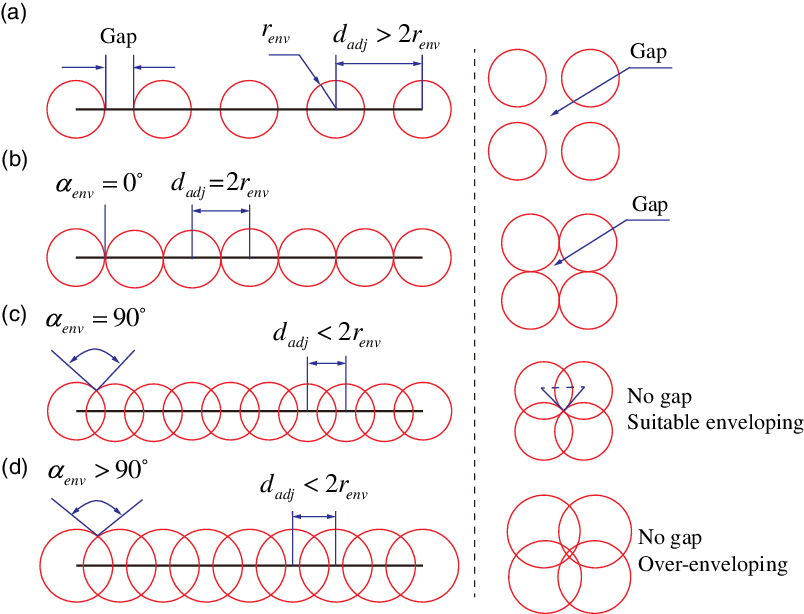
Fig. 4 Illustration example of how to implement a suitable approximation process.
2.3. RRT algorithm
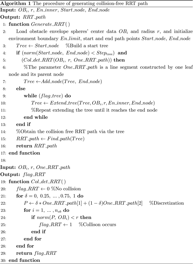
RRT algorithm [Reference Kuffner and Lavalle25] is an efficient obstacle avoidance planning method. The basic RRT algorithm is shown in Algorithm 1, and its relevant concept is shown in Fig. 5(a).
In Algorithm 1, the start tree Tree contains only one node during initialization. First, check if the start point Start_node and the target point End_node can be directly connected (lines 4 and 5). This should satisfy two conditions: (1) Distance between these two points is less than a given step threshold Step tree ; (2) The line segment One_RRT_path between these two points dose not collide with obstacles. If the conditions are met, add End_node to Tree, and if not repeat extending new nodes use function Extend_tree() (line 10) until Tree reaches End_node. The procedure of function Extend_tree() is not detailed in the above pseudo code, and we describe it as follows: (1) A sample function randomly selects a rand point Rand_node from the inner part of the obstacle environment En_inner; (2) A nearest function selects a node Nearst_node closest to Rand_node; (3) Extend a distance Step tree from Rand_node to Nearst_node and obtain One_RRT_path; (4) If a collision occurs, go to step 1, and if not add a new node New_node and check whether New_node could be directly connected to End_node; (5) Use flag variable flag_tree to denote whether Tree reaches the End_node. When a Tree is available, use function Find_path() to find a collision-free path RRT_path from the end point to the start point, with the help of index relationship between a leaf node and its parent node. It should be noted that Col_ det_RRT() detects collision every time a rand node is generated (lines 19–30). Principle of this function is easy to understand. First, discretize the line segment One_RRT_path via a coefficient vector Δ = (0, 0.25, 0.5, 0.75, 1) to get point set {P 1, P 2, P 3, P 4, P 5}, and then calculate the distance between OB i and P j , for i = 1, …, n ob where n ob is the number of spheres and j = 1, …, 5. If the distance is less than the sphere radius r, a collision has occurred and that means the Rand_node must be dropped.
Given a 3D task space where sphere obstacles are randomly distributed, initialize related parameters and execute the RRT algorithm, and we can obtain a tree shown in Fig. 5(b). The specific parameters will be detailed in Section 3. Different from traditional method which utilize RRT algorithm in C-space, [Reference Lozano-Perez19] our obstacle avoidance algorithm applies it in task space. There is an example for illustrating the differences between them. Figure 5(c) depicts a two-degree-of-freedom robotic arm, with two obstacles OB1 and OB2 surrounding it, in a plane task space. The corresponding representation of obstacles in C space, illustrated in Fig. 5(d), is obtained by a mapping process. This process can be described as two steps: (1) Change the joint angles
 $\theta$
1 and
$\theta$
1 and
 $\theta$
2 to get every possible configuration via forward kinematics; (2) Detect collision between the links and the obstacles to divide the C-space into obstacle area and non-obstacle area. Obviously, this process will become more difficult as the degrees of freedom of manipulators and the number of obstacles increase. To avoid this problem, we propose the RRTSC algorithm, using the RRT algorithm in task space and two shape control methods to drive a hyper-redundant manipulator. The two shape control methods use shape control curve to constrain the macro shape of a manipulator as shown in Fig. 5(e), and we will describe these two methods in Section 2.5.
$\theta$
2 to get every possible configuration via forward kinematics; (2) Detect collision between the links and the obstacles to divide the C-space into obstacle area and non-obstacle area. Obviously, this process will become more difficult as the degrees of freedom of manipulators and the number of obstacles increase. To avoid this problem, we propose the RRTSC algorithm, using the RRT algorithm in task space and two shape control methods to drive a hyper-redundant manipulator. The two shape control methods use shape control curve to constrain the macro shape of a manipulator as shown in Fig. 5(e), and we will describe these two methods in Section 2.5.

Fig. 5 Relevant illustration of RRT algorithm.
2.4. Backbone curve
As mentioned before, the backbone curve is employed to constrain the macro shape of a manipulator in En_ outer. This curve is a kind of spatial curve and its mathematical expressions are defined [Reference Fahimi, Asharafiuon and Nataraj48] as follows:
 \begin{equation}P(s,t) = {P_{{\rm{int}}}}(t) + \int_0^s {l(t) F(\sigma ,t)d\sigma }\end{equation}
where P(s, t), shown in Fig. 6(a), denotes an arbitrary point on the backbone curve. P
int
(t) is the initial point of the backbone curve in base frame, and it is defined as
 ${P_{{\rm{int}}}}(t) = {[{x_{{\rm{int}}}},{y_{{\rm{int}}}},{z_{{\rm{int}}}}]^{{T}}}$
. s and t are independent variables, representing arc length of the backbone curve and time, respectively. l(t) indicates the total length of the backbone curve at time t. F(
${P_{{\rm{int}}}}(t) = {[{x_{{\rm{int}}}},{y_{{\rm{int}}}},{z_{{\rm{int}}}}]^{{T}}}$
. s and t are independent variables, representing arc length of the backbone curve and time, respectively. l(t) indicates the total length of the backbone curve at time t. F(
 $\sigma$
, t) represents the unit vector tangent to the backbone curve at s =
$\sigma$
, t) represents the unit vector tangent to the backbone curve at s =
 $\sigma$
. Detailed representation of the backbone curve can be defined as follows:
$\sigma$
. Detailed representation of the backbone curve can be defined as follows:
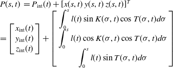 \begin{equation}\begin{array}{l}P(s,t)\; = {P_{{\rm{int}}}}(t) + {[x(s,t)\;y(s,t)\;z(s,t)]^{{T}}}\\= \left[ {\begin{array}{*{20}{c}}{{x_{{\mathop{\textrm{int}}} }}}(t)\\{{y_{{\mathop{\textrm{int}}} }}}(t)\\{{z_{{\mathop{\textrm{int}}} }}}(t)\end{array}} \right] + \left[ {\begin{array}{*{20}{c}}{\displaystyle \int_0^s {l(t)\sin K(\sigma ,t)\cos T(\sigma ,t)d\sigma } }\\{\displaystyle \int_0^s {l(t)\cos K(\sigma ,t)\cos T(\sigma ,t)d\sigma } }\\{\displaystyle \int_0^s {l(t)\sin T(\sigma ,t)d\sigma } }\end{array}} \right]\end{array}\end{equation}
Fig. 6 The backbone curve.
where K(
 $\sigma$
, t) is the angle between F
′(
$\sigma$
, t) is the angle between F
′(
 $\sigma$
, t) and y aixs of the base frame at s =
$\sigma$
, t) and y aixs of the base frame at s =
 $\sigma$
, and T(
$\sigma$
, and T(
 $\sigma$
, t) is the angle between F
′(
$\sigma$
, t) is the angle between F
′(
 $\sigma$
, t) and F(
$\sigma$
, t) and F(
 $\sigma$
, t) at s =
$\sigma$
, t) at s =
 $\sigma$
. Their geometric interpretation can be found in Fig. 6(b). The F
′ (
$\sigma$
. Their geometric interpretation can be found in Fig. 6(b). The F
′ (
 $\sigma$
, t) is the projection vector of F(
$\sigma$
, t) is the projection vector of F(
 $\sigma$
, t) on x − y plane on the base frame. If functions K(
$\sigma$
, t) on x − y plane on the base frame. If functions K(
 $\cdot$
) and T(
$\cdot$
) and T(
 $\cdot$
) are specified, P(s, t) can be obtained using Eq. (2). In ref. [Reference Chirikjian and Burdick1], K(
$\cdot$
) are specified, P(s, t) can be obtained using Eq. (2). In ref. [Reference Chirikjian and Burdick1], K(
 $\cdot$
) and T(
$\cdot$
) and T(
 $\cdot$
) are formulated as follows:
$\cdot$
) are formulated as follows:
 \begin{equation}\begin{array}{l}K(s,t){{ = }}\sum\limits_{i = 1}^{{n_1}} {{c_i}(t)} {f_i}(s)\\T(s,t){{ = }}\sum\limits_{i = 1}^{{n_2}} {{d_i}(t)} {g_i}(s)\end{array}\end{equation}
where f i (s) and g i (s) are mode functions, c i (t) and d i (t) are modal participation factors, n 1 is the number of mode functions for K(s, t), and n 2 is the number of mode functions for T(s, t). From the existing works, [Reference Chirikjian and Burdick1,Reference Fahimi, Ashrafiuon and Nataraj41] trigonometric functions are often used as the mode functions and the choice of them must meet two conditions. First, the trigonometric functions must be linearly independent. Otherwise, some participation factors will be lost. Second, the trigonometric functions cannot be all odd functions on the interval s ∈ [0, 1]. Otherwise, the backbone will be degenerated because the values of x and z for P(s, t) will always be equal to zero. According to these rules, the trigonometric functions can be chosen manually. It should be noted that n 1 + n 2 is the total number of mode functions, and this number should equal or exceed the number of constraints imposed on the backbone curve. In a 3D task space without obstacles, a total of seven constraints need to be satisfied, which means n 1 + n 2 is at least equal to seven. Three of the constraints are imposed by the position of the end point of the curve, and the remaining four constraints come from the intention of controlling the orientation at the start and end points of the curve. Now, we rewrite Eq. (3) into the following form:
 \begin{equation}\begin{array}{l}K(s,t) = {a_1}(t){f_1}(s) + {a_2}(t){f_2}(s) + {b_1}(t){f_3}(s) + {b_2}(t){f_4}(s)\\T(s,t) = {a_3}(t){g_1}(s) + {b_3}(t){g_2}(s) + {b_4}(t){g_3}(x)\end{array}\end{equation}
where a 1(t), a 2(t), a 3(t), b 1(t), b 2(t), b 3(t), and b 4(t) are participation factors. We hope that the orientation at the start and end points of the curve can be adjusted via intuitively adjusting one or a combination of the four parameters b 1(t), b 2(t), b 3(t), and b 4(t). Indeed, this can be achieved via a suitable selection of the mode functions. A specific example can be found in ref. [Reference Fahimi, Ashrafiuon and Nataraj41], where K(s, t) and T(s, t) are specified as follows:
 \begin{align}K(s,t) & = {a_1}(t)\sin (2\pi s) + {a_2}(t)(1 - \cos (2\pi s)) \nonumber\\ & \quad + {b_1}(t)\sin (\pi s/2) + {b_2}(t)(1 - \sin (\pi s/2))\\ T(s,t) & = {a_3}(t)(1 - \cos (2\pi s)) + {b_3}(t)\sin (\pi s/2) \nonumber\\ & \quad + {b_4}(t)(1 - \sin (\pi s/2))\nonumber\end{align}
where {b 1(t), b 3(t)} = {K(0, t), T(0, t)} and {b 2(t), b 4(t)} = {K(1, t), T(1, t)} specify the orientation at the start and end points of the backbone curve, respectively. In fact, the formulations for K(s, t) and T(s, t) are not unique and can be replaced by other ones. Considering that, we extend the formulations for K(s, t) and T(s, t) to a more general form. In other words, we give a selection rule for the mode functions. In Eq. (4), we make {b 1(t), b 3(t)} equal to {K(0, t), T(0, t)} and {b 2(t), b 4(t)} equal to {K(1, t), T(1, t)}, and then the selection rule for the mode functions is given as follows:
 \begin{equation}\left\{ {\begin{array}{l}{{f_1}(0) = {f_2}(0) = {f_4}(0) = 0,\;\;{f_3}(0) = 1}\\{{g_1}(0) = {g_3}(0) = 0,\;\;{g_2}(0) = 1}\\{{f_1}(1) = {f_2}(1) = {f_3}(1) = 0,\;\;{f_4}(1) = 1}\\{{g_1}(1) = {g_2}(1) = 0,\;\;{g_3}(1) = 1}\end{array}} \right.\end{equation}
In addition, the f 1(s), f 2(s), f 3(s), and f 4(s) must be linearly independent trigonometric functions and not all odd functions, the same as the g 1(s), g 2(s), and g 3(s). By now, the backbone curve is determined via parameters P int, l(t), a 1(t), a 2(t), a 3(t), b 1(t), b 2(t), b 3(t), and b 4(t) and we will put them into use in subsequent sections. It should be pointed out that in the follow-up simulations, we will use Eq. (5) to construct the dynamic backbone curve.
2.5. Shape control method
The shape control method is utilized to build rules of how to drive a hyper-redundant manipulator to move with a curve. We divide shape control into two categories: (1) Shape control with a static curve; (2) Shape control with a dynamic curve. As mentioned in Sections 2.3 and 2.4, we select the RRT path and the backbone curve to control the inner part and the outer part of a manipulator, respectively. The RRT path belongs to the static curve, whereas the backbone curve is one of the dynamic curves. The successful implementation of the RRTSC algorithm will use these two shape control methods. Now we will describe them, respectively.
2.5.1. Shape control with the dynamic backbone curve
First, let us describe the shape control method with the dynamic backbone curve. Assuming that a hyper-redundant manipulator is composed of links with length l link and number n link . Then, we can simplify the manipulator into line segments connected end to end, which is called the link model. The purpose of the shape control for the backbone curve is to calculate all connecting points (joint points), referred as P i for i = 0, …, n link , of the link model. It can be formulated as the following optimization problem:
 \begin{equation} {\rm{Solve}}:\;{P_i},\;\;\;\;i = 0,\;...\;,{n_{{\rm{link}}}}\end{equation}
 \begin{equation} {\rm{Minimize}}:\;\sum\limits_{i = 0}^{i = {n_{\rm{link}}}} {\left\| {\;{P_i} - {{P'}_i}\;} \right\|} ,\;\;\;\;i = 0,...\;,{n_{{\rm{link}}}}\end{equation}
 \begin{align}{\text{Subject to}}:{l_{{\rm{link}}}}\; &- eps \le \left\| {\;{P_i} - {P_{i - 1}}\;} \right\| \le {l_{{\rm{link}}}} + eps,\nonumber\\ & i = 0,...\;,{n_{{\rm{link}}}}\end{align}
where eps is a coefficient used to adjust the matching accuracy of the link length l
link
;
 ${P_i}^{\prime} $
denotes a equally spaced point on the backbone curve, and it satisfies Eq. (10).
${P_i}^{\prime} $
denotes a equally spaced point on the backbone curve, and it satisfies Eq. (10).
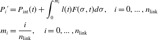 \begin{align}{P_i}^{\prime} & = {P_{{\rm{int}}}}(t) + \displaystyle \int_0^{{m_i}} {l(t)F(\sigma ,t)} d\sigma ,\;\;\;\;i = 0,...\;,{n_{{\rm{link}}}} \nonumber\\ {m_i} &= \displaystyle \frac{i}{{{n_{{\rm{link}}}}}},\;\;\;\;\;i = 0,...\;,{n_{{\rm{link}}}}\end{align}
 \begin{equation}{\rm{Solve}} :\;{P_i},\;\;i = 1,3,\;...\;,{n_{{\rm{link}}}} - 1\;({\rm{if}}\;{n_{{\rm{link}}}}\;{\rm{is}}\;{\rm{even}})\end{equation}
 \begin{equation}{\rm{Minimize}} :\;\left\| {\;{P_i} - {{P'}_i}\;} \right\|,\;\;i = 1,3,\;...\;,{n_{{\rm{link}}}} - 1\\\end{equation}
Subject to :
 \begin{equation}\left\{ {\begin{array}{l}{{P_i} = {P_i}^{\prime} ,\;\;i = 0,2,4,\;...\;,{n_{\rm{link}}}}\\{l_{{\rm{link}}}}\; - eps \le \left\| {\;{P_i} - {P_{i - 1}}\;} \right\| \le {l_{{\rm{link}}}} + eps,\;\;\\\;\;\;\;\;\;\;\;\;\;\;\;\;\;\;\:i = 1,3,\;...\;,{n_{{\rm{link}}}} - 1\end{array}} \right.\end{equation}
Equation (8) guarantees that P
i
is as close as possible to the backbone curve. In order to solve this optimization problem, let some
 ${P_i}^{\prime} $
equal
${P_i}^{\prime} $
equal
 ${P_i}^{\prime} $
(i =0, …, n
link
), then Eqs. (7)–(9) are reduced to Eqs. (11)–(13) if n
link
is even, or Eqs. (14)–(17) if n
link
is odd.
${P_i}^{\prime} $
(i =0, …, n
link
), then Eqs. (7)–(9) are reduced to Eqs. (11)–(13) if n
link
is even, or Eqs. (14)–(17) if n
link
is odd.
 \begin{align}{\rm{Solve}} :\;{P_i},\;\;i = 2,4,\;...\;,{n_{\rm{link}}} - 1\;({\rm{if}}\;{n_{{\rm{link}}}}\;{\rm{is}}\;{\rm{odd}}) \end{align}
 \begin{align} {\rm{Minimize}} :\;\left\| {\;{P_i} - {{P'}_i}\;} \right\|,\;\;i = 2,4,\;...\;,{n_{\rm{link}}} - 1 \end{align}
Subject to :
 \begin{equation}\left\{ {\begin{array}{l}{{P_i} = {P_i}^{\prime} ,\;\;\;\;i = 0}\\{{P_i} = {P_i}^{\prime} ,\;\;\;\;i = 1,3,\;...\;,{n_{{\rm{link}}}}}\\{l_{{\rm{link}}}}\; - eps \le \left\| {\;{P_i} - {P_{i - 1}}\;} \right\| \le {l_{{\rm{link}}}} + eps,\;\;\;\;\\\;\;\;\;\;\;\;\;\;\;\;\;\;\;i = 2,4,\;...\;,{n_{\rm{link}}} - 1\end{array}} \right.\end{equation}
The first lines of Eqs. (13) and (16) specify that P
i
|
i=0 (manipulator’s base) coincides with the start point of the backbone curve. The second line of Eq. (13) and the second line of Eq. (16) specify which points of P
i
are equal to
 ${P_i}^{\prime} $
, for i = 0, …, n
link
, and make
${P_i}^{\prime} $
, for i = 0, …, n
link
, and make
 ${P_i}{{{|}}_{i = {n_{{\rm{link}}}}}}$
(manipulator’s end effector) coincides with the end point of the backbone curve. According to Eqs. (11)–(16), employ mature optimization algorithms such as simulated annealing or particle swarm algorithm, and then we can easily get all the values of P
i
, for i = 0, …, n
link
. Figure 7(a) and (b) shows two shape control examples where n
link
= 4 and n
link
= 3, respectively. It can be seen that no matter n
link
is even or odd, the start and the end points always satisfy
${P_i}{{{|}}_{i = {n_{{\rm{link}}}}}}$
(manipulator’s end effector) coincides with the end point of the backbone curve. According to Eqs. (11)–(16), employ mature optimization algorithms such as simulated annealing or particle swarm algorithm, and then we can easily get all the values of P
i
, for i = 0, …, n
link
. Figure 7(a) and (b) shows two shape control examples where n
link
= 4 and n
link
= 3, respectively. It can be seen that no matter n
link
is even or odd, the start and the end points always satisfy
 ${P_0} = {P'_0}$
and
${P_0} = {P'_0}$
and
 ${P_{{n_{{\rm{link}}}}}} = {P'_{{n_{{\rm{link}}}}}}$
, which is realistic.
${P_{{n_{{\rm{link}}}}}} = {P'_{{n_{{\rm{link}}}}}}$
, which is realistic.

Fig. 7 Shapecontrol method.
In order to drive the manipulator to move, what we need to do is just changing the shape of the backbone curve by adjusting its parameters. Given a target point P target , an initial point P int (t), total arc length l(t), coefficients b 1(t), b 2(t), b 3(t), b 4(t), solve Eq. (17) via numerical approximation in Matlab, and then we can obtain parameters a 1(t), a 2(t), a 3(t).
 \begin{equation}{P_{{\rm{target}}}} = {P_{{\mathop{\textrm{int}}} }} + \int_0^1 {l(t)F(\sigma ,t) d\sigma }\end{equation}
If we replace P
target
with a continuous space curve, the manipulator will move continuously. Supplementary material shape_control_dscb_curve.mp4 shows an animation where the end effector of the manipulator and the corresponding end point of the backbone curve follow a given trajectory (“SIA”). Essentially, this is a process of constantly seeking inverse solutions. The label 7 in Fig. 7(c) is the “SIA” end trajectory, and P
target
is selected from it. Figure 7(c) depicts six backbone curves with different parameters listed in Table I, and the initial points are set as
 ${P_{{\mathop{\textrm{int}}} }} = {[0,0,0]^{{T}}}$
. For curves 1 and 2, target points are set as
${P_{{\mathop{\textrm{int}}} }} = {[0,0,0]^{{T}}}$
. For curves 1 and 2, target points are set as
 ${P_{{\mathop{\textrm{target}}} }} = {[0.15,0.54,0.30]^{{T}}}$
. For curves 3 and 4, target points are set as
${P_{{\mathop{\textrm{target}}} }} = {[0.15,0.54,0.30]^{{T}}}$
. For curves 3 and 4, target points are set as
 ${P_{{\mathop{\textrm{target}}} }} = {[0.50,0.52,0.30]^{{T}}}$
. For curves 5 and 6, target points are set as
${P_{{\mathop{\textrm{target}}} }} = {[0.50,0.52,0.30]^{{T}}}$
. For curves 5 and 6, target points are set as
 ${P_{{\mathop{\textrm{target}}} }} = {[0.15,0.42,0.30]^{{T}}}$
. Comparing curves 1 and 2, it can be found that b
4 can affect the tangent vector of the end point of the backbone curve. b
1(t), b
2(t), and b
3(t) have the same function as b
4(t). Comparing curves 3 and 4, it can be found that the total length of the backbone curve can be adjusted by changing l(t). Curves 5 and 6 are the shape fitting results when n
link
are set to seven and ten, respectively, which indicates that our shape control method can be adapted to different number of manipulator links.
${P_{{\mathop{\textrm{target}}} }} = {[0.15,0.42,0.30]^{{T}}}$
. Comparing curves 1 and 2, it can be found that b
4 can affect the tangent vector of the end point of the backbone curve. b
1(t), b
2(t), and b
3(t) have the same function as b
4(t). Comparing curves 3 and 4, it can be found that the total length of the backbone curve can be adjusted by changing l(t). Curves 5 and 6 are the shape fitting results when n
link
are set to seven and ten, respectively, which indicates that our shape control method can be adapted to different number of manipulator links.
Table I. Parameters of the backbone curves in Fig. 6(c).

2.5.2. Shape control with the static RRT path
Next, let us describe the shape control method with the static RRT path. The purpose of the shape control with the RRT path is to calculate all connecting points P i , for i = 0, … , n link . It can be formulated as
 \begin{equation}\begin{array}{l}{l_{{\rm{link}}}}\; - eps \le \left\| {\;{P_i} - {P_{i - 1}}\;} \right\| \le {l_{{\rm{link}}}} + eps,\;\;\;\;\\\;\;\;\;\;\;\;\;\;\;\;\;\;\;\;i = 1,\;...\;,{n_{{\rm{link}}}}\end{array}\end{equation}
where P
i
, for i = 0, … , n
link
, are points on the RRT path. First, set the value of
 ${P_i}{|_{i = {n_{{\rm{link}}}}}}$
, and then iteratively solve other points via Eq. (18). If we want to drive the link model of the manipulator to move, what we need to do is just changing the phase of
${P_i}{|_{i = {n_{{\rm{link}}}}}}$
, and then iteratively solve other points via Eq. (18). If we want to drive the link model of the manipulator to move, what we need to do is just changing the phase of
 ${P_i}{|_{i = {n_{{\rm{link}}}}}}$
. The so-called phase refers to a specific position of the
${P_i}{|_{i = {n_{{\rm{link}}}}}}$
. The so-called phase refers to a specific position of the
 ${P_i}{|_{i = {n_{{\rm{link}}}}}}$
on the RRT path.
${P_i}{|_{i = {n_{{\rm{link}}}}}}$
on the RRT path.
2.5.3. Shape control with SSC curve DSCB curve
Given that the second derivative of the RRT path is not continuous, we replace it with a cubic spline interpolation curve, referred as CSI_path. To avoid collision between the end link constrained to the backbone curve and the environment boundary, we introduce an additional connecting line segment between CSI_path and the backbone curve. We call it as CLS_path. The CSI_path and CLS_path belong to the static curve, having the same shape control principle as the RRT path, and they are collectively referred to as SSC_curve (static shape control curve). Accordingly, we call the backbone curve as DSCB_curve (dynamic shape control backbone curve). When SSC_curve and DSCB_curve are available, we could use them to drive a manipulator as depicted in Fig. 7(d)–(f). Figure 7(d)–(f) shows initial, intermediate, and final stages, respectively, of the manipulator’s movement. The essence of the whole movement is a process of continuously solving the connecting points, referred as
 $P_{{\rm{hrm({\it m})}}}^j$
, of the manipulator. We summarize this process into Algorithm 2, and for the convenience of descriptions, some symbolic representations are defined. Compared to the previous definition of the connecting points, we add the upper right corner mark j to indicate the phase of the manipulator and add the lower right corner mark hrm(m) to indicate which connecting point of the manipulator is solved. If m = 0,
$P_{{\rm{hrm({\it m})}}}^j$
, of the manipulator. We summarize this process into Algorithm 2, and for the convenience of descriptions, some symbolic representations are defined. Compared to the previous definition of the connecting points, we add the upper right corner mark j to indicate the phase of the manipulator and add the lower right corner mark hrm(m) to indicate which connecting point of the manipulator is solved. If m = 0,
 $P_{\rm{hrm({\it m})}}^j{|_{m = {0}}}$
corresponds to the base of the manipulator which is fixed. If m = n
link
,
$P_{\rm{hrm({\it m})}}^j{|_{m = {0}}}$
corresponds to the base of the manipulator which is fixed. If m = n
link
,
 $P_{{\rm{hrm({\it m})}}^j{|_{m = {n_{{\rm{link}}}}}}}$
represents the end point of the manipulator. Considering that
$P_{{\rm{hrm({\it m})}}^j{|_{m = {n_{{\rm{link}}}}}}}$
represents the end point of the manipulator. Considering that
 $P_{\rm{hrm({\it m})}}^j$
is partly calculated by SSC_curve and partly calculated by DSCB_curve, we define the lower right corner marks hrm_ssc(i) and hrm_dscb(k) to distinguish them. n
link
_ssc and n
link_dscb denote number of links constrained by SSC_curve and DSCB_curve, respectively. The point connecting SSC_curve and DSCB_curve, shown in Fig. 7(e), is denoted as Con_p.
$P_{\rm{hrm({\it m})}}^j$
is partly calculated by SSC_curve and partly calculated by DSCB_curve, we define the lower right corner marks hrm_ssc(i) and hrm_dscb(k) to distinguish them. n
link
_ssc and n
link_dscb denote number of links constrained by SSC_curve and DSCB_curve, respectively. The point connecting SSC_curve and DSCB_curve, shown in Fig. 7(e), is denoted as Con_p.
Algorithm 2 describes the whole process of the shape control method with SSC_curve and DSCB_curve. Before introducing Algorithm 2, we need to clarify the principle of how the manipulator’s configuration is updated. During a shape control cycle, the configuration of the manipulator is updated by the following steps: (1) Change the position of the end effector (
 $P_{{\rm{hrm}}(m)}^j{|_{m = 0}}$
) on CSI_path; (2) Calculate all positions of the connecting points (
$P_{{\rm{hrm}}(m)}^j{|_{m = 0}}$
) on CSI_path; (2) Calculate all positions of the connecting points (
 $P_{{\rm{hrm}}(m)}^j$
) via the two shape control methods; (3) Repeat the steps 1 and 2 until the end effector reaches a goal point. In other words, if we want to update the configuration of the manipulator, we should update the position of the end effector first. We use the superscript j = 1, 2, … , n
config
or j = 1, 2, … , n
phase
to indicate that the manipulator is in a different configuration. The n
config
represents the total number of configurations of the manipulator during a shape control cycle. The n
phase
represents the total number of phases during the shape control cycle, and the phase, in this study, means a specific position of the end effector (
$P_{{\rm{hrm}}(m)}^j$
) via the two shape control methods; (3) Repeat the steps 1 and 2 until the end effector reaches a goal point. In other words, if we want to update the configuration of the manipulator, we should update the position of the end effector first. We use the superscript j = 1, 2, … , n
config
or j = 1, 2, … , n
phase
to indicate that the manipulator is in a different configuration. The n
config
represents the total number of configurations of the manipulator during a shape control cycle. The n
phase
represents the total number of phases during the shape control cycle, and the phase, in this study, means a specific position of the end effector (
 $P_{{\rm{hrm}}(m)}^j{|_{m = 0}}$
,
$P_{{\rm{hrm}}(m)}^j{|_{m = 0}}$
,
 $P_{{\rm{hrm}}\_{\textrm{ssc}}}^j(i){|_{i = {n_{{\rm{link\_ssc}}}}}}$
, or the leading end of the leading link) on CSI_path. n
config
and n
phase
are equal because the configuration of the manipulator and the position of the end effector have a one-to-one correspondence. Given a specific task that the manipulator passes into an obstacle space from a start point to a goal point, the end effector should be placed at the start point in the first phase (Fig. 7(d)) and the goal point in the last phase (Fig. 7(f)). In our study, CSI_path is a path (or curve) from the start point to the goal point (Fig. 7(d)) and it is stored in the form of discrete points in the computer. Consider that the end effector is always placed on CSI_path, what we need to do is to find a set of indexes of the discrete points of CSI_path for updating the position of the end effector. This can be achieved by the following steps: (1) Suppose that CSI_path is stored as discrete points, with index number Ind
p_dis_csi
=1, 2, … , n
p_dis_csi
where n
p_ dis_csi
is the total number of the discrete points; (2) Select a proper value of n
phase
(or n
config
), and then calculate an index increment ΔInd
p_dis_csi
via Eq. (20). If it is not divisible, we can adjust the value of the ΔInd
p_dis_csi
in the last phase; (3) A set of indexes of the discrete points for updating the position of the end effector, denoted by Ind
p_dis_csi_ee
, can be expressed to a form of Eq. (21). Equations (19) and (20) are as follows:
$P_{{\rm{hrm}}\_{\textrm{ssc}}}^j(i){|_{i = {n_{{\rm{link\_ssc}}}}}}$
, or the leading end of the leading link) on CSI_path. n
config
and n
phase
are equal because the configuration of the manipulator and the position of the end effector have a one-to-one correspondence. Given a specific task that the manipulator passes into an obstacle space from a start point to a goal point, the end effector should be placed at the start point in the first phase (Fig. 7(d)) and the goal point in the last phase (Fig. 7(f)). In our study, CSI_path is a path (or curve) from the start point to the goal point (Fig. 7(d)) and it is stored in the form of discrete points in the computer. Consider that the end effector is always placed on CSI_path, what we need to do is to find a set of indexes of the discrete points of CSI_path for updating the position of the end effector. This can be achieved by the following steps: (1) Suppose that CSI_path is stored as discrete points, with index number Ind
p_dis_csi
=1, 2, … , n
p_dis_csi
where n
p_ dis_csi
is the total number of the discrete points; (2) Select a proper value of n
phase
(or n
config
), and then calculate an index increment ΔInd
p_dis_csi
via Eq. (20). If it is not divisible, we can adjust the value of the ΔInd
p_dis_csi
in the last phase; (3) A set of indexes of the discrete points for updating the position of the end effector, denoted by Ind
p_dis_csi_ee
, can be expressed to a form of Eq. (21). Equations (19) and (20) are as follows:
 \begin{align} \Delta In{d_{{\rm{p\_dis\_csi}}}}{{ = }}\frac{{{n_{{\rm{p\_dis\_csi}}}} - 1}}{{{n_{{\rm{phase}}}}}}\end{align}
 \begin{align} In{d_{{\rm{p\_dis\_csi\_ee}}}} = 1,\; 1 + \Delta In{d_{{\rm{p\_dis\_csi}}}},\;...\;,\;1 + {n_{{\rm{phase}}}}\Delta In{d_{{\rm{p\_dis\_csi}}}}\end{align}
Using Ind
p_dis_csi_ee
, all positions of the end effector (
 $P_{{\rm{hrm\_ssc}}(i)}^j{|_{i = {n_{{\rm{link\_ssc}}}}}}$
), during a shape control cycle (j = 1, 2, … , n
phase
), can be obtained. Now, let us introduce Algorithm 2. First, use Eqs. (19) and (20) to obtain Ind
p_dis_csi_ee
, and then use function Cal_SSC_p(), which is based on Eq. (18), to calculate all the points
$P_{{\rm{hrm\_ssc}}(i)}^j{|_{i = {n_{{\rm{link\_ssc}}}}}}$
), during a shape control cycle (j = 1, 2, … , n
phase
), can be obtained. Now, let us introduce Algorithm 2. First, use Eqs. (19) and (20) to obtain Ind
p_dis_csi_ee
, and then use function Cal_SSC_p(), which is based on Eq. (18), to calculate all the points
 $P_{{\rm{hrm}}\_{\rm{ssc}}(i)}^j$
, for i = 0, 1, …, n
link_ssc
and j = 1, 2, …, n
phase
, via SSC_curve (line 5). During the shape control cycle, in the first phase,
$P_{{\rm{hrm}}\_{\rm{ssc}}(i)}^j$
, for i = 0, 1, …, n
link_ssc
and j = 1, 2, …, n
phase
, via SSC_curve (line 5). During the shape control cycle, in the first phase,
 $P_{{\rm{hrm}}\_{\textrm{ssc}}(i)}^j{|_{j = 1,i = {n_{{\rm{link\_ssc}}}}}}$
coincides with Start_node, as shown in Fig. 7(d), and in the final phase,
$P_{{\rm{hrm}}\_{\textrm{ssc}}(i)}^j{|_{j = 1,i = {n_{{\rm{link\_ssc}}}}}}$
coincides with Start_node, as shown in Fig. 7(d), and in the final phase,
 $P_{{\rm{hrm\_ssc({\it i})}}}^j{|_{j = {n_{{\rm{phase}}}},i = {n_{{\rm{link\_ssc}}}}}}$
coincides with End_node, as shown in Fig. 7(f). Next, calculate all the points
$P_{{\rm{hrm\_ssc({\it i})}}}^j{|_{j = {n_{{\rm{phase}}}},i = {n_{{\rm{link\_ssc}}}}}}$
coincides with End_node, as shown in Fig. 7(f). Next, calculate all the points
 $P_{{\rm{hrm\_dscb({\it k})}}}^j$
, for i = 0, 1, …, n
link_dscb
and j = 1, 2, …, n
phase
, via DSCB_curve (lines 9–13). It should be noted that function Build_DSCB_curve() is programmed via Eqs. (2) and (5), and function Cal_DSCB_p() is based on Eqs. (11)–(16). Finally, employ function Combine_p() to combine
$P_{{\rm{hrm\_dscb({\it k})}}}^j$
, for i = 0, 1, …, n
link_dscb
and j = 1, 2, …, n
phase
, via DSCB_curve (lines 9–13). It should be noted that function Build_DSCB_curve() is programmed via Eqs. (2) and (5), and function Cal_DSCB_p() is based on Eqs. (11)–(16). Finally, employ function Combine_p() to combine
 $P_{{\rm{hrm\_ssc({\rm i})}}}^j$
and
$P_{{\rm{hrm\_ssc({\rm i})}}}^j$
and
 $P_{{\rm{hrm\_dscb({\rm k})}}}^j$
to obtain the complete connecting points
$P_{{\rm{hrm\_dscb({\rm k})}}}^j$
to obtain the complete connecting points
 $P_{{\rm{hrm({\rm m})}}}^j$
, of the manipulator.
$P_{{\rm{hrm({\rm m})}}}^j$
, of the manipulator.
3. Integrated Simulations of the RRTSC Algorithm
In this section, we further refine the RRTSC algorithm by adding two collision detection sub-algorithms in addition to the existing RRT collision detection sub-algorithm, and then propose the RRTSC algorithm frame. After that, the feasibility and effectiveness of the RRTSC algorithm are verified through integrated simulations utilizing the abstract link model of the hyper-redundant manipulator. When applying our algorithm to a specific real hyper-redundant manipulator, the mapping relationship between the link model and the robot must be established and it depends on a specific joint configuration of the robot. We give an example of how to build this relationship.

3.1. RRTSC algorithm frame
RRT algorithm guarantees that the RRT path and obstacles do not collide, but it cannot guarantee that the cubic spline interpolation curve and obstacles do not collide. In addition, even if the cubic spline interpolation curve and obstacles do not collide, the link model of the manipulator may collide with obstacles. Therefore, additional two collision detection sub-algorithms are necessary. Figure 8 is a schematic diagram of the collision detection sub-algorithms. All the collision detections are implemented in En_inner. Figure 8(a) shows all the components, including obstacles, link model of the manipulator, the cubic spline interpolations curve, the RRT and the RRT path, inside an obstacle environment. Figure 8(b) is a local enlarged drawing of Fig. 8(a). Figure 8(c)–(e) shows three cases: Case 1 indicates that no collision occurred; Case 2 indicates that the cubic spline curve collides with the obstacle; Case 3 indicates that the link model collides with the obstacle. For the latter two collision situations, Fig. 8(g) and (h) shows the corresponding collision detection sub-algorithms. Their principles are similar to function Col_det_RRT(), which is defined in Section 2.3 and used to detect collision between One_RRT_path and obstacles (Fig. 8(f)). First, discretize the detected objects and then detect whether the distance, between each discrete point and each sphere’s center, is smaller than the radius of the sphere. It should be noted that only all the positions of the first link(or the leading link shown in Fig. 2) of the manipulator in different phases are required for collision detection in Fig. 8(h) because the other links of the manipulator will follow the trajectory of the first link. The first link is obtained via Eq. (18).

Fig. 8 Collision detection sub-algorithms.
Now, let us put all the components of the RRTSC obstacle avoidance algorithm together and organize them, forming the RRTSC algorithm frame described briefly in Algorithm 3. The RRTSC algorithm is implemented according to the following steps: (1) Utilize the multi-sphere envelope method (Section 2.2) to model obstacles, and obtain the spheres’ center data OB
i
and radius r; (2) Build an obstacle environment and determine environment boundary En_limit; (3) In En_inner space, give an Start_node and an End_node and then run a loop (lines 4–13 in Algorithm 3). In the loop, keep running the function Generate_RRT (Algorithm 1 in Section 2.3) to generate a RRT_path until no collision occurs. Each time a RRT_path is generated, two collision detection sub-algorithms (line 10 and line 12 in algorithm (3)) need to be executed. Use function Generate_CSI() to obtain a cubic spline interpolation curve CSI_path and run function Col_det_CSI() to detect whether CSI_path collides with obstacles (collision detection 2 in Fig. 8(g)). Use the function Col_det_L() to detect whether the first link in each phase collides with obstacles (collision detection 3 in Fig. 8(h)); (4) Generate a CLS_path with function Generate_CLS() ; (5) Determine n
phase
, and in each phase execute function Shape_control() to obtain
 $P_{{\rm{hrm}}(m)}^j$
(shape control method, Algorithm 2 in Section 2.5). Utilize
$P_{{\rm{hrm}}(m)}^j$
(shape control method, Algorithm 2 in Section 2.5). Utilize
 $P_{{\rm{hrm}}(m)}^j$
to construct the link model of the manipulator, and with the phase shift, the manipulator, constrained via SSC_curve and DSCB_curve, moves to End_node from Start_node without collision with obstacles. There is a failure condition for the RRTSC algorithm where path planning might fail, and it can be avoided. In the RRTSC algorithm, we attach the leading link to the static shape control curve (SSC_curve) and move continuously to detect if the leading link collides with obstacles, during which the solution of the trailing end of the leading link may not exist due to a poor discretization process of SSC_curve. As long as we improve the discretization accuracy of SSC_curve through interpolation, this problem can be avoided.
$P_{{\rm{hrm}}(m)}^j$
to construct the link model of the manipulator, and with the phase shift, the manipulator, constrained via SSC_curve and DSCB_curve, moves to End_node from Start_node without collision with obstacles. There is a failure condition for the RRTSC algorithm where path planning might fail, and it can be avoided. In the RRTSC algorithm, we attach the leading link to the static shape control curve (SSC_curve) and move continuously to detect if the leading link collides with obstacles, during which the solution of the trailing end of the leading link may not exist due to a poor discretization process of SSC_curve. As long as we improve the discretization accuracy of SSC_curve through interpolation, this problem can be avoided.

Table II. Simulation-related data.


Fig. 9 Illustration for the reason why the line segment and the backbone curve are selected for the base-movable and base-fixed manipulators, respectively.

Fig. 10 Simulation of the base-moving manipulator in sphere obstacle environment.

Fig. 11 Simulation of base-fixed manipulators in sphere obstacle environment.
3.2. Base-movable hyper-redundant manipulators simulation
Now, the RRTSC algorithm is available, and it can be used for base-movable hyper-redundant manipulators. A simulation is carried out in this section, as shown in Fig. 10. Table II provides all the simulation-related data. Obstacles are modeled by the traditional single-sphere enveloping method, and spherical center coordinates are set randomly within En_limit and listed in supplementary material fig 10_ob.xlsx. Without loss of generality, we assume that all the spheres’ radii r are the same, and here we set them as 0.06. Given an initial point (Start_node), a target point (End_node) and a sample step length Step
tree
, execute the RRT algorithm and then a RRT_path is obtained. The RRT_path is smoothed by cubic spline interpolation to get a CSI_path. Combining the CSI_path and a CLS_path, we can obtain static shape control curve SSC_curve. The RRT_path, the CSI_path, and the CLS_path are listed in supplementary materials fig10_rrt_path.xlsx, fig10_csi_path.xlsx, and fig10_cls_path.xlsx, respectively. In this study, for the base-movable manipulator, a straight line segment of varying length is employed to constrain the macro shape of the manipulator in En_outer, and for base-fixed manipulators, the dynamic backbone curve is utilized for the same purpose. If the manipulator’s base is fixed, the straight line segment will be no longer applicable and it is necessary to choose the dynamic backbone curve. Figure 9 is shown for detailed explanations. As shown in Figure 9(a), the working environment (or task space) is divided into two parts: obstacle space (En_inner) and free space (En_outer). When the manipulatorpasses into En_inner, the manipulator in En_outer will be a free state if we do not add constraints. We want to control the movement of the whole manipulator, so the free state must be avoided. It is wise to choose a straight line segment to constrain the shape of the manipulator in En_outer when the base of the manipulator is movable, which is exactly what we did in our study. However, when the base of the manipulator is fixed with the ground as shown in Figure 9(b), the straight line segment will no longer work. That is determined by the essence of our RRTSC algorithm. In our RRTSC algorithm, all the joint positions of the manipulator are calculated from the end effector to the base iteratively. As depicted in Fig. 9(c)–(d), when the manipulator’s end effector moves from the starting point to the target point, its base must move passively. Therefore, the straight line segment cannot be applied to a base-fixed manipulator. It is necessary tochoose a curve with variable length to ensure that the position of the base of the manipulator remains unchanged, and we choose the backbone curve in our study. We characterize the backbone curve as a dynamic curve because the length of the backbone curve changes with time, which is described in Fig. 7(d)–(f). When the manipulator moves from the starting point to the target point, the number of links exposed in En_outer will be reduced and the length of the backbone curve should be reduced accordingly. If the manipulator’s base is movable, it is not a good choice to use the backbone curve as the dynamic shape control curve because adopting a straight line segment will make the process of solving
 $P_{{\rm{hrm\_dscb({\it k})}}}^j$
more efficient. As shown in Fig. 9(e)–(f), if the manipulator is movable, it is feasible to use the backbone curve to constrain the manipulator in En_outer. When adopting the backbone curve, there exist three cases for updating
$P_{{\rm{hrm\_dscb({\it k})}}}^j$
more efficient. As shown in Fig. 9(e)–(f), if the manipulator is movable, it is feasible to use the backbone curve to constrain the manipulator in En_outer. When adopting the backbone curve, there exist three cases for updating
 $P_{{\rm{hrm\_dscb({\it k})}}}^j$
if
$P_{{\rm{hrm\_dscb({\it k})}}}^j$
if
 $P_{{\rm{hrm\_ssc({\it i})}}}^j$
is updated: (1) Only P
int(t) and l(t) are updated; (2) Only a
1(t), a
2(t), a
3(t), and l(t) are updated; (3) Both P
int(t), a
1(t), a
2(t), a
3(t), and l(t) are updated. Cases 2 and 3 have low computational efficiency compared to case 1. When the line segment is adopted, only P
int(t) and l(t) are needed to update (case 4). Compared with the corresponding case 1 where the backbone curve is utilized to calculate
$P_{{\rm{hrm\_ssc({\it i})}}}^j$
is updated: (1) Only P
int(t) and l(t) are updated; (2) Only a
1(t), a
2(t), a
3(t), and l(t) are updated; (3) Both P
int(t), a
1(t), a
2(t), a
3(t), and l(t) are updated. Cases 2 and 3 have low computational efficiency compared to case 1. When the line segment is adopted, only P
int(t) and l(t) are needed to update (case 4). Compared with the corresponding case 1 where the backbone curve is utilized to calculate
 $P_{{\rm{hrm\_dscb({\it k})}}}^j$
numerically, it will more computationally efficient to use the straight line segment (case 4) since analytical solutions for solving
$P_{{\rm{hrm\_dscb({\it k})}}}^j$
numerically, it will more computationally efficient to use the straight line segment (case 4) since analytical solutions for solving
 $P_{{\rm{hrm\_dscb({\it k})}}}^j$
are available. We stipulate that manipulator’s links in En_outer are arranged in a straight line, and the first two links are perpendicular to the ground. Then,
$P_{{\rm{hrm\_dscb({\it k})}}}^j$
are available. We stipulate that manipulator’s links in En_outer are arranged in a straight line, and the first two links are perpendicular to the ground. Then,
 $P_{{\rm{hrm\_dscb({\it k})}}}^j$
can be calculated easily. Set values of parameters: link number n
link
, link length l
link
, total number of phases n
phase
, and coefficient eps. Then, run function Cal_SSC_p(), thus getting
$P_{{\rm{hrm\_dscb({\it k})}}}^j$
can be calculated easily. Set values of parameters: link number n
link
, link length l
link
, total number of phases n
phase
, and coefficient eps. Then, run function Cal_SSC_p(), thus getting
 $P_{{\rm{hrm\_ssc(i)}}}^j$
in En_inner. Finally, combine
$P_{{\rm{hrm\_ssc(i)}}}^j$
in En_inner. Finally, combine
 $P_{{\rm{hrm\_dscb({\it k})}}}^j$
and
$P_{{\rm{hrm\_dscb({\it k})}}}^j$
and
 $P_{{\rm{hrm\_ssc({\it i})}}}^j$
to obtain
$P_{{\rm{hrm\_ssc({\it i})}}}^j$
to obtain
 $P_{{\rm{hrm({\it m})}}}^j$
. The
$P_{{\rm{hrm({\it m})}}}^j$
. The
 $P_{{\rm{hrm\_ssc({\it i})}}}^j$
,
$P_{{\rm{hrm\_ssc({\it i})}}}^j$
,
 $P_{{\rm{hrm\_dscb({\it k})}}}^j$
, and
$P_{{\rm{hrm\_dscb({\it k})}}}^j$
, and
 $P_{{\rm{hrm({\it m})}}}^j$
are listed in corresponding excel files. The n
link_ssc
and n
link_dscb
are also constantly changing with phase j, and they are collected in fig10_n.xlsx. Figure 10(a) shows the obstacle environment, the RRT, the RRT_path, the CSI_path, and the CLS_path. Figure 10(b) depicts the initial configuration of the manipulator in the first phase (j = 1), and Fig. 10(c) represents the final configuration of the manipulator in the last phase (j = 90). In order to visually show all phases of the obstacle avoidance movement of the manipulator, we provide an animation in supplementary material fig10_ani.mp4. Through animation, it can be found that the manipulator successfully avoids all obstacles and reaches a target point from an initial point.
$P_{{\rm{hrm({\it m})}}}^j$
are listed in corresponding excel files. The n
link_ssc
and n
link_dscb
are also constantly changing with phase j, and they are collected in fig10_n.xlsx. Figure 10(a) shows the obstacle environment, the RRT, the RRT_path, the CSI_path, and the CLS_path. Figure 10(b) depicts the initial configuration of the manipulator in the first phase (j = 1), and Fig. 10(c) represents the final configuration of the manipulator in the last phase (j = 90). In order to visually show all phases of the obstacle avoidance movement of the manipulator, we provide an animation in supplementary material fig10_ani.mp4. Through animation, it can be found that the manipulator successfully avoids all obstacles and reaches a target point from an initial point.
3.3. Base-fixed hyper-redundant manipulators simulation
The RRTSC algorithm is proposed mainly for base-fixed hyper-redundant manipulators, and three simulations are carried out in this section, as depicted in Figs. 11–13. Table II shows all the simulation-related data. When the RRTSC algorithm is employed for a base-movable manipulator, the DSCB_curve is a line segment of varying length. When RRTSC algorithm is utilized for a base-fixed manipulator, the backbone curve is selected as DSCB_curve. Therefore, compared to the simulation-related data in Fig. 10, Figs. 11–13 add the parameters of the backbone curve: P int(t), a 1(t), a 2(t), a 3(t), l(t), b 1(t), b 2(t), b 3(t), and b 4 . To verify generality of the RRTSC algorithm, in this part, three obstacle environments are selected. In Fig. 11, the obstacle environment is the same as in Fig. 10. In Fig. 12, the obstacle is a hollow cabin and it is simplified to a combination of a cylindrical surface and a tapered surface. Figure 13 shows a truss obstacle composed of many slender rods. Using manual multi-sphere approximation method, the cabin and the truss are modeled as shown in Fig. 3(h) and (k), respectively. For display convenience, Figs. 12 and 13 only show half of the envelope spheres here. Obstacle environment, RRT, RRT_path, CSI_path, and CLS_path are shown in Figs. 11(a)–13(a). Figures 11(b)–13(b), 11(c)–13(c), and 11(d)–13(d) depict initial, intermediate, and final configurations, respectively. For complete movement animations, refer to corresponding supplementary materials.
3.4. Mapping relationship between a simplified prototype model and its link model
Simulations in Figs. 10–13 are carried out through the abstract link model of the manipulator. When the RRTSC algorithm is applied on a real manipulator, the link model must have enough information to drive the robot, which needs specific joint angle sequences. To fulfill that, a coordinate system must be established on the link model. Figure 14 shows a simplified prototype model and its link model with coordinates, and it is convenient for us to understand their mapping relationship. The prototype models (Fig. 14(a), (c), (e), and (g)) are composed of same modules, and each module has a joint with three degrees of freedom (roll angle
 $\gamma$
, yaw angle α, and pitch angle β). The link models (Fig. 14(b), (d), (f), and (h)) are obtained by the RRTSC algorithm. The local coordinates are obtained via following steps: (1) every origin of the local coordinates is located on
j
P
hrm(m); (2) y axis is the unit vector from
j
P
hrm(m) to P
hrm(m+1); (3) x axis is selected by satisfying two conditions. One is that it is vertical to the y axis, and the other is that it is on a plane parallel to the ground plane; (4) z axis is calculated via a right hand rule. When the local coordinates are available, the angle sequences can be solved by matrix transformation and the detailed solution process can be found in ref. [Reference Zhang, Liu, Ju and Yang47]. It should be pointed out that different rotating sequences or joint configurations lead to different matrix transformation processes. On the other hand, the link model must take the enveloping diameter into consideration when applying the RRTSC algorithm on a real manipulator. This problem can be easily solved by adjusting the threshold value of distance detection when executing Algorithm 1.
$\gamma$
, yaw angle α, and pitch angle β). The link models (Fig. 14(b), (d), (f), and (h)) are obtained by the RRTSC algorithm. The local coordinates are obtained via following steps: (1) every origin of the local coordinates is located on
j
P
hrm(m); (2) y axis is the unit vector from
j
P
hrm(m) to P
hrm(m+1); (3) x axis is selected by satisfying two conditions. One is that it is vertical to the y axis, and the other is that it is on a plane parallel to the ground plane; (4) z axis is calculated via a right hand rule. When the local coordinates are available, the angle sequences can be solved by matrix transformation and the detailed solution process can be found in ref. [Reference Zhang, Liu, Ju and Yang47]. It should be pointed out that different rotating sequences or joint configurations lead to different matrix transformation processes. On the other hand, the link model must take the enveloping diameter into consideration when applying the RRTSC algorithm on a real manipulator. This problem can be easily solved by adjusting the threshold value of distance detection when executing Algorithm 1.

Fig. 12 Simulation of base-fixed manipulators in cabin obstacle environment.

Fig. 13 Simulation of base-fixed manipulators in truss obstacle environment.

Fig. 14 Mapping relationship between a simplified prototype model and its link model.
3.5. Comparison with existing works
The RRTSCalgorithm belongs to the backbone-curve-based method, the same as the existing works in refs. [Reference Choset and Henning40,Reference Fahimi, Ashrafiuon and Nataraj41]. In this section, a comparison with these two works is conducted and the similarities and differences are summarized.
3.5.1. Similarity
-
1. Task space is divided into two parts: obstacle space and free space.
-
2. In obstacle space, a collision-free path from a given start point to a goal point, denoted by CF_path, is constructed based on a Generalized Voronoi Graph (GVG) in ref. [Reference Choset and Henning40], a harmonic potential function in ref. [Reference Fahimi, Ashrafiuon and Nataraj41] or an RRT algorithm in our study.
-
3. A dynamic shape control backbone curve in free space, denoted by DSCBFS_curve, is constructed in ref. [Reference Fahimi, Ashrafiuon and Nataraj41] and our study.
3.5.2. Difference
-
1. The usage of CF_path is different. In refs. [Reference Choset and Henning40,Reference Fahimi, Ashrafiuon and Nataraj41], CF_path is utilized to form a dynamic shape control backbone curve in obstacle space, denoted by DSCBOS_curveand DSCBOS_curve to obtain a new dynamic shape control curve in the entire task space, denoted by DSCBETS_curve. In our study, CF_path is utilized to form a static shape control curve, denoted by SSC_curve.
-
2. Different from the works in refs. [Reference Choset and Henning40,Reference Fahimi, Ashrafiuon and Nataraj41] in which only a dynamic shape control backbone curve in the entire task space (DSCBETS_curve) is constructed in real-time for constraining the macro shape of the manipulator, our proposed RRTSC algorithm combines a static shape control curve (SSC_curve) and a dynamic shape control backbone curve in free space (DSCBFS_curve) for the same purpose. It should be noted that DSCBFS_curve is abbreviated as DSCB_curve in our study. This form is written here to distinguish between DSCBFS_curveand DSCBOS_curve more clearly. To our best knowledge, it is the first attempt to accomplish obstacle avoidance of manipulators with a combination of a static shape control curve and a dynamic shape control backbone curve among existing works. How to achieve this combination is described in detail in our study.
-
3. Regarding how to dynamically generate DSCBETS_curve, the work in ref. [Reference Choset and Henning40] only provides conceptual descriptions, and no specific mathematical formulations or algorithms are given. In ref. [Reference Fahimi, Ashrafiuon and Nataraj41], these conceptual descriptions in ref. [Reference Choset and Henning40] come to a realization mathematically. However, how to use CF_path to determine DSCBOS_curve, and how to choose the specific length of DSCBFS_curve are not mentioned clearly. In our study, detailed information about the generating process of the SSC_curveand the DSCBFS_curve is provided via the RRTSC algorithm.
-
4. In ref. [Reference Fahimi, Ashrafiuon and Nataraj41], DSCBFS_curve is given with a specific mathematical form, and how this form is constructed is not mentioned. In our study, we detail the construction process of this form and extend it to a more general form. In other words, the mathematical form is not unique and can be replaced by other ones if proper mode functions are selected via our proposed general form.
-
5. The most important difference is that our proposed RRTSC algorithm can avoid a common problem existing in the works in refs. [Reference Choset and Henning40,Reference Fahimi, Ashrafiuon and Nataraj41]. Based on the Generalized Voronoi Graph, [Reference Choset and Henning40] or the harmonic potential function, [Reference Fahimi, Ashrafiuon and Nataraj41] the works in refs. [Reference Choset and Henning40,Reference Fahimi, Ashrafiuon and Nataraj41] ensure that DSCBETS_curve is collision-free with obstacles. However, when utilizing DSCBETS_curve to constraining the macro shape of the manipulator, the links of the manipulator may collide with obstacles because the links cannot fully approximate the shape of DSCBETS_curve unless the number of the links is large enough (this is not realistic). Our proposed RRTSC algorithm does not have this problem.In order to avoid this problem, an RRT algorithm and a cubic spline interpolation are adopted to construct a smooth collision-free path (CF_path) from a start point to a goal point in obstacle space, and then two ends (a leading end and a trailing end) of a leading link of the manipulator are attached to this collision-free path and move continuously until the leading end of the leading link reaches a given goal point, during which collision detections are executed between the leading link and obstacles. If a collision occurs between the leading link and obstacles, a new collision-free path (CF_path) is generated until no collision occurs. The motion of the remaining links follows the motion of the leading link in turn, so all links will not collide with obstacles (this phenomenon is called “follow-the-leading-link” in this study). The essence of our RRTSC algorithm is to reduce the multi-link collision detection to single-link one, which provides the algorithm with high computational efficiency. It should be noted that the phenomenon of the “follow-the-leading-link” in this study is different from a similar phenomenon of the “follow-the-leader” in refs. [Reference Choset and Henning40,Reference Fahimi, Ashrafiuon and Nataraj41]. The phenomenon of the “follow-the-leading-link” means that the motion of the remaining links follows the motion of the leading link in turn, while the phenomenon of the “follow-the-leader” means that the entire manipulator is advanced into a goal point by the “leader” (head, end effector, or leading end of a leading link). Let us explain in more detail how the phenomenon of the “follow-the-leader” is produced. In refs. [Reference Choset and Henning40,Reference Fahimi, Ashrafiuon and Nataraj41], the manipulator is advanced by three steps: (1) Add an
 $\delta{s}$
increment via the GVG [Reference Choset and Henning40] or the harmonic potential function [Reference Fahimi, Ashrafiuon and Nataraj41] to form DSCBOS_curve; (2) Connect DSCBFS_curve and DSCBOS_curve to form DSCBETS_curve; (3) Utilize an optimization algorithm to fit the macro shape of the manipulator to DSCBETS_curve as closely as possible, during which the “leader” (head, end effector, or leading end of a leading link) is always put on the
$\delta{s}$
, while the remaining joint positions are calculated via the optimization algorithm; (4) Repeat the steps 1–3 continuously until the “leader” reaches a given goal point. Steps 1–4 make the movement of the manipulator seem to be driven by the “leader”, and this phenomenon is denoted as “follow-the-leader”.
$\delta{s}$
increment via the GVG [Reference Choset and Henning40] or the harmonic potential function [Reference Fahimi, Ashrafiuon and Nataraj41] to form DSCBOS_curve; (2) Connect DSCBFS_curve and DSCBOS_curve to form DSCBETS_curve; (3) Utilize an optimization algorithm to fit the macro shape of the manipulator to DSCBETS_curve as closely as possible, during which the “leader” (head, end effector, or leading end of a leading link) is always put on the
$\delta{s}$
, while the remaining joint positions are calculated via the optimization algorithm; (4) Repeat the steps 1–3 continuously until the “leader” reaches a given goal point. Steps 1–4 make the movement of the manipulator seem to be driven by the “leader”, and this phenomenon is denoted as “follow-the-leader”.


4. Conclusions and Future Work
In this study, a kinematic obstacle avoidance algorithm, referred to as the RRTSC algorithm, mainly for space hyper-redundant manipulators is proposed. Different from the existing backbone-curve-based works in which only a dynamic backbone curve is utilized to constraining the macro shape of the manipulator, our algorithm successfully combines a static curve and a dynamic backbone curve for the same purpose. In addition, our algorithm solves the common problem (the backbone curve is collision, but the manipulator may collide with obstacles) existing in the previous backbone-curve-based works. Our algorithm can be applied to both base-movable and base-fixed manipulators, and four simulations are conducted to verify the effectiveness of the RRTSC algorithm. Space hyper-redundant manipulator plays an important role in space station maintenance because it has more flexible obstacle avoidance ability compared to other conventional manipulators. Therefore, this proposed algorithm is meaningful.
However, the RRTSC algorithm has drawbacks which can be further improved in our future works. First, the collision-free path is not optimal. Some optimization algorithms can be combined to shorten the path length as much as possible. Second, this planning method is designed for static obstacles in this study. If obstacles’ positions are time-varying, the RRT path should be time-varying accordingly. In order to obtain the time-varying RRT path, the original RRT algorithm may be modified by integrating multi-level RRT in series, rules of obstacles’ motion and other detection sub-algorithms. It will be the main direction of our future works.
Supplementary material
To view supplementary material for this article, please visit https://doi.org/10.1017/S0263574721000928.
Acknowledgements
Acknowledgements This work is supported by the National Key R&D Program of China (2018YFB1304600), the National Natural Science Foundation of China (51775541), and the CAS Interdisciplinary Innovation Team (JCTD-2018-11).
Appendix: Symbols Utilized in this Study
Symbols utilized in this study are summarized in Table A.1–A.4, and acronyms utilized in this study are concluded in Table A.5.
Table A.1. Symbols utilized in this study (part 1).

Table A.2 Symbols utilized in this study (part 2)

Table A.3 Symbols utilized in this study (part 3)

Table A.4 Symbols utilized in this study (part 4)

Table A.5 Acronyms utilized in this study


