

1. INTRODUCTION
One of the most persistent characteristics of Latin American economic history is the long-standing regional inequality within countries. The Mexican case is not an exception, since the country has been characterised by high regional inequality at least since the take-off of modern economic growth during the Porfiriato. However, although regional disparities have been well studied for recent years, there is very little evidence for the evolution of aggregate regional inequality in the very long term, in spite of the increasing amount of studies of Mexican economic performance during the period in which the national market was integrated and modern economic growth emerged (1876-1930)Footnote 1 . In most cases, investigations for this period with a regional scope are either descriptions of particular industries in particular regions, or studies of a specific economic sector across the country. This could respond, to some extent, to the lack of some of the most common indicators of regional economic activity, such as regional GDPs, an absence that has limited our understanding of the reasons for the persistent regional inequality in the country.
This paper seeks to fill this gap by providing a new estimation of the Mexican regional GDPs per capita for the benchmark years 1895, 1900, 1910, 1921 and 1930. For this purpose, national GDP across the Mexican states was disaggregated by adopting, depending on source availability, two different strategies. First, priority was given to regional direct production sources and, second, in those cases for which production data were unavailable, the Geary and Stark (Reference Geary and Stark2002) methodology was applied. By linking the new regional GDPs to the existing estimations from 1940s to the present, it has been possible to offer an overview of Mexico’s regional economic performance in the long-term (1895-2010). Thus, this new database aims to set up the basis for further investigations, seeking to include the Mexican case into the international literature on the patterns and causes of regional inequality in the very long runFootnote 2 .
This is a period of great interest since it was during the agro-export era (1870-1929) when the Mexican economy, like other Latin American countries, took the first steps towards modern economic growth. The primary export activity, led by the mining and agro-exporter sectors, was the main force behind the relatively good economic performance experienced in those years (Kuntz Reference Kuntz2014). In fact, the first industrialisation wave that took place in the last years of this period is commonly recognised as an endogenous outcome driven by export-led growth (Haber Reference Haber2010). Several institutional changes (such as the elimination of domestic trade taxes), together with railroad expansion, encouraged domestic market integration (Dobado and Marrero Reference Dobado and Marrero2005). This, in turn, intensified regional economic specialisation, which explains to a large extent the performance of the different regional economies over the entire period. The new series show that, with the exception of Mexico City, the states with better economic performance were those which had a greater participation in export activity. Thus, the regional GDP per capita estimates presented in this paper might contribute to a better understanding of both regional and national economic evolution during this historical period.
The structure of this paper is as follows. The next section presents the methodology and sources used to estimate the new regional per capita GDPs in detail. Section 3 presents the new estimates and a comparison with the previously available figures for 1900 (Appendini Reference Appendini1978) and 1930 (Ruiz Reference Ruiz2007). In section 4, a long-run picture of the evolution of the Mexican regional GDPs (1900-2010) is presented by linking the new series to previous estimates. Finally, section 5 concludes. The Mexican states, which are the reference unit of the estimation, are shown in Figure 1.
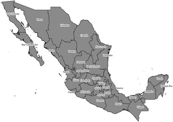
FIGURE 1 THE MEXICAN STATES
Source: Own elaboration, using QGIS software. Map taken from: www.diva-gis.org
2. METHODOLOGY AND SOURCES
The Instituto Nacional de Estadística y Geografía (INEGI), the Mexican official national institute of statistics, does not have any estimates of the states’ GDP for the years before 1970 (INEGI 1985). For previous years, scholars have commonly used the estimations made by Kirsten A. Appendini (Reference Appendini1978), either directly or as a basis for new estimations (Esquivel Reference Esquivel1999; Germán-Soto Reference Germán-Soto2005; Ruiz Reference Ruiz2006, Reference Ruiz2007, Reference Ruiz2010). Appendini estimated regional GDPs for 1900, 1940, 1950 and 1960 using a homogenous methodology (see Unikel et al. Reference Unikel, Ruiz-Chiapetto and Garza1978)Footnote 3 . The method used by Appendini (Reference Appendini1978) consists of disaggregating the national output of each sector across states according to the relative participation of each state in certain output indicators, measured at state level.
More recently, Ruiz (Reference Ruiz2007) offered an alternative estimation of regional per capita GDPs at state level for the years 1930, 1940, 1950, 1960 and 1965. This author uses the series provided by Appendini (Reference Appendini1978) as a basis for all his estimates, and applies a very similar estimation methodology (see Ruiz Reference Ruiz2006)Footnote 4 .
As previously mentioned, this study aims to estimate regional GDP per capita figures from 1895 to 1930Footnote 5 . As in previous research, for each sector, the national GDP across states is disaggregated on the basis of several indicators. This implies that, for each sector, the sum of all states’ GDPs is equal to the national GDP. As mentioned above, priority is given to direct production sources. Only in those sectors for which there is no direct information, such as industry for the early years and most services for the whole period, is the indirect methodology developed by Geary and Stark (Reference Geary and Stark2002) applied.
Geary and Stark’s methodology is an indirect estimation technique to distribute national GDP figures among regions, under the assumption of perfect factor mobility and well integrated national markets. This method uses information on relative wages and sectoral shares of employment. The authors assume that each region’s sectoral productivity is reflected in its sectoral wage, relative to the national sectoral wage. Thus, a region’s sectoral output is sector labour force multiplied by sector labour productivity. GDP in each region is the sum of its sector outputs (Geary and Stark Reference Geary and Stark2002, p. 921).
This methodology has been used in many recent works with a historical scope (Crafts Reference Crafts2005; Felice Reference Felice2009; Rosés et al. Reference Rosés, Martínez-Galarraga and Tirado2010; Henning et al. Reference Henning, Enflo and Andersson2011; Martínez-Galarraga Reference Martínez-Galarraga2012; Badia-Miró et al. Reference Badia-Miró, Guilera and Lains2012)Footnote 6 . Following Geary and Stark (Reference Geary and Stark2002, p. 933), regional GDP is defined as
 $$Y=\mathop{\sum}\limits_{}^i {Y_{i} } $$
where Y i is the state GDP, defined as
 $$Y_{i} =\mathop{\sum}\limits_{}^j {y_{{ij}} \,L_{{ij}} } $$
y ij and L ij being, respectively, the output per worker and the number of workers in state i and sector j. As we have no data for y ij this value is proxied by the product of the national sectoral output per worker (y j ) times the ratio between the state’s sectoral wage and the Mexican average wage for this sector (W ij /W j ), under the assumption that each state’s labour productivity in each sector is proportional to that state’s sectoral wage. Thus, regional GDP is given by
 $$Y_{i} =\mathop{\sum}\limits_{}^j {\left[ {y_{j} \,\beta _{j} \left( {{{W_{{ij}} } \over {W_{j} }}} \right)} \right]\,L_{{ij}} } $$
where y j is the national output per worker of sector j and β j is defined as a scalar, which preserves the relative state differences but scales the absolute levels so that the state totals for each sector add up to the known national total:
 $$\beta _{j} ={{Y_{j} } \over {\mathop{\sum}\nolimits_{}^i {\left[ {y_{i} \,\left( {{{W_{{ij}} } \over {W_{j} }}} \right)} \right]\,L_{{ij}} } }}$$
There is a potential problem involved with the application of this method to the Mexican case, which is associated with the Mexican labour market structure at the time. According to Kuntz:
[during the Porfiriato] although both population and the monetized sector of the economy increased, thousands of people still remained in their rural communities or haciendas as indentured labourers, and rarely participating in the market. […] In the South, masses of workers were incorporated into coffee and henequen plantations under labour relations that combined some degree of extra-economic coercion with low wage pay. However, it is not possible to estimate the number of workers involved
(Kuntz Reference Kuntz2010, p. 327, my translation).
This situation could distort the results due to the underestimation of labour productivity, which might introduce biases in the distribution of national GDP among regions. However, this problem seems to affect mostly the primary sector, which is precisely the sector for which direct output information is most abundant and, therefore, where it is not necessary to apply the Geary and Stark methodology. In the case of the secondary and tertiary sectors there is abundant evidence of labour market mobility across regions and sectors, responding to economic incentives such as higher relative wages (Kuntz and Speckman Reference Kuntz and Speckman2011, p. 517). For instance, Aurora Gómez-Galvarriato has found, in the case of the textile industry (the most developed one during the Porfiriato), that: «…In 1893-1896 there existed a strong relationship between these two variables [labour productivity and wages]. (…)» (Gómez-Galvarriato Reference Gómez-Galvarriato2002, p. 299). In other words, the Geary and Stark methodology is only applied to the industrial sector and some of the service sectors, which may be assumed to be less seriously affected by labour market rigidities. To prove the robustness of applying this methodology in the estimation, Figures 2 and 3 show the correlation between the states’ shares in the 1930 manufacturing output that result from applying both the direct production and Geary and Stark’s methodologiesFootnote 7 . As can be seen, the correlation between both values is fairly high, suggesting that the use of this methodology for previous years may provide likely results.

FIGURE 2 DISTRIBUTION OF THE MEXICAN MANUFACTURING GDP BY STATES IN 1930
Source: See text.

FIGURE 3 DISTRIBUTION OF THE MEXICAN MANUFACTURING GDP BY STATES IN 1930
Source: See text.
Another estimation problem is related with the changes in the Mexican administrative division. During the period under study (1895-1930), the current state of Quintana Roo (which was only established as an autonomous state in 1974) changed its status several times, being considered either as a federal territory or as a part of the Yucatán state. To allow comparability of the estimates over time, it was necessary therefore to include Quintana Roo within the state of Yucatán for the entire period, even in those cases for which data are available for Quintana Roo as an independent state. Furthermore, during this period, the Baja California peninsula (nowadays divided into two autonomous states: Baja California North and Baja California South) was a single federal territory. Therefore, for the period 1895-1930, the peninsula of Baja California is considered a single unit of analysis.
There are two main series of Mexican aggregate GDP for the period under consideration, which were estimated by Enrique Pérez (Reference Pérez1960) and Mario Gutiérrez Requenes (Reference Gutiérrez Requenes1969) and cover the years 1895-1959 and 1895-1967, respectively. Both estimations have been used repeatedly in other works, and the National Institute of Geography and Statistics (INEGI) reproduced Pérez’s estimation in the «Estadísticas Históricas de México» (2009). These, in turn, were used by Angus Maddison (Reference Maddison1992) and Barro and Ursúa (Reference Barro and Ursúa2008) in their databases. On the other hand, Leopoldo Solís used Gutiérrez Requenes’ series in his work «La realidad económica mexicana: retrovisión y perspectivas», which has been widely used by Mexican and international scholars (Solís Reference Solís1970), and the Bank of Mexico also included this series in its database.
As in the case of Appendini et al. (Reference Appendini, Murayama and Domínguez1972), Gutiérrez Requenes’ (Reference Gutiérrez Requenes1969) national GDP series are used for our estimates, for two main reasons. First, Gutiérrez Requenes (unlike Pérez), was explicit regarding both the methodology applied and the sources used for his aggregate GDP estimation. Second, Gutiérrez Requenes’ (Reference Gutiérrez Requenes1969) GDP is disaggregated into thirteen sectors (agriculture, livestock, forestry, fishing, mining, oil, manufacturing, construction, electric energy, transport, government, commerce and others), while Enrique Pérez’s GDP is only disaggregated in seven subsectors (agriculture, livestock, mining, oil, manufacturing, transport and other activities). Both reasons are important for this research since, whereas knowing the data and the method used by Gutiérrez Requenes to reconstruct the national GDP allows a more consistent estimation of regional figures, its more detailed disaggregation also allows a more precise distribution of national output. Nevertheless, it is important to stress that both series present very similar trends and fluctuations over the period analysed.
As previously mentioned, the different sectors of Gutiérrez Requenes’ national GDP database among states are distributed following different proceduresFootnote 8 . First, sectoral production was distributed directly, on the basis of output indicators, in the cases of the primary sector (which includes agriculture, livestock, forestry and fishing), mining, oil and commerce. By contrast, the secondary sector (i.e. manufacturing – with the exception of 1930 – construction and electric energy) and services, with the exception of commerce (i.e. transport, government and others), are obtained by using the Geary and Stark (Reference Geary and Stark2002) methodFootnote 9 .
For those sectors in which the estimates are based on production values and depending on the availability of data, information in current or in constant prices is used in each case. Thus, while in agriculture and livestock data in current prices are used for the entire period, in mining and forestry (with the exception of 1930) information is available in constant prices (gold pesos). The estimates of the commerce sector are also constructed using data in constant prices (with the exceptions of 1921 and 1930). When current prices are used, inflation differentials across states could affect the relative participation of each state in the indicator of dispersion. Unfortunately, there are no index prices at the state level for the entire period that would allow us to correct this issue. This potential distortion is not present when the estimates are based on data in constant (national) prices, or in the oil sector, in which units of production (barrels produced) are used. Finally, it is also absent from those sectors in which the estimates are based on Geary and Stark’s methodology (i.e. the secondary sector, with the exception of manufacturing in 1930, and the services sector, with the exception of commerce), although this is dependent on the assumption that differences in wage levels across states reflect productivity differentials. Therefore, it is fairly unlikely that inflation differentials across states change the global estimate’s results.
In the next lines the methodology and sources used for each year and each economic sector are described in detail.
2.1 Primary Sector: Agriculture
Agriculture is the sector for which quantitative information is most abundant during the period of analysis. For the years 1895, 1900 and 1910, the distribution of the national agriculture output among states is based on the production of twelve products: corn, bean, barley, wheat, sugar cane, cotton, henequen, coffee, tobacco, chickpeas, vanilla and rubberFootnote 10 . This sample includes those crops that were relatively important not only at the national level, but also at the state level. Thus, for instance, although henequen production only accounted for a low share of the national production, it was extremely concentrated in one state (Yucatán). According to the Estadísticas Económicas del Porfiriato: Fuerza de trabajo y actividad económica por sectores (1964), these products represented 81.5, 80.8 and 79.9 per cent of the total agricultural production in 1895, 1900 and 1910, respectively. The volume of production is taken from the Mexican Statistical Yearbooks published in those years, and prices come from the Estadísticas Económicas del Porfiriato (at current prices). The prices of corn, wheat and beans are available at state level. For the rest, prices are at national level.
For 1930, the national agricultural output is distributed according to the states’ total agriculture production value, taken from the First Census of Agriculture and Livestock of that year. Finally, in the case of 1920 the quantity and quality of the available official statistical data is much worse, due to the Civil War’s impact on public institutions during the 1910s and 1920s. Therefore, there are no available data at the state level for most crops, and only some scattered information on some products such as corn, wheat and bean. For this reason, the agriculture values of 1921 are obtained by doing a lineal interpolation of the share corresponding to each state in 1910 and 1930.
It was necessary to introduce some corrections to the raw data. In a few cases, state-level prices of certain crops (such as corn, wheat or bean) were extremely high, distorting the general estimation. In those cases, average prices of the Regional Division to which the state belongedFootnote 11 were taken. Thus, in 1895 and 1900, the prices of corn, wheat and bean in Chiapas and Oaxaca were replaced by the average prices of the South Pacific region, and, also in 1895, the price of corn in Veracruz was replaced by the average price of the Gulf of Mexico region. For 1910, the same correction had to be performed for the prices of corn in Sonora and Campeche, the price of wheat in Guerrero and Sonora, and the price of beans in Chiapas. Due to the absence of prices for Quintana Roo for 1910, the price in Yucatan was applied. Finally, the production data of coffee, vanilla and tobacco in Oaxaca for 1895 (which were surprisingly high) were replaced by the average of the 1894 and 1896 figures, except in the case of vanilla, in which the 1898 figure is used, due to the absence of information for the previous years. The final estimates of state agricultural output can be seen in Table A3.
Some particular states experienced a high variability in agricultural production during the period under study. This was largely related with significant changes in their production structure during the first globalisation. For instance, in Baja California the increase in cotton production provoked an upswing in the state’s participation in the national agriculture output from 1910 to 1921 and 1930. Yucatán’s share within the national agricultural output also varied widely, due to the fluctuations of henequen production, which was largely concentrated in this state.
2.2 Livestock
The only source that provides a complete livestock production database at the state level during the Porfiriato (1876-1910) is the 1902 Livestock Census, which is reproduced in the Estadísticas Económicas del Porfiriato…, and is the main source for our estimates for 1895, 1900 and 1910Footnote 12 . In other words, and due to the scarcity of information for the years 1895-1910, it had to be assumed that the distribution of livestock production across states remained constant throughout the period. It was only possible to take into account price differences among states, at least for some products. In our estimation the production of cattle, pork and milk are considered. Cattle and pork production is measured in kilograms (weighted in carcasses), and milk production in litres. According to the Estadísticas Económicas del Porfiriato… these products represented 89.49, 85.67 and 84.83 per cent in 1897, 1902 and 1907, respectively, of the total livestock production. Cattle and pork current prices are available at state level, but milk prices are only available at the national one.
The sources for 1921 and 1930 are the Statistical Yearbook of 1923-1924 and the First Census of Agriculture and Livestock (1930). For 1921 the total value of cattle, pork and goat (in current pesos) in 1924 is taken to distribute the national livestock GDP across statesFootnote 13 . In the case of 1930, poultry value is also considered. According to the mentioned sources, these products amounted to 79.5 and 83.3 per cent of total production in 1921 and 1930, respectively. Table A4 presents the new estimates of livestock production at state level for all benchmark years.
2.3 Forestry and Fishing
Information on forestry is also available in the Statistical Yearbooks for the years 1895 to 1910. For 1895, tanning bark – in kilograms – is the only possible proxy for production in this sector, and for 1900 and 1910 the production value (in gold pesos) of mahogany, cedar, mesquite, pine and oak is considered. These products represent 74 and 73 per cent of total forestry production in 1900 and 1907, respectively (Estadísticas Económicas del Porfiriato…). As in agriculture, no information is available for forestry around 1920, and the regional distribution of forestry production is assumed to be the same in 1921 and 1930. The source for the 1930 estimation is the First Census of Agriculture and Livestock (1930), which provides the Total Value of Forestry Production (in current pesos) for each state.
Fishing output at the national level is only available from 1921 onwards. This should not be a serious problem, since the share of this sector in the aggregate GDP is very low (0.04 per cent in 1921 and 0.09 per cent in 1930). As no statistical data are available for this sector at the regional level, the fishing production of 1921 and 1930 was distributed among the coastal states, weighted according to each state’s population. Table A5 presents the estimates for both forestry and fishing.
2.4 Mining and Oil
2.4.1 Mining
Mining GDP was distributed among states on the basis of information on the output distribution of both «mines in operation» and «metal production’ (excluding the iron and steel industry)Footnote 14 . The source for 1895, 1900 and 1910 is the Statistical Yearbook series, which gives production data («Metal Production Total Value» and «Mines Production Value») at state level in gold pesos Footnote 15 . The estimation of 1921 involves two steps. First, the share corresponding to «mines in operation» production is taken from the Mining Statistical Year Book of 1923 (Anuario de Estadística Minera, 1923). In this case, the «Production Value» in current pesos of gold, silver, lead and copper is added. These products account for around 85 per cent of the total production of «mines in operation» in 1923. Second, for «metal production», a lineal interpolation of the shares of the years 1910 and 1930Footnote 16 is carried out. For the 1930 estimation, the First and Second Industrial Censuses, carried out in 1930 and 1935, respectively, are used. Information on the output of the «mines in operation» is obtained from the 1930 Census, and data on «metal production» come from the 1935 Census («Total Value of production» in current pesos is used)Footnote 17 . Table A6 presents the estimation results.
In some cases, the state shares within the national mining output experienced wide fluctuations that can be explained easily. For instance, the high share of Chihuahua in 1930 is explained by the huge production of silver and lead around that year. That share was not exceptional since, in 1927, Chihuahua produced 32 per cent of the national mining production. On the other hand, the downtrend in Guanajuato in the 1920s and 1930s is explained by the deep mining crisis that took place in that state in those decades. Finally, the fluctuations in the Aguascalientes share can be explained by the arrival of the Guggenheim company at the end of the 19th century, which established one of the most modern mining plants in America at a time when capital was fairly unevenly distributed across Mexican states.
2.4.2 Oil
Oil production does not appear in national GDP until 1902 (with a very low participation in total production: 0.01 per cent); therefore, this sector is only considered from 1910 onwards. Oil production at state level, in barrel units, comes from Brown (Reference Brown1993), the Statistical Yearbook of 1923-1924 and the First Industrial Census (1930), for the years 1910, 1921 and 1930, respectively. Table A7 shows the oil production share at state level; as can be seen, oil production in those years was mostly located in Veracruz.
2.5 Secondary Sector
In the case of the secondary sector, the indirect Geary and Stark (Reference Geary and Stark2002) method was applied in order to distribute the national GDP across states, with the only exceptions of manufacturing and electric energy in 1930. As previously mentioned, this methodology requires, in addition to the national sectorial output, two main variables: labour force and wages, by economic sector and at the national and regional levelsFootnote 18 . In this regard, it was only possible to consider male workforce data, due to the serious biases involved in the available industrial female labour figuresFootnote 19 . This means, according to the Geary and Stark methodology, that the population share and the productivity of the female workforce in each state are assumed to be the same (relative to the national average) as that of the male workforceFootnote 20 .
2.6 Manufacturing
For 1895, 1900 and 1910, manufacturing labour force data are obtained from the First, Second, and Third Mexican Population Censuses published by Dirección General de Estadística, and wages come from Estadísticas Económicas del Porfiriato… (1964). Actually, for these years wages are only available for the following macro-regions, which include several states: North, Gulf of Mexico, North Pacific, South Pacific and CentreFootnote 21 . For the 1921 estimation, labour force comes from the Fifth Mexican Population Census and each state’s relative wage is obtained as a weighted average of the relative wages of 1910 and 1930 (the latter are taken from the First Industrial Census, 1930)Footnote 22 . Finally, the 1930 estimation is taken directly from the First Industrial Census (1930), which provides the total value of production and inputs. Table A8 shows the estimates for this sector.
2.7 Construction and Electricity
Construction and electricity sector estimates are obtained by applying the Geary and Stark methodology for all years, with the exception of the electricity sector in 1930, for which production data from the First Industrial Census are used. The male workforce is taken from the Population Censuses of 1895, 1900, 1910 and 1940Footnote 23 . For 1921, the same workforce structure across states as in 1910 is assumed (because the Population Census of 1920 does not provide disaggregated data of these sectors). On the other hand, wages in the construction and electricity sectors are assumed to be the same as in manufacturing. Table A9 shows both estimations.
2.8 Services: Government, Transport, Others
Government, transport and others services’ regional GDPs are also obtained by applying the Geary and Stark methodology. The male workforce for the three subsectors comes from the corresponding Population Censuses (1895, 1900, 1910, 1921 and 1930). In the case of government, the population employed in «public services» and «armed forces» for the years 1895, 1900 and 1910 is added, while for 1921 and 1930 «public administration» workers are added. Government wages at state level come from two sources: Estadísticas Económicas del Porfiriato… from 1895 to 1910 – for which a weighted average of «public services» and «armed forces» wages is estimated – and the Statistical Yearbooks of 1930 for wages in 1921 and 1930 – in these years, wages in the «executive power» sector are used.
For the transport sector data on the workforce in «communications and transports» are used, and the male workforce of «other services» is the sum of «professionals» and «other services» workers in 1895, 1900 and 1910, and the sum of «free professions» and «non-specific occupations» workers in 1921 and 1930. As no wage data are available for these subsectors, wages are assumed to be the same in all regions. This means assuming equal labour productivity in those sectors across all states. The estimation results for these three subsectors are presented in Table A10.
2.9 Commerce
In the case of commerce – the only service subsector for which a direct production indicator is available – a direct estimation is carried out on the basis of data on «declared sales» at state level. This information comes from the Fiscal Statistics Bulletins (1895, 1900 and 1910), and the Bulletins of National Statistics (1921 and 1930). The «declared sales» data is based on the stamp duty – which was a federal tax with the same specifications across all states. Due to the scarcity of information, the «declared sales» of 1918 and 1924 are used to estimate the 1921 and 1930 figures, respectively. The final results are shown in Table A11.
3. MEXICAN REGIONAL PER CAPITA GDPs, 1895-1930
3.1 The New Estimates: A Global Overview
Figure 4 shows the per capita GDP estimates of the Mexican regions between 1895 and 1930. These results are fairly consistent with the economic history literature and show that Mexican regional inequality was very high from the first stages of the process of national market integration. Regional disparities become even clearer when the states are grouped in macro-regions, showing the long-term differences between the north and the south of the country (see Table 1).
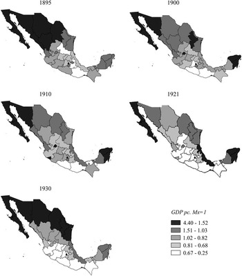
FIGURE 4 REGIONAL GDP PER CAPITA IN MEXICO 1895-1930 (MEXICO=1)
Note: The intervals displayed in the legend are obtained as follows: the relative values estimated for all years are put together and ranked from the highest to the lowest in order to construct one single vector. Finally, this vector was divided into five groups with the same number of observations. Source: See text.
TABLE 1 REGIONAL PER CAPITA GDP IN MEXICO, 1895-1930 (Mexico=1)

Source: See text.
In some regions, relative per capita GDP experienced wide fluctuations over time. This is the case, for instance, of Aguascalientes, which started with a GDP per capita of 1.06 in 1895 – always considering the national average as the unit of reference – increased to 2.65 in 1900, and ended with a GDP per capita of 0.88 in 1930. Although such processes will be analysed and explained in detail in further research, the relatively fast process of structural change in certain regions – such as the mining production areas – and some external shocks (such as international demand fluctuations or movements in the prices of some exportable agrarian and mining commodities) could largely explain these cases of high instability.
Moving to the sector level, Table 2 shows the spatial distribution of Mexican manufacturing GDP from 1895 to 1960. The spatial distribution of this sector has often been identified as one of the most important explanatory factors of the evolution of Mexican regional inequality, at least since the middle of the 20th century. The table shows that, while the centre region went through a process of de-industrialisation throughout the period, the north and the capital regions became more industrialised. Moreover, the coefficient of variation suggests that manufacturing spatial dispersion started to increase at least since the 1910s.
TABLE 2 SPATIAL DISTRIBUTION OF MEXICAN MANUFACTURING GROSS VALUE ADDED (percentage)

The regions are composed by the following states. Capital: Estado de México, Mexico City; North Gulf: Nuevo León, Tamaulipas; North: Chihuahua, Coahuila; North Pacific: Baja California Norte, Baja California Sur, Sonora, Sinaloa, Nayarit; Centre Gulf: Veracruz, Tabasco; Centre Pacific: Jalisco, Michoacán, Colima; Centre: Guanajuato, Querétaro, Hidalgo, Tlaxcala, Puebla, Morelos; Centre North: Aguascalientes, Durango, Zacatecas, San Luis Potosí; Peninsula: Yucatán, Quintana Roo, Campeche; South Pacific: Guerrero, Oaxaca, Chiapas. The coefficient of variation (CV) was obtained by considering the percentages at the state levels.
Source: From 1895 to 1930: own estimates; from 1940 to 1960: Ruiz (Reference Ruiz2014).
This would partially contradict some recent research, in which the process of concentration of industry in Mexico City has been assumed to have started with the ISI policies. Nevertheless, our new estimates suggest that this process of manufacturing concentration began well before the import-substituting industrialisation period (although it accelerated significantly after 1930).
3.2 Comparison With Previous Estimates
As previously mentioned, there are no previous regional GDP figures available for Mexico for the years 1895, 1910 and 1921. So far, the estimates by Appendini (1972) and Ruiz (Reference Ruiz2007) are the only Mexican regional per capita GDPs available for the years 1900 and 1930 (see section 2). Thus, it is only possible to carry out a comparison of our estimates for these 2 years. Table 3 compares our figures for 1900 with those of Appendini.
TABLE 3 COMPARISON OF 1900 REGIONAL GDP PER CAPITA (Mexico=1)

Source: See text.
Broadly speaking, the position and the values of each region are quite similar. Nevertheless, there are some remarkable differences in the cases of Baja California – in this case, the main difference is not the position but the GDP level – Aguascalientes, Morelos, Jalisco, Tlaxcala, San Luis Potosí and the state of Mexico. There are other less significant differences, such as the cases of Chihuahua, Sinaloa, Tamaulipas, Tlaxcala and Guanajuato. In order to identify the reasons for the main differences, Table 4 compares Appendini’s estimates with our figures at sectoral levelFootnote 24 .
TABLE 4 PERCENTAGE OF SECTORAL GDP, 1900 (COMPARISON BETWEEN APPENDINI’S ESTIMATION AND MY OWN FIGURES)

Source: See text.
When GDP figures are disaggregated among sectors, the differences between both estimations increase significantly. As can be observed in the table, the main differences arise in both mining and manufacturing. The differences in the mining sector result from the fact that, in the new estimation, the production values of «mines in operation» and «metal production» are considered from the Statistical Yearbooks, whereas Appendini’s estimates only take into account the distribution of the former, from the same source.
In the case of manufacturing, differences can be explained because, whereas for our estimate the Geary and Stark (Reference Geary and Stark2002) method was applied, Appendini (1972) used the industrial production data taken from the Industrial Census of 1902 (DGE 1903). The main problem of using the Industrial Census is that it seems to be highly biased due to the exclusion of the traditional manufacturing production, and the absence of many industrial establishments. Therefore, the representativeness of this census is rather low and uneven across states, causing high distortions in the estimation. As is pointed out in the introductory part of the census:
The industry in Mexico is very widespread; there is a great amount of self-employed persons working at a very small scale, and this has undoubtedly caused that it was not possible to obtain enough data, and that countless cases of concealing happened, so only limited data supplied by some important industrial establishments were available. (…) For these reasons, it will be seen that only the data that have been possible to collect are published, and surely there are many more industrial establishments than the ones enumerated in this work… .
(DGE 1903, p. ii, my translation)
This problem also shows up when observing the industrial workforce registered in the Industrial Census, which amounts to just 24 per cent of the total industrial workforce recorded in the Population Census of 1900. This introduces biases at state level. For instance, the manufacturing workforce listed in the 1902 Industrial Census for the states of Guanajuato and Nayarit correspond to 6.2 and 92.45 per cent, respectively, of that registered in the Population Census of 1900.
By contrast, differences in the share of services between the two estimates are minor. This is because the weight of commerce within the services sector is very high (around 51 per cent) and, for this subsector, both sets of figures have used the same proxy (declared sales) to distribute the national commerce output across statesFootnote 25 .
Finally, a comparison between our estimates and the 1930 figures proposed by Ruiz (Reference Ruiz2007, p. xxix) is shown in Table 5. Once again, the differences are minor when total state values are considered. Ruiz’s data allow comparisons of the two estimates for the industrial sector (Table 6). As shown in the table, while manufacturing estimates are fairly close, the construction subsector presents wider differences. This could be explained because Ruiz assumed equal productivity across states, while we applied the Geary and Stark method (see previous section).
TABLE 5 GDP PER CAPITA, 1930 (COMPARISON BETWEEN RUIZ’S FIGURES AND AGUILAR-RETURETA (highest value=100))

The comparison is presented in this form because there is no other figure available in Ruiz (Reference Ruiz2007).
Source: See text.
TABLE 6 PERCENTAGE OF SECTORAL GDP, 1930 (COMPARISON BETWEEN RUIZ’S FIGURES AND AGUILAR-RETURETA)

Mexico City’s high share in construction (48%) in 1930 would be consistent with this region having 83.2% of the total construction output in 1960, according to the VII Industrial Census (1960).
Source: See text.
4. THE REGIONAL GDP PER CAPITA IN MEXICO. A LONG-TERM PICTURE (1895-2010)
To link these new regional per capita GDP estimates for the years 1895-1930 with those available for 1940-2010, German-Soto’s (Reference Germán-Soto2005) GDP figures for 1940-2000, and the INEGI estimates for 2010 are used as well as the corresponding National Population Censuses to express GDP in per capita termsFootnote 26 . In order to account for the extreme spatial concentration of oil production, the states’ GDP for 1940-2010 excluding oil production was also estimated. From 1940 to 1960, the percentage of each state’s oil production is taken from Ruiz (Reference Ruiz2007) and, for 1970-2010, it is available in INEGI (1985, 2002, 2014). These figures can be linked to our own estimates without oil production for the period before 1940, obtaining as a result two state GDP databases, with and without the oil sector, for the whole period 1895-2010 (Table 7).
TABLE 7 REGIONAL PER CAPITA GDP IN MEXICO: 1900, 1930, 1950, 1980 AND 2010 (Mexico=1)

Source: See text.
1 Oil production excluded.
Table 7 shows the high persistence of the states ranked in the extreme positions, especially in the case of the poorest ones which, in turn, are concentrated in the centre and south of the country. In contrast, Mexico City and the northern regions have always remained in the top places. Although this pattern will be explained in detail in forthcoming research, this persistence could be mainly explained by the economic specialisation of each state, with the north region and Mexico City having an economic structure with a relatively higher productivity due to a higher presence of manufacturing activity (see Table 2).
The rank ratio displayed at the bottom of Table 7 (which indicates the ratio between the per capita GDPs of the richest and poorest states), reached its maximum value at the end of the agro-export model (1930), when the richest state (Baja California) had a GDP per capita (with and without oil production) that was ca. 15.7 times as large as the poorest state’s per capita GDP in the same year (Guerrero). The ratio substantially decreased thereafter, reaching its minimum level at the end of the ISI period, in 1980.
In order to provide a more complete perspective of regional income inequality trends in the long run, Figure 5 depicts the standard deviation (with and without oil production) and the Theil index (without oil production) of the Mexican states’ GDP per capita Footnote 27 . Both indexes have often been used to test σ convergenceFootnote 28 . As can be seen in the graph, both indicators follow a fairly similar N-shape trend over the period, in which trend changes generally coincide with changes in economic model. To start with, during the agro-export model, dispersion increased, reaching its maximum level during the 1930s. Thereafter, as has been shown by previous literature, it gradually declined during the ISI period, from 1940 to 1980 (Esquivel Reference Esquivel1999; Ruiz Reference Ruiz2010). However, the trend was reversed again from 1980 onwards, when Mexico started a process of increasing openness (Sánchez-Reaza and Rodríguez-Pose Reference Sánchez-Reaza and Rodríguez-Pose2002; Chiquiar Reference Chiquiar2005). Income dispersion (excluding oil production) would have stopped its growth in the first decade of the 21th century, although we still do not have a long enough perspective to know whether this change will be sustainedFootnote 29 .

FIGURE 5 STANDARD DEVIATION AND THEIL INDEX OF MEXICAN STATES GDP PER CAPITA, 1895-2010
The long-term trend of Mexican regional income inequality does not seem very different from those observed in Britain (Crafts and Mulatu Reference Crafts and Mulatu2005), France (Combes et al. Reference Combes, Lafourcade, Thisse and Toutain2011), Portugal (Badia-Miró et al. 2012) or Spain (Rosés et al. Reference Rosés, Martínez-Galarraga and Tirado2010). In contrast, the Mexican experience has been rather different from the Chilean experience (the other Latin American economy for which similar data are available; Badia-Miró Reference Badia-Miró2014). In Chile, there has been a continuous process of regional convergence from the late 19th century to the present. The reasons behind the difference between these two economies will be the subject of future research.
In order to complement the σ-convergence analysis, Figure 6 tests unconditional β convergence for both the entire period (1895-2010) and the time span of our new estimates (1895-1930)Footnote 30 . The results are very different. Figure 6A shows clear evidence of unconditional β convergence across Mexican states in the long term. By contrast, in Figure 6B the β-convergence hypothesis must be rejected for the period 1895-1930, given the lack of correlation between initial per capita GDP and the growth rate. Future research will also focus on the forces behind convergence (or its absence) in different periods.

FIGURE 6 (A) MEXICAN UNCONDITIONAL β CONVERGENCE AT THE STATE LEVEL, 1895-2010. (B) MEXICAN UNCONDITIONAL β CONVERGENCE AT THE STATE LEVEL, 1895-1930
5. CONCLUSIONS
So far, the only available estimates of Mexican regional GDPs for the period before 1940 were those of Appendini (1972) for 1900 and Ruiz (Reference Ruiz2007) for 1930. This paper has presented the methodology, sources and results of a new regional GDP per capita estimation in Mexico for the benchmark years 1895, 1900, 1910, 1921 and 1930. The new evidence suggests that the regional disparities between the north and south of the country can be traced back at least to the early stages of the integration of national markets. These disparities widened between 1895 and 1930, due to a large extent to the progress in the industrialisation of the capital and northern regions, and the de-industrialisation of the centre regions. As a result, it was during the 1930s, at the end of the export-led growth episode of Mexican history, when the country’s regional inequality reached the maximum level. Thereafter, inequality started a sustained decrease that coincided with the ISI period, until a new increase in inequality started in the 1980s, largely associated with increasing economic openness.
Future research will focus on the patterns and causes of spatial inequalities in Mexico over the long term. Even though regional inequality has been well studied, scholars have focused on recent periods (and especially on the transition from a relatively closed economic model to an open one, between 1980 and the present). These new estimates will make it possible to study the inverse process that took place since the interwar period, that is, when the economy changed from a relatively open model to a relatively closed one. Moreover, these analyses will provide us with the necessary tools to answer some relevant questions, such as: What are the causes behind the evolution of regional income inequality in Mexico during the period of national market integration and early industrialisation? Do the theoretical assumptions of the New Economic Geography apply for the Mexican case in the long term? Are the mechanisms behind Williamson’s inverted-U hypothesis confirmed for a non-core economy? The answers to these questions may contribute to the international literature on historical regional inequality, providing evidence, unlike most available literature, on an economy outside the Western core.
Supplementary Material
To view supplementary material for this article, please visit http://dx.doi.org/10.1017/S0212610915000117


