
Introduction
Within the diverse literature on alternative food systems, there is a history of associating ‘localness’ with sustainability. This connection has been traced to the writings of Wendell Berry, Jim Hightower and Frances Moore Lappé from the 1970s, which articulated a vision for local, sustainable and just food systemsReference Feenstra1. Geographic proximity has been related to sustainability for a variety of reasons, encompassing the ecological, economic and social dimensions of the food system. For example, in local food systems where producers and consumers are in closer physical proximity, local food is presumed to travel shorter distances and consequently reduce the amount of energy usedReference Kloppenburg, Hendrickson and Stevenson2–Reference Gussow and Clancy5 and greenhouse gas emissions releasedReference Pirog, Van Pelt, Enshayan and Cook6 in the transport of foods. Similarly, local food is presumed to be marketed either directly to consumers or through shorter supply chains, enabling farmers to capture a greater share of the food dollar and thereby improve the economic viability of farms and rural communitiesReference Halweil3, Reference Gussow4, Reference Lyson and Green7, Reference Magdoff8. Moreover, the closer relationship between farmers and the general public is purported to increase awareness of issues related to the food systemReference Gussow4, Reference Magdoff8. Taken together, these reasons make a case for why local foods or food system ‘localization’ should be a vital component of a transition to a more sustainable food system.
The veracity of these claims has become a matter of debate in both the academic literature and the popular press. Major mainstream periodicals have recently featured articles that discuss merits of purchasing local food with regard to reducing environmental impact9, Reference Cloud10. Similarly, articles in academic journals have questioned the assumption that local food systems are intrinsically more just or sustainable than the conventional food systemReference Bellows and Hamm11–Reference Born and Purcell13. In response to growing interest in the topic, a group of researchers from the UK reviewed the literature to test the claim that local food actually reduces emissionsReference Edwards-Jones, Milá i Canals, Hounsome, Truniger, Koerber, Hounsome, Cross, York, Hospido, Plassman, Harris, Edwards, Day, Tomos, Cowell and Jones14. They concluded that a sufficient body of analysis does not exist to substantiate or refute the claims. The debate remains unresolved. However, the pressing concerns of climate change, rising energy prices and the longevity of fossil fuel supplies suggest that the degree to which societies can continue to depend on food transported long distances is a relevant questionReference Peters, Bills, Wilkins and Fick15.
The world is increasingly urban. It is projected that in 2008 more than half of all people will live in cities16. In this context, if ‘localizing’ the food system is an important principle of or strategy for improving sustainability, a fundamental question to ask is, ‘To what degree can food be produced locally?’ Moreover, should the meaning of ‘local’ be context specific? While the term ‘local’ lacks consistent definition, various attempts have been made to estimate the capacity for circumscribed areas (individual states within the USA or, in the case of the UK, an entire country) to meet their internal food needs. Some analyses examine the potential for current production to satisfy current consumptionReference Messing17–Reference Peters, Bills, Wilkins and Smith22. Others estimate how agricultural production or diets could change to enable a larger share of food to be produced locallyReference Stephens, Fleming, Gacoin and Bravo-Ureta18, Reference Peters, Wilkins and Fick23. However, they all examine their respective study regions in the aggregate. In contrast, a geospatial framework may allow one to investigate the capacity to produce food locally with greater geographic precision.
To this end, the concept of a ‘foodshed’ offers a possible framework for such analysis. In its original meaning, ‘foodsheds’ define the barriers that guide the flow of food from the producer to the consumerReference Hedden24, though the term has also been used to describe a food system that connects local producers and consumersReference Kloppenburg, Hendrickson and Stevenson2, Reference Halweil3, Reference Pretty25, Reference Feagan26. For the purposes of this paper, a potential local foodshed is the land that could provide some portion of a population center's food needs within the bounds of a relatively circumscribed geographic area. This concept provides a framework for analyzing the capacity to produce food locally at the scale of an indi-vidual city. However, no standard methods exist for analyzing foodsheds. Thus, the principal goal of this research was to develop a spatial model for mapping potential, local foodsheds.
To achieve this goal, the model uses a combination of geographic information system (GIS) and optimization techniques to analyze the capacity of New York State (NYS) population centers to meet their food needs within the state. The model estimates the distance within which food could potentially be supplied and, since previous research has shown that NYS cannot supply all of its food needsReference Peters, Wilkins and Fick23, the share of total food needs that could be met from in-state production. Moreover, the model enables the production of foodshed maps as a tool for visualizing the geographic extent of a food supply. As home to the largest city in the nation [(New York City (NYC)], the largest protected natural area in the 48 conterminous USA states (Adirondack Park27), and a multi-billion dollar agriculture industry, NYS makes for an interesting test case.
Methods
We developed a hybrid spatial-optimization model to map potential local foodsheds and to evaluate the capacity for NYS population centers to supply their food needs within the state's boundaries. The model characterized the food production potential of the state's land and the food needs of its population centers within a GIS. The GIS provided input for an optimization model that allocated NYS food production capacity to meet the food needs of NYS population centers in the minimum possible distance. The details of each step are outlined in the subsequent sections.
Outline of model design
A broad range of data were processed to create a GIS that produced input data for the optimization model used to map foodsheds (Fig. 1). Soil and land cover data provided estimates of the relative productivity of soils and the location of agricultural land in NYS. Urban area (UA) delineations and population data were used to determine the location of population centers and the numbers of people who reside in or near them. Data from prior research on the land requirements of the human dietReference Peters, Wilkins and Fick23 were used to derive estimates of per capita food need and average NYS food yields.

Figure 1. Simplified data flow diagram for the spatial model used to map potential local foodsheds.
The GIS integrated these data to produce input for the optimization model. Estimates of food production potential were calculated for each food-producing unit or production zone. Estimates of food needs were calculated for each population center. The GIS also calculated distances between all production zones and population centers. The resulting data matrices were incorporated into an optimization model that allocated available production to meet the needs of population centers such that the distance food traveled was minimized. Output from the model was used to map and characterize potential foodsheds. All mapping and geospatial operations were performed using ArcGIS 9.1 and Manifold® System 6.5.
A new unit for representing food in the aggregate
For this analysis, a unit is needed that can be used to measure both food need and food production. To this end, this study introduces a new unit for discussing food in the aggregate: the Human Nutritional Equivalent (HNE). An HNE is a basket of food that contains representatives from all food groups combined in the proper proportions to constitute a complete diet for one person for 1 year.
The USDA Economic Research Service (ERS) set a precedent for examining the adequacy of the USA agricultural production through the lens of a complete diet in the late 1990s. Rates of diet-related chronic disease and obesity motivated ERS to examine the relationships between American dietary habits and the food systemReference Kennedy, Blaylock, Kuhn and Frazao28. Researchers examined the adequacy of the USA food supply in light of the USDA Food Guide Pyramid (FGP) recommendationsReference Kantor and Frazao29 and estimated the changes in USA agriculture that would be required to enable all Americans to follow these recommendationsReference Young, Kantor and Frazao30. This approach offers a framework for assessing the adequacy of agricultural production in a broader context than simply measuring caloriesReference Peters, Fick and Wilkins31.
The concept of an HNE stems from this work. In theory, an HNE should represent a diet containing foods in adequate quantities and varieties to meet human nutritional requirements. Because of differences in food preferences or cultural values, diets can differ substantially in terms of specific foods included or excluded and can range from strict vegetarian to meat-centric. Thus, an HNE can reflect both dietary recommendations and food consumption preferences. As a result, the HNE is a valuable concept for comparing different strategies for meeting a population's food needs that are nutritionally comparable but may have very different land, or other resource, requirements. Such a measure could be valuable for multiple contexts, from farmland preservation to food security to the growing food versus fuel debate.
Diet and land requirements sub-model
Data from a sub-model were used to determine the composition of an HNE and the average yield of HNEs on NYS agricultural land. The sub-model was the product of previous research that calculated the area of land required to produce the annual food needs of the average person on NYS agricultural land according to a variety of diet scenariosReference Peters, Wilkins and Fick23. The design of the sub-model has been described in detail in this earlier work, but its basic methodology is reviewed here in brief.
The USDA FGP was the starting point for the 42 diet treatments embedded in the sub-model. The diet treatments varied in terms of the quantity of meat and fat they contained, but all diets were balanced to provide 2300 kcal per day, an amount adequate to meet the caloric requirements of the average New Yorker. Diets were constituted of representative food commodities from each food group, but, with the exception of sugar beet, included only commodities that are produced in NYS. Per capita intake of each food commodity in each diet treatment was estimated based collectively on the quantities of meat and fat in the treatment, the food group recommendations of the FGP, the serving size of the commodity and the relative preferences for that commodity from national food consumption survey data. Total edible food need was derived by inflating estimated intake to allow for the percentage of edible food in the food system that spoils or is otherwise wasted between the farm gate and the consumer.
To determine the land requirements for each food commodity, the estimates of food need were converted into quantities of agricultural commodities (crops and livestock) by using conversion factors to account for the removal of inedible portions and transformations that occur in food processing. Next, estimates of the quantity of livestock needed were used to derive the amount of feed crops necessary to supply the food coming from livestock. Finally, the quantities of feed and food crops were divided by average NYS crop yields to determine the average land requirements of the diet.
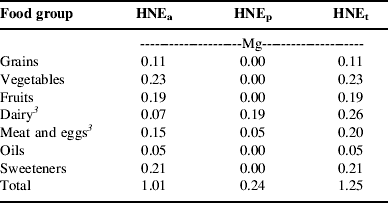
For the sake of this research, one diet was selected, from the many available in the sub-model, to represent food need. This diet meets USDA guidelines for all food groups, and, like the typical American diet, relies on meat and eggs, rather than pulses, as the major protein source. The composition of this diet is outlined in Table 1 that reports the quantity of food from each food group that would be required to feed the average person for 1 year according to the diet assumptions inherent in the model. The quantities are expressed in terms of the farm weight of agricultural commodities required to provide the food consumed in the diet.
Table 1. Constituents of a HNEFootnote 1 for the diet used in the foodshed model, expressed in farm weight of foodFootnote 2 and partitioned into HNEs derived from annual and high-value crops (HNEa), perennial forage crops (HNEp) and all crops (HNEt).

1 An HNE is the amount of food needed to provide one person a complete diet that meets all nutritional requirements for 1 year. See text for more details.
2 Farm weight of food is the quantity of agricultural commodities (i.e. wheat, fluid milk, live animals, etc.) required to produce the foods included in the diet. This weight includes nonedibsle portions that are removed in processing.
3 The dietary contribution of dairy and meat is divided between HNEa and HNEp based on the proportion of energy in the livestock rations that comes from annual crops (HNEa) or perennial forages (HNEp). Published estimates of total digestible nutrients (TDN) were used to measure the available energy in the feed crops. In the case of the meat and eggs food group, perennial crops only contribute to the production of beef, the only ruminant meat included in the diets.
Since not all land resources are equally suited to tillage and annual crop production, dietary requirements are partitioned into two categories: the quantity derived from annual and high-value crops (HNEa) and the quantity derived from perennial forages (HNEp). The sum of these two categories equals the total quantity of food (HNEt). The HNEa category aggregates grains, pulses, vegetables, fruits, oils, sweeteners and grain-based livestock. The HNEp category contains meat and milk from ruminant animals. Based on the diet shown in Table 1, an average person requires 1.25 Mg of HNEt annually, 81% of which come from HNEa and 19% of which comes from HNEp. Although individual food groups are shown in Table 1, the model only differentiates between these two categories of foods, HNEa and HNEp.
Estimating potential food production
The productive potential of NYS soils was determined using two sources of soils data. Spatial data on the distribution of soils were obtained from the State Soil Geographic (STATSGO) database32. Information on expected yields and recommended crop rotations for individual soils were obtained from the Master Soils List (MSL), a resource maintained by the Department of Crop and Soil Sciences at Cornell University and published annually by the NYS Department of Agriculture and Markets33. The integration of these two data sets is described below.
Data from STATSGO represent soils in a generalized manner appropriate for statewide and regional analyses34. Each STATSGO map unit contains multiple soil types, called components, each of which corresponds to a soil mapping unit from the county-level Soil Survey Geographic (SSURGO) database34. The MSL database provides information for all NYS soils, including all the mapping units in the SSURGO database. Thus, the data were integrated by matching each soil component in STATSGO to its corresponding soil in the MSL (for complete details, see Appendix 1 of PetersReference Peters35).
Once the two databases were joined together, the expected yields and recommended rotations were calculated for each STATSGO map unit. In all cases, the value assigned to the map unit was the average for all soil components in the map unit which had agricultural potential (i.e. nonzero yields), weighted based on the percentage that each component contributed to the total map unit area (see PetersReference Peters35 for more details). Together, these data provided estimates of the spatial variability in expected yield of two indicator crops, corn (Zea mays) silage and hay (multiple species). Corn silage was used to indicate the productive potential for annual and high-value crops (HNEa), and hay indicated the potential for perennial forage crops (HNEp). In addition, these data provided estimates of the maximum number of years (out of ten) that a piece of land should be planted to corn silage, in a corn silage–hay crop rotation, without causing soil erosion that exceeds the tolerable limit defined by the USDA Natural Resource Conservation Service. These recommended rotations were used to estimate the proper proportion of annual to perennial crops in the model, in other words the proportion of land that could be devoted to producing HNEa versus HNEp.
The location of agricultural land in NYS was determined using the most recent land cover data available at the time the study was conducted, the 1992 National Land Cover Dataset (NLCD)36. The NLCD data were processed to reduce inherent error as recommended by the US Geological Survey37. This involved using the data at the most general level of land cover classification (agriculture, barren, forest, urban, water and wetland) and performing some spatial aggregation (see Appendix 3 of PetersReference Peters35 for details). Next, the land cover data were intersected with soils data to create spatial layers that showed the location of agricultural land cover along with expected crop yields and recommended rotations of the underlying soils.
The combined soil and land cover data displayed potential productivity at a very fine resolution; each pixel represented a 30 m by 30 m land area. A pixel could not be considered as an independent production unit for two major reasons. First, this would create a problem with more vari-ables than could be handled in the optimization software. Secondly, such small units would not be managed inde-pendently for food production; they would be parts of larger fields. Thus, a set of data was created that represented the land area of NYS in 5 km by 5 km grid cells called production zones. For the sake of the model, each of these zones was a potential food-producing unit. The relative productive potential and land management limitations of each zone were estimated based on a spatial overlay of the production zone boundaries with the layers of combined soils and land cover data. Data from this overlay were used to derive food production potential (Eqn 1):
The production potential (P) of a given food category (i) for each production zone (j) was the product of the area in agricultural land cover (A), the expected yield (E) of the indicator crop, the recommended proportion of time (R) that the land can be devoted to the indicator crop and the average yield (Y) of the given food type in NYS, divided by the land area weighted average expected yield (Ē) of the indicator crop across NYS. The terms A, E, R and Ē were all calculated from the spatial data layers. The term Y was derived from the land requirements of diet sub-model and is expressed in Mg HNE per unit area.
Estimating food needs of population centers
By definition, a foodshed is the area of land from which a population center derives its food supply. The US Census Bureau's Urbanized Areas and Urban Clusters (UAUC) data38 were used to identify the locations of population centers. These data delineate clusters of contiguous, highly developed land throughout the USA, and thus represent population centers as discrete geographic entities. One hundred and thirty-two of these entities exist in NYS.
For modeling purposes, it was assumed that rural NYS residents would obtain their food from a population center. Thus, a method was devised to assign each member of the rural population to a nearby urbanized area (UA) or urban cluster (UC). According to the US Census Bureau39, the UAUC boundaries were created by aggregating smaller geographic entities, called census block groups, which exceed a threshold population density. Therefore, we estimated the number of people associated with a given population center using a GIS procedure that allocated the population of every NYS census block group40 to the nearest UA or UC. The food consumption capacity (C) of each population center (k) for a given food category (i) was equal to the number of people (N) residing in or near the population center multiplied by the weight (W) of food needed by the average person as indicated by the diet and land-use sub-model (Eqn 2):
Distance between production zones and population centers
The distance between production zones and population centers was estimated based on the distance from the geographic center of each production zone to the geographic center of each population center. The distances used in the model are Euclidian (as the crow flies), not distances along transportation networks.
Optimization: allocating the available production potential
The optimization problem solved in the foodshed model is an adaptation of the classic transportation problem in which the goal is to minimize the cost of transporting goods from multiple suppliers to multiple clients. Such an approach has been used by regional planners to estimate theoretical minimum commuting distances based on the locations of housing and workplacesReference Horner and Murray41. In this application of the foodshed model, the total population in the region of analysis was greater than the available land resources could support. Thus, the model allocated all available land while minimizing the distance food traveled. Were land in surplus, the model would seek to feed all people in the shortest total distance.
The optimization problem was set up as a matrix of producers and consumers in which each production zone is a potential supplier of food, both HNEa and HNEp, to each population center. The optimization software solved for the matrix of values that minimized the total food distance traveled throughout the study area. Total food distance (Eqn 3) was defined as the sum of the products of the quantity of food (F) from each category (i) allocated from each production zone (j) to each population center (k) and the distance (D) between the production zones and population centers. The value reached by the model was a global minimum for the entire state, but not necessarily the minimum for an individual population center since the most efficient allocation for the whole state might require that land near one population center be assigned to a more distant population center:
This optimization problem was subject to two categories of constraints. Since the study area contains more people than it can feed, the first set of constraints (Eqn 4a) required that the quantity of food (F) supplied to each population center (k) be less than or equal to the need (C) of the population center for a given type of food (i). These constraints prevent any population center from receiving more food than it needs, while allowing the model to leave the needs of some population centers unsatisfied. The second set of constraints (Eqn 4b) required that the quantity of food (F) supplied by each production zone (j) be equal to that zone's potential (P) for producing a given type of food (i). These constraints force the model to allocate all the food production potential available, and thus prevent the model from minimizing distance by allocating no food. The production potential of each production zone and the food needs of each population center were obtained using the equations described in earlier sections (Eqns 1 and 2, respectively).
Optimization was performed using the Premium Solver Platform™ v6.5 and the Extended Large-Scale LP Solver Engine v6.5 from Frontline Systems42, 43. These programs are upgrades of the basic solver in Microsoft Excel® and are accessed through the solver dialogue box in Excel®44, 45. Note that because this software operates within an Excel® worksheet, the organization of optimization problems is limited by the maximum numbers of rows (65,536) and columns (256) allowed by Excel®. Two columns were needed to represent each population center–food type combination (one to represent HNEa and another for HNEp), and several columns were used for problem setup. As a result, only 125 of the 132 NYS population centers could be accommodated by the model. Since the seven smallest NYS population centers contained only 36,737 people (just 0.2% of the total state population), they were simply excluded from the analysis. For a detailed description of the setup of the optimization problem, see the Appendix.
Results
Geography of food production potential
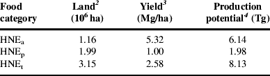
NYS has 3.15 million ha of agricultural land cover (Table 2). Because much of this resource has soils that are prone to erosion, nearly two-thirds of the land must be devoted to perennial forage crops, leaving slightly more than one-third for annual and high-value crop production. Yields of food, on a weight basis, are five times greater on land used for HNEa than HNEp. As a result, the foodshed model estimates that NYS agricultural land could produce 6.14 Tg of HNEa and 1.98 Tg of HNEp, given the dietary assumptions inherent in the model.
Table 2. Agricultural land area, average yields and total food production potential in NYS for each category of HNEFootnote 1.

1 An HNE is the amount of food needed to provide one person a complete diet that meets all nutritional requirements for 1 year. The diet is partitioned into food derived from annual and high-value crops (HNEa) and food derived from perennial forages (HNEp). Values are also shown for the total diet (HNEt). See text for more details.
2 Area of land available based on 1992 land cover data for NYS and recommended crop rotations for NYS soils. Despite the age of the land cover data, the total extent of agricultural land cover does not appear to have changed much since 1992. The 2003 National Resources Inventory reports that NYS has 3.24 million ha of cropland, pasture land and cropland reserve46. However, because of differences in methodology and definition, the total area of agricultural land cover in NYS is substantially larger than the areas of cropland and permanent pasture reported in either the NYS annual agricultural bulletins or the 5-year Census of Agriculture. For example, recent editions of the NYS annual bulletin on agricultural statistics and the Census of Agriculture reported, respectively, that the total area in cropland and permanent pasture on farms in NYS was 2.21million ha and 2.18 million ha (authors' calculations from New York Agricultural Statistics Service47 and USDA National Agricultural Statistics Service48 data).
3 Average yield for all production zones in the foodshed model.
4 May not exactly equal the product of land and yield due to rounding error.
This production potential exists throughout NYS, but it is not evenly distributed (Fig. 2). As the maps indicate, the areas with relatively greater potential to produce HNEa and HNEp (shown in darker shades) are concentrated in the western part of the State, where soils are generally well-suited to modern agriculture and large areas are used for agricultural purposes. In contrast, the eastern portion has large areas with low or no production potential (lighter shades and unshaded areas). These low-potential areas are generally either rural areas with poor soils and mostly forested cover (most notably, the Catskill and Adirondack mountains) or predominantly UAs that contain little agricultural land.

Figure 2. Maps of food production potential in NYS measured in mass of HNE. (a) Foods derived from annual and horticultural crops (HNEa). (b) Foods derived from perennial forages (HNEp).
Geography of food need
The residents of NYS are dispersed throughout a mixture of rural and urban places, but they are not evenly distributed. Of the 125 population centers considered in the model, 63% of the state's almost 19 million people reside in or near just one population center, the greater NYC area (Table 3). An additional 23% of the population resides in or near the 15 urbanized areas outside NYC, and the remaining 14% live in and around the state's more than 100 UCs. However, while NYC contains the large majority of the total and urban populations, most of the state's rural population live nearest to a UC or smaller urbanized area.
Table 3. Urban, rural and total populations of each category of NYS population center.
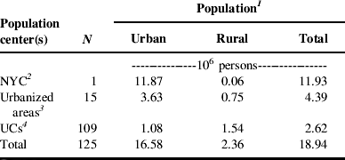
1 For modeling purposes, the total population within the foodshed of a population center includes nearby rural residents (see Methods section for details). Urban populations reside within the UAs or UCs that constitute the core of a population center, and rural populations reside outside these entities. Estimates of the urban population for individual UAs and UCs were obtained from the US Census Bureau49. Estimates of the rural population are the difference between the total population allocated to the population center and the estimate of urban population from the US Census Bureau.
2 The name ‘New York City’ is familiar to a wide audience and thus is used here to refer to the NYS portion of what the US Census Bureau defines as the ‘New York-Newark’ urbanized area. The population values shown include only the NYS residents.
3 Excludes NYC.
4 Excludes the seven smallest UCs in NYS. These population centers were omitted from the analysis for reasons discussed in the Methods section.
The individual population centers included in the model range in size from a few thousand people to more than 10 million (Fig. 3). While these population centers are distributed throughout the state, the population is heavily concentrated in the southeast corner, where NYC is located. Since per capita food need was assumed to be identical for all population centers, total food needs were distributed identically to population.

Figure 3. Locations and relative sizes of the population centers in NYS.
Allocating production potential to meet need: mapping foodsheds
Overall, the model shows that the capacity of NYS to produce food is insufficient to meet the total food needs. The population centers in the model required 23.6 Tg of HNEt, whereas the production potential of NYS agricultural land could only provide 8.1 Tg of HNEt or about 34% of the total food needs (Table 4). This capacity to meet food needs varied by food type. The NYS land base was better able to meet the needs of foods derived from perennial forages than those derived from annual and high-value crops, providing 44% of HNEp but just 32% of HNEa.
Table 4. Quantities of foodFootnote 1 allocated to each category of NYS population center relative to food needs.

1 Quantities of food are expressed in weight of HNEs. An HNE is the amount of food needed to provide one person a complete diet that meets all nutritional requirements for 1 year. The diet is partitioned into food derived from annual and high-value crops (HNEa) and food derived from perennial forages (HNEp). Values are also shown for the total diet (HNEt). See text for more details.
2 Totals may not add due to rounding error.
The allocation of available production potential by the foodshed model left food unevenly distributed among the different population centers (Table 4). The largest population center, NYC, was largely unfed. It received just 0.3 Tg of HNEt, 2% of its total food needs, because the available potential was allocated to other population centers. As a result, the populations in and around most other urbanized areas and UCs had nearly all their food needs satisfied, receiving 84 and 98% of their total food needs (HNEt), respectively.
The minimum total food distance that could be achieved by allocating food production potential to the food needs of instate population centers was 402 Tg-km (Table 5). Of this total, shipment of HNEa was responsible for 215 Tg-km, slightly more than half of the total food distance. Shipment of HNEp was responsible for 187 Tg-km, slightly less than half. Populations residing in and around urbanized areas were responsible for 233 Tg-km, 58% of the total food distance, whereas NYC and the populations in and around UCs were responsible for just 88 and 81 Tg-km, 22 and 20% of their respective food distances. On the average, food was transported 49 km, but bigger cities required food to be transported greater distances. Relative to the UCs, food shipped to urbanized areas traveled twice as far, and food shipped to NYC traveled ten times as far. In addition, perennial foods traveled nearly three times the distance of annual foods.
Table 5. Total food distance and average distance traveled by category of foodFootnote 1 and category of NYS population center.
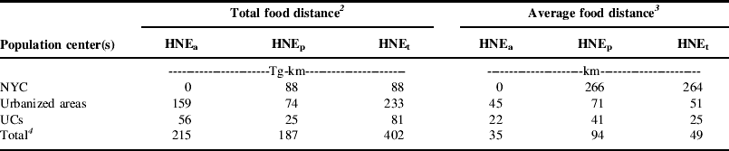
1 Quantities of food are expressed in weight of HNEs. An HNE is the amount of food needed to provide one person a complete diet that meets all nutritional requirements for 1 year. The diet is partitioned into food derived from annual and high-value crops (HNEa) and food derived from perennial forages (HNEp). Values are also shown for the total diet (HNEt). See text for more details.
2 Total food distance equals the weight of food supplied to a population center (or group of centers) times the distance traveled.
3 Average distance traveled equals the total food distance divided by the weight of food supplied to a population center (or group of centers).
4 Totals may not add due to rounding error.
In addition to the numerical summaries described above, data from the optimization model can be summarized visually by mapping foodsheds. To demonstrate this concept, the output matrix was used to delineate boundaries for potential local foodsheds for selected NYS population centers (Fig. 4). The background of each map shows the food production potential of all production zones, and the areas shaded in color indicate the production zones that supply food to a common population center. Only the six largest population centers are displayed as it is difficult to distinguish between more than six colors in a map. The shaded areas indicate the extent of each foodshed (the area covered), and the potential productivity (shown in gray scale) indicates where food comes from within the local foodshed. One interesting spatial pattern that separates the two maps is that little of the productive potential of HNEa was allocated to the NYC (purple) and Poughkeepsie–Newburgh (yellow) foodsheds, even though these cities have large populations. In contrast, the allocation of the available HNEp was more evenly distributed. This pattern reflects the fact that NYS has greater production potential of HNEp than HNEa, relative to food need, and therefore can supply more HNEp than HNEa to NYC and Poughkeepsie–Newburgh.

Figure 4. Maps of potential local foodsheds for the six largest population centers in NYS. Food production potential is shown in the background in grayscale. Areas shaded in color indicate the production zones allocated to a common population center (red=Buffalo, orange=Syracuse, yellow=Poughkeepsie–Newburgh, green=Rochester, blue=Albany, purple=NYC). Dots indicate the geographic center of the population center. (a) Foods derived from annual and horticultural crops (HNEa). (b) Foods derived from perennial forages (HNEp).
In cases where the potential local foodshed could meet all of the food needs of its population center, Rochester (shown in green) for example, the foodshed map gives an indication of the footprint of land required to support a city. However, since not all population centers could be fed in this model, it is helpful to examine not only the size of the foodshed but also the proportion of food needs it supplies (Fig. 5). For the purpose of displaying all foodsheds in a single map, the boundaries shown in Figure 5 aggregate production zones that primarily supply the same population center. The colors indicate the percentage of total food needs that are supplied within the potential local foodshed. Both the map of HNEa and the map of HNEp indicate that most population centers north and west of NYC could meet the majority of their food needs from the land within the state's borders. Those that are largely underfed in the model, like NYC, lie in the south east portion of the state.

Figure 5. Maps of potential local foodsheds for 125 NYS population centers indicating the percentage of each population center's food needs that could be supplied by the potential local foodshed. (a) Foods derived from annual and horticultural crops (HNEa). (b) Foods derived from perennial forages (HNEp).
Discussion
Models are simplifications of reality. Thus, to understand the implications of a model, the results must be placed in their proper context. The purpose of the foodshed model was to examine the capacity of individual population centers to secure their food needs locally. To achieve this goal, the food system was represented merely as a universe of producers and consumers. The only obstacle in the system was distance. In essence, the model determined how much of a population center's food supply could be ‘local’ based on where people live relative to where agriculture occurs.
Within this context, the results provide unique perspective on the capacity of NYS population centers to meet their food needs locally. Outside of the NYC area, most population centers could meet all, or nearly all, of their food needs within the State. In contrast, NYC goes almost completely unfed. This allocation makes sense, given the design of the model. The NYC population center lies in the southeast corner of the State, which has relatively little agriculture compared to the western half of the State. Thus, by virtue of its geography, NYC is poorly positioned to compete in a model that is designed to minimize the transport of food. Moreover, NYC has an enormous population, and even if it received all the available NYS production potential, it would meet just 55% of its total food needs. In a populous state like New York, not all food can be local.
Nonetheless, the results of the model suggest that NYS may be able to significantly reduce the distance food travels. The actual distance that food is transported through the food system is not known with certainty. However, it is frequently claimed (see, for example, Kloppenburg et al.Reference Kloppenburg, Hendrickson and Stevenson2, LappingReference Lapping50 and PrettyReference Pretty25) that food in the USA travels approximately 1300 miles (2080 km) from the farm to the consumer—a figure that appears to originate from a 1969 study of the US agricultural systemReference Brown and Pilz51. In contrast, both the urbanized areas outside of NYC and the UCs were able to provide the vast majority of their food needs within distances two orders of magnitude shorter than the oft cited 1300 mile figure. Since these population centers account for 37% of New York's population, it appears that food system re-localization has the potential to significantly reduce the distance food travels. However, the potential reduction would probably not be two orders of magnitude. As the results show, NYC accounted for 22% of the total food distance traveled even though it received just 4% of the total food (HNEt). Thus, were the geographic area expanded so that the food needs of NYC could be satisfied, it would have a profound influence on the average distance food travels. Given the food needs inherent in big cities relative to production potential in peri-UAs, feeding big cities may require food to travel great distances.
The application of the foodshed model in NYS imposes two limitations specific to the state's geography. First, the area of analysis lacked adequate production potential to meet the food needs of the resident population. This prevents the model from estimating the minimum distance within which all food needs could be supplied for all cities. Secondly, NYS is a relatively small geographic area, and the patterns observed in this analysis may only apply to regions with similar climate, land base, or population density. Thus, an obvious next step for foodshed research would be to apply the existing model to a larger, and more diverse, geographic area.
In addition to these geographic limitations, fundamental limitations are imposed by the way the model represents the food system. The model estimates the biophysical capacity of the land base to support food production in proportions that satisfy the nutritional needs of the resident population. However, this simplification of the food system differs from reality in three significant ways.
First, regions tend to specialize in certain types of agriculture, such as dairy, feed grains or orchard crops, whereas the model estimates production in HNEs, bundles of food in the proper proportions for a balanced diet. This prevents the model from focusing on foods that, for a variety of reasons, make sense to grow locally. For example, it may be possible for NYS to provide a greater share of its food needs, measured on a fresh-weight basis, by concentrating on foods with high water content such as fruits, vegetables and fluid milk.
Secondly, the model does not explicitly model the flow of food from its origin as an agricultural commodity at the farm gate through processing and distribution to its ultimate destination at the point of consumption. In general, this likely causes the model to underestimate the distance the food travels since the actual journey is more circuitous than simply traveling from farm to market. In addition, it requires the modeler to assume that the necessary processing infrastructure either exists or could be built within a given foodshed.
Thirdly, the model does not account for the influence of economic factors, such as economies of scale or comparative advantage, which can favor a more geographically extensive food system. These economic factors may provide a societal benefit by reducing the price of food for consumers, and the model presented here does not provide a means for analyzing such trade-offs.
One final limitation of this analysis is that the optimization goal, minimizing the distance food travels, is too simplistic to evaluate whether or not localization of the food supply is desirable for reducing greenhouse gas emissions or improving energy efficiency of the food system. Indeed, recent analysis suggests that ‘food miles’ are a poor indicator of environmental impactReference Edwards-Jones, Milá i Canals, Hounsome, Truniger, Koerber, Hounsome, Cross, York, Hospido, Plassman, Harris, Edwards, Day, Tomos, Cowell and Jones14. However, with additional data, the model could be adapted to optimize for either energy use or greenhouse gas emissions.
For all of the reasons listed above, the foodshed model presented here should be viewed as a first slice into the questions of how much food could and should be produced locally. Yet despite the limitations of this analysis, the foodshed model offers a flexible framework for answering questions that require one to consider the geography of food consumption and agricultural production simultaneously. As Peters et al.Reference Peters, Fick and Wilkins31 have argued, discussion of nutritional needs and agricultural production has proceeded along separate tracks, and tools are needed that help consider the two together. The model presented here provides such a tool. Moreover, it provides a platform that can be adapted to inform much broader questions of food security and environmental impact such as, ‘How might cities be fed as petroleum supplies peak and transportation becomes more expensive?’ or ‘How should the geography of the food system change to reduce its carbon footprint?’ Indeed, foodshed modeling may offer a valuable planning tool for creating more secure and less environmentally destructive food systems if we in the sustainability community can identify which issues would most benefit from geographic analysis.
Appendix: Layout of Optimization Problem
The optimization problem was set up in a single Excel® worksheet. This worksheet integrated the three major pieces of input data (production potential for each production zone, food needs of each population center, and the distance between production zones and population centers) with the optimization goal and constraints. A description of the spreadsheet design and its relationship to the equations noted in the text is given below.
The optimization worksheet can be broken into five major elements (see Table A1 for a general schematic). First, the five by six (rows×columns) matrix of empty cells located in the upper left quadrant of the table indicates the amount of food provided from each production zone to each population center. This ‘foodshed matrix’ contains one row for each production zone (1–5) and two columns for each population center (A, B and C), one for HNEa and a second for HNEp. Each cell in this matrix was a variable in the optimization problem, meaning that the optimization software searched for the appropriate set of values for these cells that minimized food distance, within certain constraints.
Table A1. Generalized layout of the optimization problem used in the foodshed model.Footnote 1

1 Meaning of symbols is defined in footnotes 2 through 8. See the text for a complete description of this table.
2 The abbreviation HNE stands for Human Nutritional Equivalents. Subscripts ‘a’ and ‘p’ indicate, respectively, foods derived from annual and high value crops and foods derived from perennial forages. See Methods section for complete definitions.
3 Nomenclature shown indicates the sum (Σ) of the food (F) from a given food category (a or p) that has been allocated by a given production zone (1 through 5).
4 Nomenclature shown indicates the food production potential (P) of a given production zone (1 through 5) for growing food from a given food category (a or p).
5 Nomenclature shown indicates the sum (Σ) of the food (F) from a given food category (a or p) that has been allocated to a given population center (A through C).
6 Nomenclature shown indicates the food needs (C) of a given population center (A through C) from a given food category (a or p).
7 Nomenclature shown indicates the sum (Σ) of the product of the quantity of food (F) from each food category (i) allocated by each production zone (j) to each population center (k) and the distance (D) between each production zone and population center.
8 Nomenclature indicates the distance (D) between each production zone (1 through 5) and population center (A through C).
Secondly, the four columns to the right of the foodshed matrix were used to constrain the model to allocate all available production potential (see Eqn 4b). The cells in the two leftmost columns calculate the total food allocated from each food category by each production zone (∑F ij), corresponding to the left-hand side of Equation 4b. The cells in the two rightmost columns contain estimates of the total production potential of each production zone (P ij), corresponding to the right-hand side of Equation 4b and calculated as shown in Equation 1.
Thirdly, the two rows directly below the foodshed matrix were used to prevent the model from exceeding the food needs of each population center (see Eqn 4a). The upper row of cells calculate the total amount of food from each category that has been allocated to each population center (∑F ik), corresponding to the left-hand side of Equation 4a. The lower row contains estimates of the total food needs from each food category for each population center (C ik), corresponding to the right-hand side of Equation 4a and calculated as shown in Equation 2.
Fourthly, the five by six (rows×columns) matrix located in the lower left quadrant of the table contains estimates of the distance between each production zone and each population center (D jk). This distance matrix was calculated as described in the Methods section.
Fifthly and finally, the bordered cell labeled ‘food distance’ calculated the total food distance traveled by multiplying the values shown in the foodshed matrix by those in the distance matrix (∑F ijk×D jk). This cell corresponds to the right-hand side of Equation 3. This cell is the value that the model seeks to minimize by iteratively changing the values in the foodshed matrix.
The schematic in Table A1 shows a generalized version of the optimization worksheet developed in Excel®. The actual optimization problem developed for the foodshed model was much larger. It included 5385 production zones, 125 population centers and two categories of food. Thus, the actual foodshed matrix contained a grand total of 1,346,250 variables. The limits placed on the total food that could be produced by each production zone or received by each population center created a total of 11,020 constraints. The size of this problem necessitated the use of the Premium Solver Platform™ v6.5 and the Extended Large-Scale LP Solver Engine v6.5 from Frontline Systems42, 43.
Acknowledgements
This research was supported in part by the National Research Initiative of the USDA Cooperative State Research, Education and Extension Service, grant number 2005-55618-15640.