Introduction and background

Much of agricultural production in the United States (US) is attributed to larger, monoculture or commodity crop production. Mid-sized and large-scale family farms account for the majority of the revenues in the US (60%), but only 8% of all US farms (Hoppe, Reference Hoppe2014). Larger operations are generally able to realize lower costs due to economies of scale associated with farming and ranching. These economies of scale are significantly influenced by technological and structural change in the industry and are positively associated with financial viability (MacDonald and McBride, Reference MacDonald and McBride2009). Although small family farmsFootnote ¹ produce only 26% of the value of farm output, they represent 90% of US farms. Further, they are much less likely to be profitable compared with larger-sized operations, and thus attention to their economic viability is key to the resiliency of the sector (Hoppe, Reference Hoppe2014). This study seeks to explore the financial efficiency of farms and ranches who participate in direct markets, a sector dominated by small operations.

Digging deeper into differences in the financial indicators of small farms compared with midsizedFootnote ² and largeFootnote ³ family farms, we note some key discrepancies. Small family farms are much more likely to have tight financial margins making it much more difficult to weather market or production shocks. Hoppe (Reference Hoppe2014) shows that small farms are more likely to have a rate of return on assets (ROA)Footnote ⁴ of <1% and an operating profit margin of <10%; which he defines as the ‘critical zone’. One mechanism that small farms have found to deal with scale diseconomies is through off-farm income. Small farm operators have a much larger reliance on these non-farm sources of income and can thus be less reliant on the farm's returns for their household's economic well-being (Fernandez-Cornejo et al., Reference Fernandez-Cornejo, Mishra, Nehring, Hendricks, Southern and Gregory2007; Hoppe, Reference Hoppe2014).

Another opportunity for small producers may be adding value post-farmgate, through participating in consumer-focused, value-added and direct markets (Bauman e t al., Reference Bauman, Thilmany and Jablonski2017). These markets require producers to take on more supply chain functions, including marketing, processing and distribution; in return, they are able to retain a larger portion of the retail dollar (King et al., Reference King, Hand, DiGiacomo, Clancy, Gomez, Hardesty, Lev and McLaughlin2010). In 2015, 167,000 operations sold through direct marketing channels, including direct-to-consumer sales (e.g., farmers’ markets) and intermediated channels (e.g., farm-to-restaurant, farm-to-school), and accounted for $8.7 billion in sales (USDA NASS, 2016). In recent years, the growth in local food marketing channels has been significant. For example, between 2006 and 2014, farmers’ markets have grown 180% and food hubs by 288% (Low et al., Reference Low, Adalja, Beaulieu, Key, Martinez, Melton, Perez, Ralston, Stewart, Suttles, Vogel and Jablonski2015).

Most of the economic research on local food systems has focused post-farmgate including supply chain analysis (e.g., King et al., Reference King, Hand, DiGiacomo, Clancy, Gomez, Hardesty, Lev and McLaughlin2010; Hardesty et al., Reference Hardesty, Feenstra, Visher, Lerman, Thilmany McFadden, Bauman and Rainbolt2014), economic impact studies (e.g., Hughes et al., Reference Hughes, Brown, Miller and McConnell2008; Brown et al., Reference Brown, Goetz, Ahearn and Liang2014; Jablonski et al., Reference Jablonski, Schmit and Kay2016, Schmit et al., Reference Schmit, Jablonski and Mansury2016) and consumer-oriented factors that have driven the demand for local food (e.g., Lusk and Briggeman, Reference Lusk and Briggeman2009; Onozaka and Thilmany, Reference Onozaka and Thilmany McFadden2011; Costanigro et al., Reference Costanigro, Kroll, Thilmany and Bunning2014).

There is very little research that examines the farm financial outcomes associated with sales through these channels. Nor is there adequate ‘peer’ data that allow local food producers to compare themselves with similar farms or to provide a roadmap for strengthening financial viability or planning for market growth. Yet, farmers and ranchers, the US Department of Agriculture (USDA), lenders and private foundations that fund regional food systems have an interest in understanding how new markets influence the resiliency of farms. Particularly, understanding the financial well-being of beginning or smaller operations for whom more traditional commodity-oriented markets may have larger barriers to entry (e.g., Farm Credit Administration, 2016; Thilmany McFadden et al., Reference Thilmany McFadden, Bauman and Jablonski2016a, Reference Thilmany McFadden, Conner, Deller, Hughes, Meter, Morales, Schmit, Swenson, Bauman, Phillips Goldenberg, Hill, Jablonski and Troppb). Access to and consideration of this comparative information is one promising approach to better understand their competitive position, and if needed, consider factors influencing their profitability.

From the standpoint of the USDA and private foundations that provide funding in this area, understanding the factors that influence efficiency will enable them to better target their resources and support local and regional food system development. As one example, the Farm Service Agency is striving to provide more capital to farms participating in these markets, but needs to understand the underlying factors that allow farms to be viable (and repay their loans) (USDA FSA, Reference Wolf, Stephenson, Knoblauch and Novakovic2016). Additionally, in 2015, the USDA Risk Management Agency began piloting Whole-Farm Revenue Protection, a program that provides an insurance plan for diversified producers selling through local and regional food markets (USDA RMA, 2017). In both cases, for financing and risk management programs to be structured effectively, a better understanding of the determinants of efficiency will be important.

To our knowledge, there have been no studies that focus on the financial performance and efficiency of farming operations that participate in both the direct and intermediated marketing channels. This research explores: how does the financial performance of farms utilizing local food markets compare to their peers? Does the optimal size vary among farmers depending on the nature of how they participate in the local food system? Is there an optimal diversification strategy with respect to market orientation, or is that dependent on other factors (cost structure, scale, region, primary commodity)?

The goal of this paper is threefold: first, to ascertain the average (and comparative) efficiency levels of farm operations that participate in direct and intermediated markets; second, to identify the factors that have the greatest influence on the relative efficiency of farms and ranches that participate in local food systems; and finally, to estimate the relationship between marketing strategy and farm profitability and productivity, with a particular focus on the role of farm size. We build on Park (Reference Park2015), utilizing more recent data (with larger sample sizes of local food producers) and different methods with a focus on efficiency impacts within the direct market sector only.

Previous research on direct marketing farm financial outcomes

Given the well-documented evidence of consumer willingness to pay a premium for products sold through direct markets (e.g., Onozaka and Thilmany, Reference Onozaka and Thilmany McFadden2011; Costanigro et al., Reference Costanigro, Kroll, Thilmany and Bunning2014), one must understand differential expenditure patterns associated with sales through these markets. There are only a handful of case studies that examine differential farm expenditures and sales by market channel (Hardesty and Leff, Reference Hardesty and Leff2010; LeRoux et al., Reference LeRoux, Schmit, Roth and Streeter2010; Jablonski and Schmit, Reference Jablonski and Schmit2016). These three studies examine the differential expenditures per unit of sales by market channel, paying particular attention to labor and fuel utilization. However, the sample size is small in each of these studies as they required primary data collection. Thus, past studies did not integrate methods that allow for rigorous comparison or analysis.

Jablonski and Schmit (Reference Jablonski and Schmit2016) did compare their case studies to USDA, Agricultural Resource Management Survey (ARMS) data, however it was only for New York, for which the ARMS sample is relatively small. Literature examining farm financial outcomes for local food market participants is mixed. Low et al. (Reference Low, Adalja, Beaulieu, Key, Martinez, Melton, Perez, Ralston, Stewart, Suttles, Vogel and Jablonski2015) use USDA ARMS data to conduct a preliminary exploration of the financial impacts of sales through direct markets. They find that, on one hand, farms who participate in direct markets, regardless of scale, are significantly more likely to survive (defined by the USDA as a farm business having positive sales in subsequent census, 2007 and 2012) than farms who market through more traditional, commodity market channels. However, farms with gross cash farm income (GCFI) >$10,000 grew at a significantly slower pace during the same period than farms who used traditional markets.

Park (Reference Park2015) uses national-level data and finds that, compared with traditional marketing channels, participating in direct markets has a negative impact on farm sales (which lessens as farm size increases). Detre et al. (Reference Detre, Mark, Mishra and Adhikari2011) examines factors affecting the adoption of direct marketing strategies and its impact on gross sales using 2002 ARMS data. Results show that farms who adopt direct marketing strategies capture a larger proportion of the consumer dollar, thus increasing gross sales, compared to those using more traditional sales channels (such as large scale, commodity distributors).

Part of the reason for limited previous research on local foods markets is that national data were limited until very recently. Although national data on direct-to-consumer sales have been available since 1976 in the census, intermediated sales by farm operators have only been available since 2008, when the ARMS began collecting these data. As intermediated sales represent the largest segment of local food sales, analysis before 2008 was incomplete. In a congressionally mandated report on Trends in Local and Regional Food Systems, Low et al. (Reference Low, Adalja, Beaulieu, Key, Martinez, Melton, Perez, Ralston, Stewart, Suttles, Vogel and Jablonski2015) were only able to provide what they call ‘a synthetic estimate of local food sales values’ due to data deficiencies, illustrating the challenge. The ARMS now provides a sufficiently large sample of financial data for producers participating in local food systems at the national level, allowing for a more rigorous financial assessment of this subset of US farmers.

Empirical approach

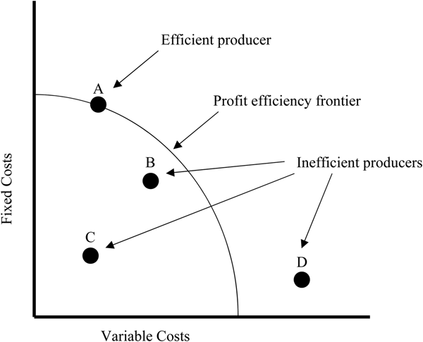
The most common approach to estimating production or financial efficiency across the farm sector is stochastic frontier analysis (SFA)Footnote ⁵, whereby a production/cost/profit function is estimated with an error composed of both a productive inefficiency component and a random component. It is assumed that the production/cost/profit function is the theoretical ideal, mapped endogenously against those firms included in the data (peer direct market farms), so any deviation from this function is the result of an inefficiency (Green, Reference Green2012). Figure 1 describes a profit efficiency frontier. Input costs are on the x- and y-axes and a profit frontier is estimated, representing the combination of fixed and variable input costs that produce the highest profit. Producers that lie above or below the profit frontier could earn higher profits using a different combination of fixed and variable inputs, and are thus considered inefficient. Those producers who lie on the efficiency frontier are efficiently using inputs to create profit and would not increase profits if they were to shift their spending on fixed and variable inputs.

Fig. 1. Profit efficiency frontier.

Although there have been no studies that evaluate the efficiency of local and regional food system participants, there have been numerous studies that use SFA to evaluate the efficiency of other types of US farming and ranching operations (e.g., Morrison and Nehring, Reference Morrison Paul and Nehring2005; Mayen et al., Reference Mayen, Balagatas and Alexander2010; Key and McBride, Reference Key and McBride2014), as well as international farming and ranching operations (e.g., Bokusheva et al., Reference Bokusheva, Hockmann and Kumbhakar2012; Barath and Ferto, Reference Barath and Ferto2015). SFA allows us to estimate the maximum attainable output/profit for a given set of inputs and prices. By additionally including farm characteristics in our model beyond, we are able to determine the full set of factors that likely influence a producer's ability to reach this ideal.

We estimate a profit frontier where profit is defined as ROA. Lack of data precludes estimation of an output function, so the remaining choices for this study were estimating either a profit or a cost function. The choice to use a profit function was based on a couple of factors given the context of this sector and study. The more commonly employed cost functionFootnote ⁶, focused on estimating cost inefficiency, does not enable us to capture the effects of the business strategy to focus on higher quality output one might expect farmers to market in highly differentiated markets. This is important as we assume such a quality-focused strategy would be more costly, but not necessarily inefficient if price premia offset additional costs of differentiation. By estimating a profit frontier we can capture differentiation as the key specialization strategy, allowing the producers that produce higher quality outputs to compensate for the higher costs that they incur in the production process through increased revenue earnings (Maudos et al., Reference Maudos, Pastor, Pérez and Quesada2002). Another reason to focus on ROA rather than costs, or even operating profitFootnote ⁷, is because it standardizes against one key metric: invested assets.

ROA is a commonly used metric to evaluate farm profitability and is calculated by dividing net income by total assets. It measures how efficiently a firm can create profit using their invested assets in a given year, accounting for the opportunity cost of money. Although not commonly used in profit frontier estimation, the use of a ‘standardized’ measure like ROA may allow some expected and interesting cases (such as lean management farms with few owned assets that compete through aggressively pursuing high end produce and product markets) to emerge more clearly (e.g., Ho et al., Reference Ho, Newman, Dalley, Little and Wales2013; Wolf et al., Reference Wolf, Stephenson, Knoblauch and Novakovic2016). In contrast, gross measures, such as operating profit, may mask some interesting aspects of farms participating in direct markets. In short, since ROA represents the profitability and returns relative to the dollar value of assets invested in the farm, it allows farms that may have adopted ‘lean’ management strategies (minimal overhead) to stand out as particularly strong performing. Given the local food sector's inclusion of beginning, small or limited resource farms, such a metric where farms can rely on rented rather than owned assets may be of particular interest.

The main challenge associated with this approach is the existence of negative profits; one cannot take the natural log of a negative value. This challenge is not applicable in traditional SFA in which a production or a cost frontier is estimated as output and cost are always positive. Accordingly, results presented herein represent only the information provided by those farms with a positive value of ROA. Explanatory variables include variable and fixed expenses, operator age, education, market outlet, scale, primary commodity, year, off-farm income and per cent of farmland that is owned.

Using SFA allows us to disentangle the effect of scale on efficiency from the many other factors that influence efficiency, a particular focus here given the perceptions by policymakers and government agencies that local and regional food systems are particularly important business opportunities for smaller scale producers. In our study, we use GCFI as a proxy for scale. Marketing channel and scale can be interdependent factors, as larger producers in local food systems generally sell through intermediated marketing channels while smaller producers usually sell through direct-to-consumer marketing channels. But, these differences are not necessarily clear and distinct. To disentangle the effects that scale and marketing channel may have on efficiency, the model is estimated with both included, and then again for comparative purposes, with only the marketing channel variables and only scale included. In addition to marketing channel, primary commodity may also have an influence on financial efficiency. While fruit and vegetable producers make up the majority of sales for producers in local food systems (Low and Vogel, Reference Low and Vogel2011; Low et al., Reference Low, Adalja, Beaulieu, Key, Martinez, Melton, Perez, Ralston, Stewart, Suttles, Vogel and Jablonski2015) profitability has been shown to vary across output types (Detre et al., Reference Detre, Mark, Mishra and Adhikari2011).

Previous literature also points to the impact that farm characteristics such as operator age, operator education and reliance on off-farm income may have on efficiency. Younger operators have higher debt than older operators and typically finance farming operations through borrowed capital (Mishra et al., Reference Mishra, El-Osta, Morehart, Johnson and Hopkins2002). Park et al. (Reference Park, Mishra and Wozniak2014) found that younger farmers were more likely to participate in direct marketing channels than older farmers, likely due to the fact that accessing local and regional food markets may require less production volume and/or capital than gaining access to traditional agricultural markets.

In studies of producers using traditional market outlets, operator education typically increases farm household income (e.g., Mishra et al., Reference Mishra, El-Osta, Morehart, Johnson and Hopkins2002). In local and regional food systems, there may be a greater reliance on aggressively managed marketing and operations compared with traditional market outlets because managers feel a need to gain the highest return possible on their more limited volume of production. If this is the case, operator education is likely to have an impact on these producers in local and regional food systems, and possibly even more so than those producers utilizing traditional marketing channels. Indeed, Park et al. (Reference Park, Mishra and Wozniak2014) finds that operators with a broader portfolio of marketing skills are more likely to increase farm sales relative to farmers who are using fewer marketing skills, indicating the importance of education on efficiency. More than half of all US farm households have a household member that works off-farm (Mishra et al., Reference Mishra, El-Osta, Morehart, Johnson and Hopkins2002) and the same is true for producers participating in local and regional food systems (Low and Vogel, Reference Low and Vogel2011). Given the reliance on off-farm income, it is likely to be an important factor in determining profitability, as found by Park et al. (Reference Park, Mishra and Wozniak2014). However, it may also compete with time spent focused on the agricultural enterprise, therein representing a challenge to managerial efficiency.

Econometric model

We estimate the factors that have the greatest impact on the technical efficiency of local food system participants using SFA, first proposed by Aigner et al. (Reference Aigner, Lovell and Schmitt1977) and Meeusen and van den Broeck (Reference Meeusen and van den Broeck1977). The model has the form:

$$\ln \left( {{\pi} _i} \right) = f\left( {x_i,{\rm \beta}} \right) + v_i - u_i$$

where π_i is the profit for producer i, and f(x _i, β) is the maximum profit that can be obtained with the vector of logged inputs, x _i, and the technology described by the parameters β. Deviation from the maximum profit for an individual can either be from a random shock, v _i or due to a production inefficiency, u _i, where u _i ≥ 0. The production function for an individual is specified as a second-order translog function such that $f\left( {x_i,{\rm \beta}} \right) = {\rm \beta} _0 + \sum\nolimits_{k = 1}^K {{\rm \beta} _k{\rm ln}(x_{ik}) + \displaystyle{1 \over 2}} \sum\nolimits_{k = 1}^K {\sum\nolimits_{j = 1}^{} {{\rm \beta} _{kj}\ln \left( {x_{ik}} \right){\rm ln}(x_{ij})}} $,Footnote ⁸ where β₀ is the constant and β_k are the coefficients for each of the k independent variables.

The technical efficiency for an individual producer is defined as the ratio of the observed profit of an individual producer to the maximum observed profit:

$$TE_i = \displaystyle{{{\pi} _i} \over {{\rm exp}\left( {\,f\left( {x_i,{\rm \beta}} \right) + v_i} \right)}} = {\rm exp}\left( { - u_i} \right)$$

where 0 ≤ TE _i ≤ 1. When TE _i = 1, the producer is on the efficiency frontier while for any TE _i < 1 the producer falls below the efficiency frontier.

We assume the commonly utilized normal/half-normal distribution in which v _i is distributed $N\left( {0,{\rm \sigma} _v^2} \right)$, u _i is distributed $N^ + \left( {0,{\rm \sigma} _u^2} \right)$, v _i and u _i are statistically independent of each other, and v _i and u _i are independent and identically distributed across observations. Given this distribution $E\left[ u \right] = {\rm \sigma} _u\sqrt {2/{\rm \pi}} $ and ${\rm var}\left[ u \right] = {\rm \sigma} _u^2 \left[ {\left( {{ \pi} - 2} \right)/{\pi}} \right]$, where 0 <u _i <∞. The log-likelihood function is as follows:

$${\rm ln} \, L\left( {{\pi} \vert {\rm \beta}, {\rm \lambda}, {\rm \sigma} ^2} \right) = \mathop \sum \limits_{i = 1}^N \left\{ {\displaystyle{1 \over 2}\ln \left( {\displaystyle{2 \over { \pi}}} \right) - {\rm ln}{\rm \sigma} + {\rm ln\Phi} \left( {\displaystyle{{ - {\rm \varepsilon} _i{\rm \lambda}} \over {\rm \sigma}}} \right) - \displaystyle{{{\rm \varepsilon} _i^2} \over {2{\rm \sigma} ^2}}} \right\}$$

where ${\varepsilon} _i = {\pi} _i - x_i^{\rm ^{\prime}} {\rm \beta, \lambda} = {\rm \sigma} _u/{\rm \sigma} _v,{\rm \sigma} = \left( {{\rm \sigma} _u^2 + {\rm \sigma} _v^2} \right)^{1/2}$ and Φ is the standard normal cumulative distribution function (Aigner et al., Reference Aigner, Lovell and Schmitt1977).

The main parameter of interest, u _i, is the technical efficiency of each individual enterprise, which is a component of the estimated error, ε _i = v _i + u _i. As u _i is not directly estimable, to assess the technical efficiency for an individual enterprise, we estimate the expected value of u _i given ε _i:

$$E\left( {u_i \vert {\rm \varepsilon} _i} \right) = {\rm \mu} _{{\ast}i} + {\rm \sigma} _{\ast}\left\{ {\displaystyle{{{\phi} \left( { - {\rm \mu} _{{\ast}i}/{\rm \sigma} _{\ast}} \right)} \over {{\rm \Phi} \left( {{\rm \mu} _{{\ast}i}/{\rm \sigma} _{\ast}} \right)}}} \right\}$$

where ${\rm \mu} _{*i} = {\rm \varepsilon} _i{\rm \sigma} _u^2 /{\rm \sigma} ^2,{\rm \sigma} _* = {\rm \sigma} _u{\rm \sigma} _v/{\rm \sigma} $, and ϕ is the standard normal probability density function (StataCorp, 2013).

Data

Data are taken from the 2013 and 2014 Phase III ARMS to estimate the parameters of the model. The data include GCFI, marketing channels utilized, primary commodity, fixed and variable expenses, assets, debt, and farm and operator characteristics. The ARMS is a nationally representative survey that targets about 30,000 farms annually and utilizes a complex survey design (e.g., complex stratified, multiple frame and probability weighted). It is the most comprehensive national source of farm financial data (Low and Vogel, Reference Low and Vogel2011). The ARMS mission is to provide annual, national-level data on farm business with a particular focus on 15 core agricultural states. Therefore, it may provide a relatively small sample of a niche group, such as direct market producers, particularly in the non-core agricultural states. Although the ARMS is not designed to specifically collect data on agricultural sectors such as direct marketing, it does integrate questions on this sector and remains the best source of nationally representative data available for this type of analysis (Low and Vogel, Reference Low and Vogel2011; Low et al., Reference Low, Adalja, Beaulieu, Key, Martinez, Melton, Perez, Ralston, Stewart, Suttles, Vogel and Jablonski2015).

Given this survey design, if the purpose of the analysis is to describe the population, then the estimates must be weighted (using a jackknife weighting scheme as recommended by the USDA Economic Research Service). But, if the purpose is to describe variability within a sample (in our case farms and ranches selling through local food marketing channels), then weighting the sample will distort the results by forcing this sample to appear more like the average farm or ranch (Dubman, Reference Dubman2000). In other words, if the goal is to compare farms and ranches selling through local food markets to those farms and ranches utilizing traditional marketing channels, then it is necessary to weight estimates. But, as is the case in this paper, if the comparison is within local food marketing channels, then no weighting is necessary.

By not using the jackknife weighting scheme to standardize the sample analyzed, this paper assumes that: (1) local food producers would not be shown as representative using the criteria commonly used to create more representative farms in the ARMS sampling scheme; (2) the ARMS sampling scheme is representative of all farms so comparisons of our targeted set of producers to the sample still offers some important inferences. We did not modify the targeted sample to normalize it to a representative US farm population because we expect it is the direct marketing farms’ variance from being ‘representative’ that is interesting for comparisons.

In the ARMS data collection protocol, sales through local food markets are asked in two ways (similar to how questions are asked in the Census of Agriculture). First, participants are asked to respond (yes/no) if they produced, raised or grew commodities for human consumption that were sold directly to: (1) individual consumers, (2) retail outlets or (3) institutions. Subsequently, they are asked to provide how much money was received for the cash market, open market or marketing contract sales from selling; (1) directly to consumers at farmers markets, (2) directly to consumers from on-farm store, u-pick, roadside stands, CSAs, (3) to a local retail outlet such as a restaurant or grocery store, (4) to a regional distributor such as a food hub or (5) to a local institutional outlet such as a school or hospital. We define local food system participants as all those that reported positive sales in any of the five direct marketing channels listed above.

Following Low et al. (Reference Low, Adalja, Beaulieu, Key, Martinez, Melton, Perez, Ralston, Stewart, Suttles, Vogel and Jablonski2015), sales to individual household consumers are classified as direct-to-consumer sales, while sales to retail outlets and institutions are classified as intermediated sales. Of the total sample, 41,912 (94%) reported no local food sales and 2624Footnote ⁹ (6%) responded that they had positive sales in any combination of local food marketing channels. For all those respondents who reported positive sales in local food marketing channels, 1690 (64%) had positive direct-to-consumer sales only, 380 (15%) had positive intermediated sales only and 554 (21%) had positive sales to both outlets. Table 1 provides summary statistics for the main variables used in the study, reported as an aggregate across all sales categories as well as broken out by sales category.

Table 1. Summary statistics for local food farmers and ranchers

¹ 1: ⩽34, 2:35–44, 3:45–54, 4:55–34, 5:65+.

² 1: less than high school, 2: completed high school, 3: some college, 4: completed 4 yr of college or more.

As a whole, farms participating in direct marketing channels show a broad range of profitability with farms over $350,000 in sales reporting an average ROA of over 10%, a strong result for a generally low margin industry such as agriculture. Fixed expenses as a portion of total expenses decrease with scale, ranging from 31% for producers with sales between $1000 and $74,999 to 15% for producers with sales over $350,000. This is what we would expect and demonstrate one of the benefits of scaling up. Variable expenses as a percentage of total expense follow an opposite trend, increasing from 69 to 85% as scale increases from $1000–$74,999 to over $350,000. Labor expense as a portion of total expense increases with scale, ranging from 7 to 32%. This greater reliance on labor could demonstrate a shift from operator and unpaid labor into paid labor and/or an increase in the reliance on more hours and skills within a labor force for specialized production and marketing activities as the size and complexity of a farming enterprises increases.

On average, producers are in the age range of 45–54 and have completed high school. The portion of acres owned to farm is 1.2 for the smallest scale producers; so on average, these producers own more land than they farm. As scale increases, producers own less and lease more land, providing evidence that most producers scale up by leasing land rather than purchasing new land. This is one example we might expect to see if a farm was taking a ‘lean’ management approach. As was found to be the case with all small farms (Fernandez-Cornejo et al., Reference Fernandez-Cornejo, Mishra, Nehring, Hendricks, Southern and Gregory2007), small direct market producers rely more heavily on off-farm income compared with mid-size and large farms.

On average, 64% of producers participate in direct-to-consumer marketing channels only, 15% in intermediated only and 21% in both types of channels. Scale and participation in market channels show expected results: small-scale producers mostly participate in direct-to-consumer marketing channels and as scale increases, producers participate in intermediated marketing channels. In terms of primary commodity, 34% of producers sell fruits and vegetables, 19% field crops and 41% livestock. The portion of fruit and vegetable production is relatively constant across scale categories, but small-scale producers are more likely to produce livestock, whereas larger producers are more likely to produce field crops.