INTRODUCTION
In radiocarbon (14C) dating it is crucial to know which carbon reservoirs were involved in the formation of a sample. Samples that were formed in equilibrium with the atmospheric reservoir will produce a 14C age that represents the concentration of 14C in the atmosphere at that time. However, samples with carbon from marine or freshwater reservoirs will contain lower concentrations of 14C, making the sample appear older than it truly is. The difference between the 14C age of a sample originating from a fully atmospheric reservoir and the 14C age of a sample with carbon from a marine or freshwater reservoir is called the reservoir age. The situation can be complicated further in certain aquatic environments, such as the Limfjord in northern Denmark, which changed considerably over the last 7000 years, thus affecting the reservoir ages as well (Philippsen et al. Reference Philippsen, Olsen, Lewis, Rasmussen, Ryves and Knudsen2013). Correcting 14C ages of archaeological human and animal bone collagen samples for reservoir offsets requires an estimation of the percentage marine protein intake if marine resources were present in the consumers’ diets. δ13C values have been used in regions dominated by C3 plants since the δ13C values of terrestrial plants and animals are lower than for marine organisms. Using the δ13C value of the analyzed individual, the amount of marine protein intake, and thus carbon with an older apparent age, can be estimated and the radiocarbon age can be corrected for potential reservoir effects. However, marine protein consumption can be masked in terms of the δ13C values in a low protein diet (Hedges Reference Hedges2004). In such a diet, carbon can be (partially) derived from carbohydrates and lipids instead of a protein source (e.g. meat, fish, plants), which can result in “scrambled routing” of the carbon. As a result, the δ13C values in bone collagen may be less enriched than expected, which would have consequences for the reservoir correction of the 14C age of humans or animals consuming marine protein. δ13C values in marine fauna can also be influenced by freshwater input (Craig et al. Reference Craig, Ross, Andersen, Milner and Bailey2006), which could subsequently affect consumers as well. In regions with C4 plants, it may be difficult to distinguish between marine and terrestrial protein. δ15N values can be used instead of δ13C values because protein consumption results in elevation of δ15N values in bone collagen (Schoeller Reference Schoeller1999). Because the marine environment has more trophic levels than the terrestrial food chain, marine protein intake would result in more elevated δ15N values in the consumers compared to a fully terrestrial diet. However, there are factors other than diet that can affect δ15N values, such as soil composition (Heaton Reference Heaton1987; Britton et al. Reference Britton, Müldner and Bell2008) and fertilization activities (Koerner et al. Reference Koerner, Dambrine, Dupouey and Benoit1999; Choi et al. Reference Choi, Ro and Hobbie2003; Bogaard et al. Reference Bogaard, Heaton, Poulton and Merbach2007, Reference Bogaard, Fraser, Heaton, Wallace, Vaiglova, Charles, Jones, Evershed, Styring, Andersen, Arbogast, Bartosiewicz, Gardeisen, Kanstrup, Maier, Marinova, Ninov, Schäfer and Stephan2013; Fraser et al. Reference Fraser, Bogaard, Heaton, Charles, Jones, Christensen, Halstead, Merbach, Poulton, Sparkes and Styring2011; Kanstrup et al. Reference Kanstrup, Thomsen, Andersen, Bogaard and Christensen2011, Reference Kanstrup, Holst, Jensen, Thomsen and Christensen2014; Szpak Reference Szpak2014). Additionally, it is unclear to what extent individual variation relating to internal processes, such as metabolism, physiology and stress, can be observed in δ15N values (Schoeller Reference Schoeller1999; Hedges and Reynard Reference Hedges and Reynard2007). It is generally assumed that humans and animals are overall in a steady state, apart from periods of serious illness (Fuller et al. Reference Fuller, Fuller, Sage, Harris, O’Connell and Hedges2005; Mekota et al. Reference Mekota, Grupe, Ufer and Cuntz2006), intense growth or pregnancy (Schoeller Reference Schoeller1999; Fuller et al. Reference Fuller, Fuller, Sage, Harris, O’Connell and Hedges2004), because the nitrogen balance in the body might change in these conditions and affect the δ15N values. Having another proxy besides δ13C or δ15N values to estimate marine dietary intake would be advantageous in order to calculate accurate reservoir correction of 14C ages. As such, the aim of this study was to test the use of δ2H values to quantify the marine protein intake and determine the reservoir corrections.
Hydrogen
Hydrogen stable isotope analysis has routinely been applied to keratin-based tissues, such as hair, in forensic and even archaeological contexts (Sharp et al. Reference Sharp, Atudorei, Panarello, Fernández and Douthitt2003), as well as feathers in animal migration studies (Nelson et al. Reference Nelson, Braham, Miller, Duerr, Cooper, Lanzone, Lemaître and Katzner2015), while only a few studies using archaeological bone material have been published (Reynard and Hedges Reference Reynard and Hedges2008; Arnay-de-la-Rosa et al. Reference Arnay-de-la-Rosa, González-Reimers, Velasco-Vázquez, Romanek and Noakes2010; Gröcke et al. Reference Gröcke, Sauer, Bridault, Drucker, Germonpré and Bocherens2017; van der Sluis et al. Reference van der Sluis, Hollund, Kars, Sandvik and Denham2016). As with oxygen, hydrogen shows a strong connection with precipitation values, which are in turn linked to latitude, altitude, and continentality (Meier-Augenstein et al. Reference Meier-Augenstein, Hobson and Wassenaar2013). However, δ2H values also show good correlation with δ15N values and can thus be considered an additional trophic level indicator (Birchall et al. Reference Birchall, O’Connell, Heaton and Hedges2005; Peters et al. Reference Peters, Wolf, Stricker, Collier, Martinez and del Rio2012). Because δ15N values can be influenced by a number of factors other than protein consumption, hydrogen can prove to be a useful tool in establishing trophic level. Since the mass difference between 1H and 2H is 100%, the trophic level differences are much larger compared to carbon and nitrogen. While absolute δ2H values of an individual are linked to geographic location, relative difference between consumers show similar increases per trophic level (30–50‰ for herbivores to omnivores and 10–20‰ from omnivores to humans) (Reynard and Hedges Reference Reynard and Hedges2008). Body size can have an effect on δ2H values, resulting in long-term averaged values in large mammals and short-term values in small rodents, which might reflect seasonal climate and/or environmental influences (Topalov et al. Reference Topalov, Schimmelmann, Polly, Sauer and Lowry2013). While δ2H values are controlled by both drinking water as well as ingested foods, it is thought that the hydrogen in protein-based tissues is largely derived from the diet rather than from water (Sharp et al. Reference Sharp, Atudorei, Panarello, Fernández and Douthitt2003; Bowen et al. Reference Bowen, Ehleringer, Chesson, Thompson, Podlesak and Cerling2009). This reduced effect of drinking water on δ2H values might be connected to the slow turnover rate of bone collagen (Topalov et al. Reference Topalov, Schimmelmann, Polly, Sauer and Lowry2013).
Hydrogen in bone collagen consists of a non-exchangeable (~79%) and an exchangeable (~21%) fraction, the latter consisting of so-called labile hydrogen atoms that are bound to functional groups, e.g. -NH2, -OH and -COOH (Reynard and Hedges Reference Reynard and Hedges2008; Meier-Augenstein et al. Reference Meier-Augenstein, Hobson and Wassenaar2013). The exchangeable fraction quickly equilibrates with hydrogen values from the burial and subsequently laboratory environment, resulting in meaningless values. The δ2H values of this fraction needs to be determined in order to obtain that of the non-exchangeable fraction, which contains the original, true δ2H values. This is done using a 2-stage equilibration method, in which each original sample is divided into two subsamples (A and B), which are equilibrated with two water standards of known isotopic value (Bowen et al. Reference Bowen, Chesson, Nielson, Cerling and Ehleringer2005). This will produce two sets of samples, one set with exchangeable fractions equilibrated with water A and the other with water B. These two equilibration waters need to differ by at least 100‰. By applying this 2-stage equilibration method, sample specific and process specific factors influencing exchange rates are compensated for and we assume that the stable isotope ratio of the exchangeable hydrogen is fixed (Meier-Augenstein et al. Reference Meier-Augenstein, Chartrand, Kemp and St-Jean2011). The equation from Meier-Augenstein and colleagues (Reference Meier-Augenstein, Chartrand, Kemp and St-Jean2011), which is the rewritten basic equation of δ2Htotal=δ2Htrue + δ2Hexchangeable with all necessary substitutions (where ƒ Hxch is the molar exchange fraction), can be used to calculate the true δ2H values:
 $$\rdelta ^{2} {\rm H}_{{{\rm true}}} {\equals} \rdelta ^{2} {\rm H}_{{{\rm total}}} - { \left(\ {{f}_{{{\rm Hxch}}} {\rm \times}\rdelta ^{2} {\rm H}_{{{\rm waterA}}} } \right) \over \left( {1{\minus}{f}_{{{\rm Hxch}}} } \right)\,} \ \ \ { {\rm where} \ \ \ \ {f}_{{{\rm Hxch}}} {\equals}} { \rdelta ^{2} {\rm H}_{{{\rm sample,}\,{\rm waterA}}} -\rdelta ^{2} {\rm H}_{{{\rm sample,waterB}}} \over \rdelta ^{2} {\rm H}_{{{\rm waterA}}} -\rdelta ^{2} {\rm H}_{{{\rm waterB}}} }$$
Cold-welded, sealed silver tubes with water of known isotopic composition (Qi et al. Reference Qi, Gröning, Coplen, Buck, Mroczkowski, Brand, Geilmann and Gehre2010) can be analyzed alongside solid samples in the same run. This is crucial in order to provide scale normalization as scale compression can occur (Meier-Augenstein et al. Reference Meier-Augenstein, Hobson and Wassenaar2013).
MATERIAL
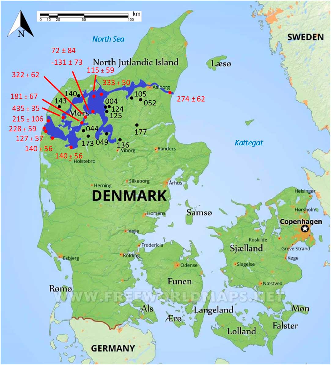
Human and faunal bone material from around the Limfjord was collected from the National Museum in Copenhagen and regional museums in Denmark (Figure 1). The chosen bone samples were not consolidated or visually affected by any form of conservation. The material covers a time span from the Mesolithic (4000 cal BC) up to the Viking Age (1050 cal AD) and was collected as part of a larger project (Stories of Subsistence: people and coast over the last 6000 years in the Limfjord, Denmark), which investigates the interplay between humans and coastal environments.

Figure 1 The Limfjord region, consisting of a series of connected fjords, is highlighted in dark blue in northern Denmark. Samples numbers and their locations used in this study are displayed in black, while the locations and values of ΔR points (Olsson Reference Olsson1980; Heier-Nielsen et al. Reference Heier-Nielsen, Heinemeier, Nielsen and Rud1995) are displayed in red. (Please see electronic version for color figures.)
METHODS
The applied bone collagen extraction protocol (Brock et al. Reference Brock, Higham, Ditchfield and Bronk Ramsey2010) is based on the Longin method (Longin Reference Longin1971) and revised with the inclusion of an ultrafiltration step (Brown et al. Reference Brown, Nelson, Vogel and Southon1988; Bronk Ramsey et al. Reference Bronk Ramsey, Higham, Bowles and Hedges2004). All glassware was baked out at 500°C. Bone samples were mechanically cleaned using a handheld dremel and crushed into smaller pieces, after which 10 mL of 2% (0.6M) hydrochloric (HCl) acid was added to demineralize the bone in 24 hr at room temperature. The acid was renewed to ensure complete demineralization of the sample. After discarding the soluble fraction, samples were rinsed with Milli-Q water three times to neutral pH. Weak HCl acid (pH 3) was added to dissolve the collagen fraction of the sample at ~70˚C for 24 hr, after which samples were filtered using Ezee (Elkay®) filters (60–90 µm) to separate the dissolved collagen fraction from any remaining insoluble particles. The filtered fraction was poured into a thoroughly cleaned ultrafilter with a 30 kDa molecular weight cut-off, which was centrifuged for 20 min at 3000 RPM. The cleaning procedure of the Vivaspin Turbo 15 ultrafilters involved filling with Milli-Q water, centrifuging for 5 min at 3000 rpm to pass the water through the ultrafilter (2 times) followed by one-hour in the ultrasonic bath in Milli-Q water, after which filters were rinsed and filtered again (3 times) following the method of Bronk Ramsey et al. (Reference Bronk Ramsey, Higham, Bowles and Hedges2004). Ultrafiltered samples were transferred into clean vials, frozen using liquid nitrogen and lyophilized.
Isotope Ratio Mass Spectrometry (IRMS)
1–1.5 mg of collagen was weighed into tin capsules and analyzed for carbon and nitrogen stable isotope ratios using the Flash 1112 elemental analyzer coupled to a Thermo Delta V IRMS at the 14CHRONO Centre in Queen’s University Belfast. The collagen samples were run with standards IA-R041 L-Alanine (δ15N –5.56; δ13C –23.33), IAEA-N-2 Ammonium Sulphate (δ15N=+20.3 ± 0.2) and IAEA-CH-Sucrose (δ13C=–10.449 ± 0.033). The standard deviation on the measurements of over 1500 measurements of the IA-R041 L-Alanine (δ15N –5.56; δ13C –23.33) standard yielded standard deviations on δ13C and δ15N of 0.22‰ and 0.15‰, respectively. A test on 10 bone collagen samples extracted from a number of different species found that with the exception of a whale bone sample the variability was less than the IA-R041 standard variability which is reported as the uncertainty of the measurements. For hydrogen stable isotope analysis, subsamples of bone collagen (0.35–0.40 mg) were weighed into silver capsules, crimped into balls and placed within a sealed desiccator containing 10 mL water of known isotopic composition. One subsample was placed into a desiccator containing local snow water collected from the Mourne Mountains, Northern Ireland, with δ2H= –56.89‰, while the other subsample was placed in a desiccator containing water from the standard USGS 49 with δ2H= –394.7‰. Samples were left to equilibrate in the two desiccators for 4 days (96 hr) at ambient temperature. The water was removed and samples were dried down for 7 days under a vacuum in sealed desiccators containing silica gel to remove any water vapor. Due to the lack of a hermetically sealed autosampler during the analysis of the first sample batch, 3 samples were taken from the desiccators every 15 min and placed in the running Thermo MAS 200R autosampler to reduce exposure to ambient air as much as possible (<30 min). The first sample was flushed with helium before being dropped into the reactor and combusted at 1447°C. Substituting the original Thermo autosampler for a Costech Zeroblank autosampler meant that the entire carousel (50 positions) was flushed with 300 mL/min helium for 10 min, after which the autosampler was sealed, protecting samples from the atmosphere. Each autosampler arrangement was coupled to a Thermo high temperature conversion elemental analyzer (TC/EA). The reactor within the TC/EA consisted of an outer ceramic mantle tube of aluminium oxide and an inner glassy carbon reactor part-filled with glassy carbon chips. A graphite crucible sat on these chips and received each dropped sample from the autosampler/Zeroblank arrangement. Each crucible received a maximum of 200 samples before replacement. For isotopic measurement the TC/EA was coupled with a Thermo Delta V IRMS at the Stable Isotope Facility in the School of Planning, Architecture and Civil Engineering of Queen’s University Belfast. To ensure machine integrity, both stability and linearity checks (H3 + correction check for the δ2H measurements) were carried out on the IRMS before each run. Machine precision was 0.4‰. Samples were calibrated using international standards packed in 0.25 μL silver tubes (Qi et al. Reference Qi, Gröning, Coplen, Buck, Mroczkowski, Brand, Geilmann and Gehre2010), VSMOW (δ2H= 0‰), SLAP-2 (δ2H= –427.5‰) and UC04 (δ2H= +113‰). Hydrogen values (%) were measured by comparing the area under its intensity response curve with an Atropina standard of known hydrogen content (8.01%) analyzed by the same method. A run consisted of 12 standards (4 SLAP-2, 4 VSMOW, 4 UC04), 3 Atropina standards, 2 blanks, 22 samples, followed by 1 blank and 9 standards (3 SLAP-2, 3 VSMOW, 3 UC04). The average δ2H values of two duplicate measurements was calibrated against international standards VSMOW, SLAP-2 and UC04.
Accelerator Mass Spectrometry (AMS)
2.5–3 mg of collagen was loaded with 0.09 g of copper oxide and a silver strip for contaminant removal in a small quartz tube for combustion to CO2 at 850°C for 8 hr. Combusted samples were graphitized using a hydrogen reduction method with iron as catalyst. Combustion and graphitization protocols follow standard protocols at the 14CHRONO Centre in Belfast. Pressed targets were analyzed together with oxalic acid standards and background samples in the NEC compact model 0.5MV AMS at the 14CHRONO Centre in Belfast (Reimer et al. Reference Reimer, Hoper, McDonald, Reimer, Svyatko and Thompson2015) including the use of a mammoth bone process blank (background). Radiocarbon ages were calculated from F14C (Reimer et al. Reference Reimer, Baillie, Bard, Bayliss, Beck, Bertrand, Blackwell, Buck, Burr, Cut- ler, Damon, Edwards, Fairbanks, Friedrich, Guilderson, Hogg, Hughen, Kromer, McCormac, Manning, Bronk Ramsey, Reimer, Remmele, Southon, Stuiver, Talamo, Taylor, van der Plicht and Weyhenmeyer2004), which is corrected for background and isotopic fractionation using 13C/12C measured by AMS that accounts for both natural and machine isotopic fractionation. An error multiplier of 1.3 was applied to the F14C measurements to account for variability in sample processing. 14C dates were calibrated using CALIB 7.0.2 with the mixed marine curve for humans (Reimer et al. Reference Reimer, Bard, Bayliss, Warren Beck, Blackwell, Bronk Ramsey, Buck, Cheng, Lawrence Edwards, Friedrich, Grootes, Guilderson, Haflidason, Hajdas, Hatté, Heaton, Hoffmann, Hogg, Hughen, Felix Kaiser, Kromer, Manning, Niu, Reimer, Richards, Marian Scott, Southon, Staff, CSM and van der Plicht2013).
RESULTS AND DISCUSSION
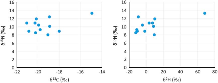
All samples produced acceptable atomic C:N ratios (2.9–3.6) (DeNiro Reference DeNiro1985) and acceptable collagen yields (>0.5–1%) (van Klinken Reference van Klinken1999). Considerable variation in the δ2H values of duplicate measurements (0.1–11.5‰) was observed in the first batch, after which it was decided to homogenize the samples using a small agate mortar and pestle. After the first sample batch, the Costech ZeroBlank autosampler was purchased, enabling a much swifter and more reliable way of measuring δ2H values. However, the reference materials in silver tubes purchased from the USGS were so small that they blocked the autosampler’s carousel. To prevent this from happening, the silver tubes were loaded in loosely crimped silver capsules, although the capsules had to be crimped to a small enough size so not to block the entrance of the combustion tube in the reactor. Duplicate runs generally gave very little variation (<2‰), although some samples still had more variable hydrogen isotope ratios (<5‰), while three samples gave variation >7‰ (7.2‰, 7.7‰, and 10.3‰). This was usually the case for samples with very fluffy white collagen, which was difficult to homogenize. The percentage hydrogen in samples varied between 3.2% and 5.4%. Hydrogen percentages are absent for 5 samples, as the standard was not run in the first batch of samples. Hydrogen stable isotope ratios were measured in 60 samples but only 12 were also radiocarbon dated. These 12 samples are the focus of this paper (Figure 2). The overview of the hydrogen isotope measurements in Table 1 shows the increasing average δ2H values per trophic level, with the herbivores (cattle, sheep) producing the lowest δ2H values, followed by omnivores (pigs, humans), carnivores (dogs), while marine top predators (seal, orca) displayed the highest δ2H values.

Figure 2 Stable isotope plots (δ13C and δ15N, and δ15N and δ2H) from the 12 human individuals.
Table 1 Hydrogen stable isotope results reported in per mil (‰) relative to V-SMOW per species listed by increasing trophic level (from cattle to orca). N refers to the number of specimens and the values from van der Sluis et al. (Reference van der Sluis, Hollund, Kars, Sandvik and Denham2016) are from single sites.
In the current literature there is a lack of studies reporting δ2H values on archaeological human bone collagen samples. Still, existing data from two studies are compared to our results. Reynard and Hedges (Reference Reynard and Hedges2008) used samples originating from various places across Europe which were dated to various archaeological periods (from the Neolithic to the Middle Ages), while material from Norway (van der Sluis et al. Reference van der Sluis, Hollund, Kars, Sandvik and Denham2016) covered a shorter time span (Viking Age to Medieval/early modern times). The increase in δ2H values per trophic level in this study using material from the Limfjord (Table 1) is similar to the results of Reynard and Hedges (Reference Reynard and Hedges2008), who reported certain ranges in the δ2H values of animal species feeding at different trophic levels (Table 2). The Norwegian study showed a large deviation in the step from herbivores to humans. This can most likely be explained by the consumption of considerable amounts of marine fish, which is probably connected to the time periods as well as religious beliefs—marine fish was a common dietary supplement in the Viking Age and especially in early (Catholic) Christian times during periods of fasting. The Limfjord’s dataset covers a large timespan (Mesolithic up to the Viking Age) similar to Reynard and Hedges’ work, and also produced similar δ2H ranges.
Table 2 Comparison of trophic level shifts inferred from δ2H values from the Limfjord region to samples from across Europe (Reynard and Hedges Reference Reynard and Hedges2008) and Stavanger region, Norway (van der Sluis et al. Reference van der Sluis, Hollund, Kars, Sandvik and Denham2016). The Reynard and Hedges (Reference Reynard and Hedges2008) δ2H trophic shifts are a range from 5 sites whereas this study and the van der Sluis et al. (Reference van der Sluis, Hollund, Kars, Sandvik and Denham2016) values are from single sites.

Using δ2H, δ13C and δ15N Values to Estimate Marine Dietary Intake
Consumption of marine resources can result in an apparent older 14C age in the consumer, which can be reservoir corrected using a ΔR value and an estimate of the amount of dietary marine intake, which is ordinarily done using δ13C values and occasionally done using δ15N values (Fischer et al. Reference Fischer, Olsen, Richards, Heinemeijer, Sveinbjörnsdóttir and Bennike2007). In this study, three stable isotope ratios (δ2H, δ13C, and δ15N) are used to estimate the proportion of marine protein in the diet. There are 12 samples of which the 14C ages, δ2H, δ13C, and δ15N values are available in Table 3, which is ordered chronologically based on the uncalibrated 14C ages. The percentage of marine food intake was calculated based on linear interpolation between a terrestrial and marine endpoint: –21.5‰ and –11.8‰ were used for δ13C values, 5.4‰ and 13.1‰ for δ15N values and –47.0‰ and 87.0‰ for δ2H values. The δ13C and δ15N values of the terrestrial endmembers are based on the average of stable isotope results from 53 herbivore bone samples from the Limfjord area, while the marine endmember values based on the average of stable isotope results from 27 bone samples from marine animals (van der Sluis Reference van der Sluis2017). Hydrogen stable isotope analysis was executed on a selection of bone samples, 13 herbivores and 10 marine animals (fish, seal and orca) (Table 1). A diet to consumer offset of 1‰ was applied to the δ13C values (DeNiro and Epstein Reference DeNiro and Epstein1978), 3‰ to the δ15N values (DeNiro and Epstein Reference DeNiro and Epstein1981) and 30‰ to the δ2H values. Calibrated ages are calculated in Calib 7.0.2 based on mixed IntCal13 and Marine13 calibration curves (Reimer et al. Reference Reimer, Bard, Bayliss, Warren Beck, Blackwell, Bronk Ramsey, Buck, Cheng, Lawrence Edwards, Friedrich, Grootes, Guilderson, Haflidason, Hajdas, Hatté, Heaton, Hoffmann, Hogg, Hughen, Felix Kaiser, Kromer, Manning, Niu, Reimer, Richards, Marian Scott, Southon, Staff, CSM and van der Plicht2013) using a ΔR=239 and σ=164 based on 13 14C measurements of known aged marine molluscs from the Limfjord region (Olsson Reference Olsson1980; Heier-Nielsen et al. Reference Heier-Nielsen, Heinemeier, Nielsen and Rud1995) and taken from the online marine database (http://calib.org/marine/). The δ13C and δ2H values are moderately correlated (R2=0.55 p=1×10⁻⁶), while the δ15N and δ2H values are poorly correlated (R2=0.29 p=2×10⁻³). Using δ15N values to estimate the amount of marine protein intake generally results in higher percentages, especially in younger samples, which could be due to intensive fertilization practices in younger periods. This can be solved by applying a higher (for example 4‰) diet to consumer offset, although this would result in negative numbers in the estimated amount of marine intake in older samples.
Table 3 Uncalibrated radiocarbon ages and calibrated 14C ages using δ13C, δ15N and δ2H value to quantify marine carbon (%M). Negative values of %M are shaded in gray. Period and period changes separated by “/” indicate the calibrated age range is on the boundary between two archaeological periods.
* Archaeological period based on calibration of the 14C ages using δ13C values to estimate the marine protein intake.
** Change in archaeological period using δ15N values compared with the calibration of the 14C ages using δ13C values to estimate the marine protein intake.
*** Change in archaeological period using δ2H values compared with the calibration of the 14C ages using δ13C values to estimate the marine protein intake.
The calculated amounts of marine intake differ between the usage of the δ2H, δ13C, and δ15N isotope values (Figure 3) with a maximum difference of 42.1% between the use of δ15N and δ13C, 23.8% between δ2H and δ13C, and 46.2% between δ2H and δ15N. In some cases this results in different archaeological periods (Table 3), although this is often because one of the calibrated ages falls 5–20 years in the preceding or following period. The archaeological periods are given in the column called Period (Table 3), based on calibration of the 14C ages using δ13C values to estimate the marine protein intake. The two columns after the calibrated 14C ages using δ15N and δ2H values are either empty, indicating no difference from the calibrated 14C age using δ13C value, or display the difference in archaeological period. There is still a lot of overlap in the calibrated ages. The difference in calibrated 14C ages using the three different isotope values to estimate the percent marine protein intake is also depicted in Figure 3. Acronyms are used in Table 3 but an overview of the Danish archaeological periods is given in Figure 4. Because younger archaeological periods are often much shorter than older periods, there are more changes in period in the younger samples at the bottom of the table. Perhaps the most advantageous outcome is the lack of negative numbers in the estimated amount of marine protein in the diet using δ2H values (shaded in gray in Table 3). Another potential advantage could be the reduced susceptibility of δ2H values to the manuring effect. Kanstrup et al. (Reference Kanstrup, Thomsen, Andersen, Bogaard and Christensen2011, Reference Kanstrup, Holst, Jensen, Thomsen and Christensen2014) observed on average higher δ15N values in Danish cereal grains from the Iron Age than in grains from the Bronze Age and Neolithic, while a similar trend is not immediately visible in the δ2H values (Table 3). This topic would benefit from studies testing the relationship between manuring and δ2H values.
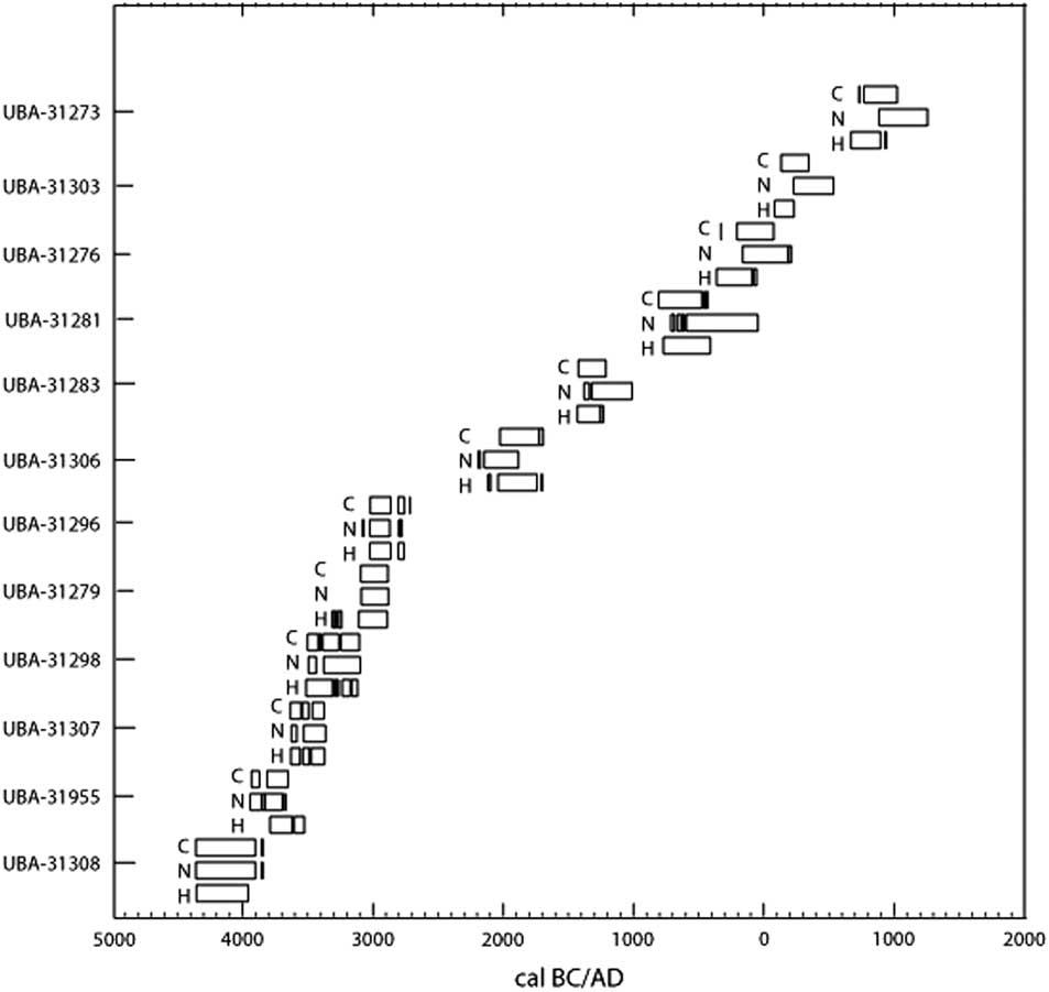
Figure 3 The 2σ calibrated 14C age ranges using δ13C, δ15N, and δ2H values to calculate the percent marine intake, labelled C, N, and H, respectively, from the 12 human individuals. A value of zero was used in place of negative percent marine intake estimates from δ13C and δ15N.
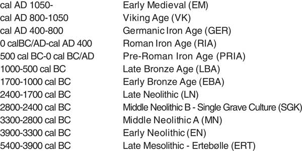
Figure 4 Timetable of Danish prehistoric periods.
CONCLUSION
While we were only able to analyze 12 samples to test if hydrogen stable isotope ratios could be used instead of carbon or nitrogen stable isotope ratios to calculate reservoir offsets, the results seem promising. At the very least the hydrogen isotope ratios circumvented the negative percent marine intakes sometimes estimated with δ13C or δ15N and may have reduced susceptibility to manuring effects. This subject would benefit from more testing in the future and potentially using samples from an area with a smaller ΔR and uncertainty.
ACKNOWLEDGMENTS
Wolfram Meier-Augenstein is thanked for sharing his analytical expertise and giving advice regarding the setup for δ2H measurements. The National Museum in Copenhagen and the regional Museums around the Limfjord (Ålborg, Års, Skive, Mors, Thy, Holstebro and Viborg) are thanked for allowing sampling of the bone material. This research was funded by the Leverhulme Trust (RPG-2012-817). Two anonymous reviewers are thanked for their comments and insights.