INTRODUCTION
The anthropogenic addition to the radiocarbon (14C) inventory has caused immense perturbation to the distribution of naturally produced 14C, but provided a valuable tracer for study of the exchange of carbon between different reservoirs. Since the Nuclear Test-Ban Treaty in 1963, the concentration of bomb-produced 14C in the atmosphere has decreased exponentially through the exchanges with the ocean and the terrestrial/biosphere reservoirs and by dilution with CO2 derived from fossil fuel burning (Levin and Kromer Reference Levin and Kromer2004). The upper ocean has absorbed a large amount of bomb 14C through air–sea exchange such that the average 14C of the global surface ocean peaked in approximately 1973, about 10 years following the atmospheric bomb 14C peak in the mid latitude Pacific Ocean (Druffel and Griffin Reference Druffel and Griffin1995). Since the 1980s, the low- and mid-latitude oceans around ±30° N and S have reached isotopic equilibrium with the decreasing atmospheric 14C level (Caldeira et al. Reference Caldeira, Rau and Duffy1998).
The bomb 14C pulse and subsequent decline have been used to constrain the global mean CO2 exchange velocity and assess the ocean circulation processes that regulate oceanic uptake and storage of anthropogenic CO2 (Broecker et al. Reference Broecker, Peng, Ostlund and Stuiver1985; Toggweiler et al. Reference Toggweiler, Dixon and Bryan1989; Krakauer et al. Reference Krakauer, Randerson, Primeau, Gruber and Menemenlis2006; Sweeney et al. Reference Sweeney, Gloor, Jacobson, Key, McKinley, Sarmiento and Wanninkhof2007; Graven et al. Reference Graven, Gruber, Key, Khatiwala and Giraud2012). In contrast to the high-precision atmospheric bomb 14C records on land (Levin and Kromer Reference Levin and Kromer2004; Turnbull et al. Reference Turnbull, Lehman, Miller, Sparks, Southon and Tans2007; Levin et al. Reference Levin, Kromer and Hammer2013), very limited data have been obtained on maritime air samples over the oceans (Bhushan et al. Reference Bhushan, Krishnaswami and Somayajulu1997; Dutta Reference Dutta2002; Kitagawa et al. Reference Kitagawa, Mukai, Nojiri, Shibata, Kobayashi and Nojiri2004; Dutta et al. Reference Dutta, Bhushan, Somayajulu and Rastogi2006). In a series of air–sea CO2 exchange studies in the Northern Indian Ocean, Bhushan et al. (Reference Bhushan, Krishnaswami and Somayajulu1997) and Dutta et al. (Reference Dutta, Bhushan, Somayajulu and Rastogi2006) measured tropospheric 14C in the maritime air over the Arabian Sea and the Bay of Bengal. They showed that the 14CO2 over this region decreased from 120 ± 3‰ in 1993 to 85±2‰ in 2001. Kitagawa et al. (Reference Kitagawa, Mukai, Nojiri, Shibata, Kobayashi and Nojiri2004) reported tropospheric 14C of a Japan-Australia transect over the western Pacific during 1994–2002 and revealed a similar decreasing trend of maritime air 14CO2 as in the remote background monitoring sites on land during the past decades.
The South China Sea (SCS) is the largest marginal sea in the western Pacific. The region is under strong influence of Asian monsoon, characterized by prevailing northeasterly winds in winter and southwesterly winds in summer. Driven by the seasonally reversed monsoon winds, the general circulation in the SCS upper layer is cyclonic in winter and anticyclonic in summer, respectively (Wyrtki Reference Wyrtki1961; Shaw and Chao Reference Shaw and Chao1994; Qu Reference Qu2000a; Su Reference Su2004; Gan et al. Reference Gan, Li, Curchitser and Haidvogel2006; Fang et al. Reference Fang, Wang, Wei, Fang, Qiao and Hu2009). Intrusions of Kuroshio Current through the Luzon Strait and mesoscale variability induced by eddies are also important features in the northeastern SCS (Qu et al. Reference Qu, Mitsudera and Yamagata2000b; Centurioni et al. Reference Centurioni, Niiler and Lee2004; Nan et al. Reference Nan, Xue and Yu2015), which add complexity for the surface water circulation as well as for the oceanic exchange with atmosphere. Several studies have been conducted to assess the sea–air CO2 fluxes in the SCS and shown that most areas of the SCS served as weak to moderate sources of CO2 to the atmosphere (Dai et al. Reference Dai, Cao, Guo, Zhai, Liu, Yin, Xu, Gan, Hu and Du2013; Zhai et al. Reference Zhai, Dai, Chen, Guo, Li, Shang, Zhang, Cai and Wang2013). However, no records of maritime air 14CO2 and sea surface water DI14C have been documented in the SCS. There were only four middle-deep depth (420–4170 m) seawater DI14C data measured by Broecker et al. (Reference Broecker, Patzert, Toggweiler and Stuiver1986) at one station in the central SCS. In this study, we measured 14C in CO2 of the maritime air collected over the SCS and 14C of the DIC in the sea surface water (∼5 m depth) in the same region. It is hoped that these measurements could have potentially important implications on the estimate of the air-sea CO2 exchange and ocean circulation processes in this region.
MATERIAL AND METHODS
Air and Seawater Sampling
Maritime air and surface seawater samples were collected onboard the R/V Dongfanghong 2 during a scientific investigation cruise in 2014, as part of the South China Sea Deep Processes project of the National Natural Science Foundation of China.
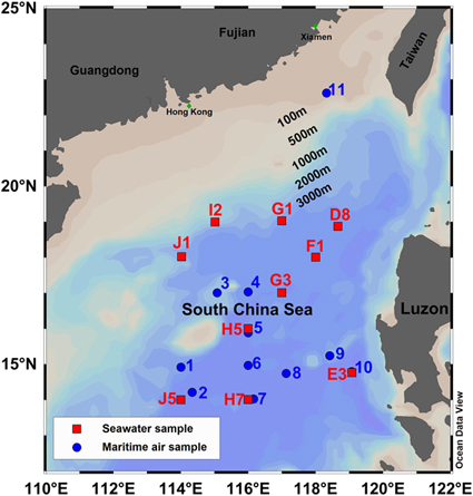
Ten maritime air samples were collected in the SCS open ocean area (>100 km from the shore) on July 6-15, 2014, and the last one was collected on the northeastern continental shelf of the SCS (∼200 km from Xiamen) by the third leg of the cruise on July 6–17, 2014. The sampling sites are plotted in Figure 1 and the weather conditions for each sample are listed in Table 1. About 3.3 L of maritime air was sucked directly into a pre-evacuated stainless steel canister for about 1 min until it reached atmospheric pressure. The sampling location was located on the top deck of the vessel (about 10 m above sea level). In order to avoid any contamination from ship exhaust, air samples were collected during cruising after it left the seawater sampling site. Thus, the air and seawater sampling sites were not completely overlapping, but coupled in the best way feasible. Wind speed (m/s) and wind direction (meteorological convention, 0º = wind comes from the north) were obtained from the shipboard meteorological instrument.

Figure 1 Sampling sites for maritime air and sea surface water in the SCS during the cruise in 2014. The letters of the seawater samples were names of different sections (from A to J) which followed the experimental design of the cruise in 2014; while the air samples stations were simply named after their sampling sequence.
Table 1 Sampling information and 14C results of the SCS atmospheric CO2. The 14C uncertainties are the analytical errors from individual measurements.

During the 2nd and 3rd legs of the cruise between June 20 and July 14, 10 surface seawater samples were collected with the Carousel Water Sampler attached on a SBE 917 plus CTD (conductivity-temperature-depth; Sea-Bird Electronics Inc). Seawater samples of about 100 mL were collected at a depth of 5 m at each station and poisoned with 50 μL of saturated HgCl2 solution immediately. The seawater sampling sites and their detailed sampling information are given in Table 2 and plotted in Figure 1. Seawater temperature (ºC) and salinity (psu) values were derived using the software package SBE Data Processing-Win32.
Table 2 Sampling information and 14C results of the SCS surface water DIC. The 14C uncertainties are the analytical errors from individual measurements.

14C Analysis
Both air and seawater samples were processed for 14C analysis at the Cosmogenic Nuclide Sample Preparation Laboratory of the Key Laboratory for Earth Surface Processes in Peking University, China. Atmospheric CO2 was cryogenically purified on a vacuum line and then graphitized with the sealed-tube Zn reduction method (Xu et al. Reference Xu, Trumbore, Zheng, Southon, McDuffe, Luttgen and Liu2007). DIC from seawater samples was extracted using the headspace-extraction method (Gao et al. Reference Gao, Xu, Zhou, Pack, Griffin, Santos, Southon and Liu2014) from a volume of 30 mL after acidification with H3PO4, and then purified and graphitized in the same way as the CO2 samples. Graphite samples were pressed into aluminum targets and measured for 14C at Peking University Accelerator Mass Spectrometry (PKUAMS) facility (Liu et al. Reference Liu, Ding, Fu, Pan, Wu, Guo and Zhou2007).
All 14C results discussed in the text are expressed as the per mil deviation (Δ14C) from 95% of the NBS oxalic acid I (OX-I) activity in 1950 as defined by Reimer et al. (Reference Reimer, Thomas and Reimer2004) (with the age correction back to the sampling year), and are fractionation corrected to –25‰ using the online 13C/12C measurements in the AMS system which account for all potential fractionations occurred during the laboratory procedures and AMS measurements. For future reference, the 14C results are also presented as fraction modern (F14C) in Tables 1 and 2. The precision of Δ14C measurements for modern samples is ∼3‰ based on long-term measurements of secondary standards, such as OX-II, IAEA-C6, IAEA-C2, and CSTD-Coral. The 14C uncertainties reported in this study are mainly the counting statistical errors from individual AMS measurements but adjusted based on the precisions of the six OX-I standards measured in the same wheel.
RESULTS
14CO2 over the SCS
The Δ14C values of 11 individual maritime air samples are listed in Table 1 and plotted in Figure 2 (left). The average Δ14C of the central SCS maritime air was 19.0±2.4‰ (1 σ stdev, n = 10), with a range from 15.6±1.6‰ to 22.0±1.6‰. Samples collected from sites close to one another on the same day (e.g., Stations 3 and 4, 5 and 6, 7 and 8) yielded Δ14C values in excellent agreement with each other (17.0 ± 1.5‰ and 20.3±1.6‰; 15.6±1.6‰ and 16.3±1.5‰; 18.6±1.5‰ and 22.0±1.6‰), indicating that the sampling procedure and measurements were robust. Station 11, located next to the continental margin of Southeastern China, showed a much depleted Δ14C value of 8.3±1.5‰, which was ∼10‰ lower than the central SCS maritime air Δ14C values.

Figure 2 Δ14C distributions of maritime air CO2 (left) and surface seawater DIC (right) of the SCS.
DI14C of Surface Seawater in the SCS
The Δ14C values of 10 individual surface seawater samples are listed in Table 2 and plotted in Figure 2 (right). They varied between 28.3 ± 2.5‰ and 40.6 ± 2.7‰, with an average of 34.4 ± 4.5‰ (1 σ stdev, n = 10). Stations E3 and D8, which are located in the easternmost part of the sampling area, displayed the highest Δ14C values of about 40‰ among all stations. The lowest Δ14C values (29.9‰ and 28.3‰ at Stations H5 and H7, respectively) were observed in the central SCS along the 116˚E section. Mid-range Δ14C values of 31.5‰ and 34.6‰ were observed at stations J5 and J1, respectively, in the western part of the study area.
DISCUSSION
Δ14C Spatial Variations and their Controls
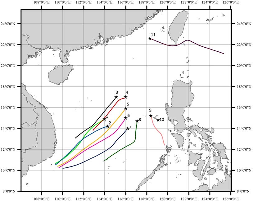
The temporary wind direction varied between 171º and 295º and the wind speed was between 3.4 and 7.6 m/s at the time of maritime air sampling in the central SCS (excluding Station 11), indicating that the area was mainly influenced by strong southwest wind during the period of July 6–15, 2014. In order to show the air mass source and transport route for a longer time, backward trajectory plot (Figure 3) derived from the NOAA HYSPLIT model (Draxler and Rolph Reference Draxler and Rolph2013) was conducted for the last 24 hr for each sampling site. Air masses arriving Stations 1–8 were basically originated from the southwestern open ocean area and underwent long distance transport. For Station 9, the air mass source shifted to the south and the transport route was relatively short; while Station 10 seemed to be influenced by local air mass since the transport route was confined in a very small area. The results of the back trajectory analysis revealed that most of the central SCS were dominated by air mass from the southwest.

Figure 3 Twenty-four hours air mass back trajectories at 10 m above sea level of the 11 maritime air sampling sites, derived from the NOAA HYSPLIT (Hybrid Single-Particle Lagrangian Integrated Trajectory) Model (http://ready.arl.noaa.gov/HYSPLIT.php).
The Δ14CO2 spatial variation range was ∼6‰ (comparable to the measurement uncertainty) and the average Δ14C value was 19.0 ± 2.4‰ (n = 10) for Stations 1–10, indicating that the maritime air mass in central SCS was very well mixed. The SCS Δ14CO2 value was also in excellent agreement with the atmospheric Δ14CO2 recorded in Barrow, AK, which were 19.1 ± 2.3‰ (n = 6) in June and 21.1 ± 1.7‰ (n = 3) in July 2014 (X. Xu, unpublished data). Such a consistency between the SCS oceanic sites and the Alaskan coastal site points to a well-mixed and clean open ocean air background of 14CO2 at the SCS.
The sample from Station 11, located on the northeastern continental shelf of the SCS (∼200 km away from Xiamen; water depth <50 m), showed a depleted Δ14C value compared to the rest of the maritime air samples. The wind direction shifted to the east (72º) and the wind speed was particularly strong (8.1 m/s) during sampling. The backward air mass trajectories (Figure 3) also suggest that this station was influenced by air mass originated from the east. The differences in wind direction and source regions at this station likely explain the Δ14C depletion, indicating that air masses from the east experienced a dilution of anthropogenic 14C-free CO2 from the fossil fuel emission when passing over Taiwan. A rough calculation based on a simple two-end member mixing suggests that the fraction of fossil fuel CO2 would be ∼1% at Station 11, assuming fossil fuel CO2 with Δ14C of –995‰ and the clean maritime CO2 with a Δ14C of ∼19‰.
During June–July 2014, surface seawater samples collected in the central SCS (Stations H5 and H7) showed the lowest Δ14C values among all the stations. From 116º to 120ºE, surface seawater Δ14C increased along the longitude and showed the highest values in the easternmost stations next to Luzon. The Δ14C spatial variation range of the SCS surface seawater was ∼12‰, which was larger than that of the maritime air in the same region. Besides air–sea exchange processes, other mechanisms such as vertical mixing between surface and subsurface water and/or lateral exchange between different water masses might also be responsible for the observed Δ14C spatial difference.
Since the bomb 14C perturbation has been several decades old and the air–sea gradients in 14C have become substantially smaller, Graven et al. (Reference Graven, Gruber, Key, Khatiwala and Giraud2012) proposed that the changes in global upper layer oceanic 14C are now primarily controlled by shallow-to-deep water (or surface to subsurface) exchange. Inside the SCS basin, vertical mixing induced by physical oceanographic processes such as eddies and internal waves are relatively strong in the Luzon Strait and the continental shelves but relatively weak in the central SCS (Tian et al. Reference Tian, Yang and Zhao2009; Zhang et al. Reference Zhang, Tian, Qiu, Zhao, Chang, Wu and Wan2016). If the surface to subsurface water exchange induced by vertical mixing were the dominant control, the surface water of Luzon Strait and the continental shelves of the SCS would display more depleted Δ14C values compared to those of the central SCS. However, the most depleted surface water Δ14C values were recorded in the central SCS. Hence vertical mixing cannot explain the surface water Δ14C spatial difference observed in the SCS. Other mechanism(s) must be considered.
Compared to the open ocean condition in the western Pacific, the surface water of the SCS is very well mixed with the subsurface water due to overall enhanced vertical mixing in this marginal sea (Tian et al. Reference Tian, Yang and Zhao2009). The surface water Δ14C was 28.3–40.6‰ for the SCS and nearly constant for most of the stations in the upper 150 m (L. Zhou and P. Gao, unpublished data). Furthermore, the surface water of the western Pacific collected in the east of Luzon Strait along the 123ºE transect (sampled on May 27–29, 2014, during the same cruise) had higher Δ14C (39.1–43.6‰) because it did not mix readily with the subsurface waters, and there was usually a subsurface Δ14C maximum (46.4–55.6‰) at depths of around 200 m (L. Zhou and P. Gao, unpublished data). Thus, we attribute the spatial difference in the SCS observed here to the horizontal exchange between the SCS and the western Pacific. Stations in the easternmost part of the sampling area were influenced by the high Δ14C surface water masses from the western Pacific surface waters, probably through the invasion of Kuroshio Current. Although there are some seasonal and inter-annual variations, the horizontal intrusion of western Pacific water through Luzon Strait makes important contribution to the water properties in the upper layer and regulates the surface circulation patterns in the northeastern SCS (Qu Reference Qu2002; Li and Qu Reference Li and Qu2006; Tian et al. Reference Tian, Yang, Liang, Xie, Hu, Wang and Qu2006; Yang et al. Reference Yang, Tian and Zhao2010; Hsin et al. Reference Hsin, Wu and Chao2012; Nan et al. Reference Nan, Xue and Yu2015). In our sampling season, the surface circulation driven by the southwest wind was mainly anti-cyclonic, which would have prevented further invasion of the high Δ14C western Pacific surface waters to the stations west of 118ºE.
Δ14C Difference between Air and Surface Seawater and Its Implications
The measured Δ14C values of the maritime air over the SCS were compared with that of the sea surface water in Figure 4. The average sea surface water DI14C value was 15.4 ± 5.1‰ higher than that of the 14CO2 of central SCS maritime air (excluding Station 11). This was due to both the addition of the 14C-free fossil fuel emission to the atmosphere and the increased bomb 14C accumulation in surface ocean during the past decades (Suess Reference Suess1955; Graven et al. Reference Graven, Gruber, Key, Khatiwala and Giraud2012).

Figure 4 Δ14C difference between the SCS maritime air CO2 (red triangle) and sea surface water DIC (blue circles). Red and blue dashed lines denote the average Δ14C values of maritime air CO2 (excluding Station 11) and sea surface water DIC, respectively.
The 14C in the air–sea interface is particularly useful for extrapolating CO2 gas exchange parameterizations (Toggweiler et al. Reference Toggweiler, Dixon and Bryan1989; Krakauer et al. Reference Krakauer, Randerson, Primeau, Gruber and Menemenlis2006; Sweeney et al. Reference Sweeney, Gloor, Jacobson, Key, McKinley, Sarmiento and Wanninkhof2007). Several investigations have been conducted to derive the sea–air CO2 fluxes in the SCS (Dai et al. Reference Dai, Cao, Guo, Zhai, Liu, Yin, Xu, Gan, Hu and Du2013; Zhai et al. Reference Zhai, Dai, Chen, Guo, Li, Shang, Zhang, Cai and Wang2013). The Δ14C in the SCS maritime air and surface seawater can help further constrain the air–sea exchange rate and assess the potential ability of the SCS as a natural and anthropogenic CO2 source or sink.
Overall, the low latitude coastal systems outgas CO2 due to the high temperature, high pCO2 and high terrestrial organic carbon (OC) input. Dai et al. (Reference Dai, Cao, Guo, Zhai, Liu, Yin, Xu, Gan, Hu and Du2013) and Zhai et al. (Reference Zhai, Dai, Chen, Guo, Li, Shang, Zhang, Cai and Wang2013) showed that most areas of the SCS served as weak to moderate sources of the atmospheric CO2, and in summer the source term was more significant than that in other seasons. In our sampling season, the surface ocean of the SCS would be expected to act as a CO2 source, outgassing high 14C to the atmosphere and causing some increase of maritime air 14C in the region. However, there were seasonal changes and even reversal from source to sink in the SCS in regions such as the area off the Pearl River estuary (Zhai et al. Reference Zhai, Dai, Chen, Guo, Li, Shang, Zhang, Cai and Wang2013). In such areas, the surface ocean might become a CO2 sink, and the absorption of 14C-depleted maritime air CO2 could induce the lower 14C into the surface water layer.
Nevertheless, as a marginal sea, the SCS has very active upper layer vertical mixing; coastal upwelling might bring water to the surface and liberate CO2 to the atmosphere. The Δ14C of the upwelling water depends on the depth of the water source; upwelled subsurface water has the similar high Δ14C values as the surface water, while upwelled deep water with depleted Δ14C will cause a decrease in surface water Δ14C. Such processes may have a positive or negative effect on the maritime air 14CO2 through air–sea exchange processes.
Temporal Trends of the Air and Surface Seawater Δ14C
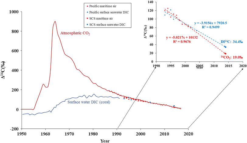
By comparing to the historical data, Figure 5 illustrates the temporal change in atmospheric 14CO2 and surface seawater DI14C since 1950. During the period of pre-1957, 14C of atmospheric CO2 stayed close to 0‰ (natural atmospheric 14C level at the time). As the equilibration timescale (∼10 yr; Broecker and Peng Reference Broecker and Peng1974) of 14C/12C ratio between the surface ocean and the CO2 in the overlying air is longer than the residence time of water in the surface mixed layer, the 14C level of DIC in the surface ocean is far from equilibrium with the atmosphere. Measurements of coral carbonate pre-1957 showed that surface water DIC averaged around −50‰ (Druffel and Suess Reference Druffel and Suess1983), which gave a mean marine surface reservoir age of ∼400 yrs. After the thermonuclear weapons testing, the 14C content of tropospheric CO2 peaked to a level of ∼840‰ in the Northern Hemisphere by 1964, and then decreased quasi-exponentially in the following decades to about 31.5 ± 2.0‰ in 2012 (Levin et al. Reference Levin, Kromer and Hammer2013). Before the 1990s, the decline of the tropospheric 14CO2 was mainly caused by the exchange of bomb 14C with the stratosphere and with the ocean and the terrestrial biosphere, but subsequently was increasingly controlled by the input of 14C-free fossil fuel derived CO2 (Levin et al. Reference Levin, Naegler, Kromer, Diehl, Francey, Gomez-Pelaez, Steele, Wagenbach, Weller and Worthy2010). The bomb 14C entered the ocean and the surface water DI14C increased to about 130‰ by 1974 (Druffel and Griffin Reference Druffel and Griffin1995), while the sea–air Δ14C gradients reached a value of around –300‰ at the same time. As the bomb 14C inventory had built up continuously in the upper ocean, the sea–air Δ14C gradients decreased to the pre-bomb level of –50‰ in the late 1980s and became substantially smaller in 1990s (Figure 5). The western Pacific maritime air 14CO2 (Kitagawa et al. Reference Kitagawa, Mukai, Nojiri, Shibata, Kobayashi and Nojiri2004) and surface water DI14C (Key et al. Reference Key, Kozyr, Sabine, Lee, Wanninkhof, Bullister, Feely, Millero, Mordy and Peng2004) had approached about the same value in the late 1990s. By 2014, the modern sea–air Δ14C gradient in the SCS showed a positive value of 15.4‰ (Figures 4 and 5), the upper ocean has now becoming a source of bomb 14C and is capable of transferring 14C back to the atmosphere.

Figure 5 Decreasing trend of bomb 14C in the air of the mid-latitudes in the Northern Hemisphere (red curve, Levin and Kromer Reference Levin and Kromer2004; Levin et al. Reference Levin, Kromer and Hammer2013; Hammer and Levin Reference Hammer and Levin2017) and in surface water DIC derived from corals around 23ºS in the Pacific Ocean (blue curve, Druffel and Suess Reference Druffel and Suess1983; Druffel and Griffin Reference Druffel and Griffin1995). Annual averaged Δ14C values of Pacific maritime air CO2 between 17ºS–28ºN from Kitagawa et al. (Reference Kitagawa, Mukai, Nojiri, Shibata, Kobayashi and Nojiri2004) and surface water DI14C data between 0–35ºN and 130–150ºE from GLODAP database (Key et al. Reference Key, Kozyr, Sabine, Lee, Wanninkhof, Bullister, Feely, Millero, Mordy and Peng2004) are marked as red and blue triangles, respectively; SCS maritime air 14CO2 and sea surface water DI14C from this study are marked with red and blue circles.
The red and blue dashed line in Figure 5 represent the linear regression trends of maritime air 14CO2 and surface seawater DI14C from the 1990s, respectively. Comparing to the historical data from western Pacific, an average Δ14C decline rate of 5.0‰ per year from 1994 to 2014 was obtained for maritime air, which was compatible to the global trend since the SCS air samples have the same 14CO2 as the continental background station in Alaska. For surface seawater DI14C, a decreasing rate of 3.9‰ per year from 1993 to 2014 was obtained at 14–17ºN in the SCS. This rate may be slightly higher than the global trend, as the SCS has relatively lower surface seawater DI14C compared to the open ocean of western Pacific. The maritime air 14CO2 has decreased faster than the surface seawater DI14C, mainly due to the large size of oceanic carbon reservoir and the dilution of 14C free CO2 from fossil fuel emission to the atmosphere in the past decades. The crossover of the two Δ14C decline trend lines pointed to a reversal from negative to positive sea–air Δ14C gradient at around 2000 in this region (Figure 5).
In the past decades, human-induced bomb 14C has served as an useful tracer to study the carbon exchange between different reservoirs. However, it also introduces ambiguity for conventional radiocarbon dating since at least two samples have to be measured to determine whether the sample was on the increasing or declining side of the bomb curve. The reversal of sea–air Δ14C gradient from negative to positive will add more complication to the reservoir age/residence time of surface water because the gradient is highly depended on the locality of ocean regime, even in the pre-bomb period (Alves et al. Reference Alves, Macario, Ascough and Bronk Ramsey2018). In the following decades when F14C of atmospheric CO2 decreases to less than 1, prior and post bomb samples will no longer be distinguishable by radiocarbon measurement alone. Other proxies such as stable carbon isotope have to be measured for assistance (Köhler Reference Köhler2016). The Δ14C features of global/local carbon reservoirs will change substantially because of the continuous fossil fuel emissions and the release of accumulated bomb 14C in the upper oceans, not only in the mid ocean gyres, but also in some marginal seas such as the SCS that are weak to moderate CO2 sources. More observations should be made on the spatial and temporal variation of sea–air Δ14C gradient, as air–sea gas exchange is not a uniform process over the global oceans, but highly dependent on the local ocean dynamics.
CONCLUSIONS
In this study, we obtained the first records of 14C in the air and surface seawater over the SCS, covering the latitudes of 14–17ºN and longitudes of 114–119ºE. The Δ14C values of the atmospheric CO2 and the seawater DIC varied in the ranges of 15.6 ± 1.6‰ to 22.0 ± 1.6‰ and 28.3 ± 2.5‰ to 40.6 ± 2.7‰, respectively. The Δ14C signature of the maritime air in the SCS was consistent with the clean background air in the Northern Hemisphere except for one station on the northeastern continental shelf of the SCS where noticeable fossil fuel CO2 contribution was observed. There was an eastward increase in 14C value of the seawater DIC, which we attributed to the lateral seawater exchange between the SCS and western Pacific. The sea–air Δ14C gradient in the SCS reached 15.4 ± 5.1‰ in 2014; higher bomb 14C was documented in the surface ocean of this region, thus indicating the possibility of a bomb 14C transfer from the ocean back to the atmosphere. By comparing the present SCS with the 1990s data from the Pacific, decline rates of 5.0‰ and 3.9‰ per year were obtained for maritime air 14CO2 and surface seawater DI14C respectively in this region. It is hoped that more paired measurements of 14C for surface seawater and the air above, together with other seawater DIC concentration/pCO2 data, will serve as a useful tool for constraining the air–sea exchange processes as well as ocean circulation processes in the SCS.
ACKNOWLEDGMENTS
This study was funded by the National Natural Science Foundation of China (No. 91228209) and China Postdoctoral Science Foundation (No. 2015M570889), as well as the 111 Project (B14001). We thank the captain and crew of the R/V Dongfanghong 2 for their assistance and Prof. Shao Min and Lu Sihua for providing the air sampling canisters. We also thank Dr. Zhang Jingcan, Shuai Geiwei, and Huang Tianyi for their help during the onboard sampling, and Qin Xiaoxin for advice on the use of the NOAA HYSPLIT model.