INTRODUCTION
Radiocarbon (14C) is commonly used to date biogenic samples sourcing from over the past 50,000 yr. While alive, organisms equilibrate their 14C/12C ratio with that of the atmospheric pool and, when they die, this ratio begins to decrease as 14C decays. The 14C/12C ratio of a biological sample correlates with the time that has elapsed since its death (Libby Reference Libby1954). However, the atmospheric 14C/12C ratio varies through time and space due to fluctuations of 14C production rate (originating mainly via changes in solar activity and/or in geomagnetic field intensity) and to changes in the carbon cycle, making it necessary to correct atmospheric 14C fluctuations in order to calculate accurate ages. For this purpose, a calibration curve is needed, obtained by comparing raw 14C ages with true calendar ages derived from independent dating methods (e.g. Reimer et al. Reference Reimer, Bard, Bayliss, Beck, Blackwell, Bronk Ramsey, Buck, Cheng, Edwards, Friedrich, Grootes, Guilderson, Haflidason, Hajdas, Hatté, Heaton, Hoffmann, Hogg, Hughen, Kaiser, Kromer, Manning, Niu, Reimer, Richards, Scott, Southon, Staff, Turney and van der Plicht2013).
Various archives are used to construct the 14C calibration curve, but the best is based on dendrochronologically dated tree-ring series. For the Holocene (≈ the past 11,600 yr), subfossil trees are abundant, allowing the construction of a calibration curve dated absolutely with annual resolution. For times before the Holocene, the availability of trees is limited to some areas and periods (Kaiser et al. Reference Kaiser, Friedrich, Miramont, Kromer, Sgier, Schaub, Boeren, Remmele, Talamo, Guibal and Sivan2012). While subfossil trees that lived during warm periods (e.g. Bølling and Allerød phases) are fairly common (Miramont et al. Reference Miramont, Guibal, Kaiser, Kromer, Sgier, Sivan, Friedrich and Talamo2010; Kaiser et al. Reference Kaiser, Friedrich, Miramont, Kromer, Sgier, Schaub, Boeren, Remmele, Talamo, Guibal and Sivan2012; Adolphi et al. Reference Adolphi, Muscheler, Friedrich, Güttler, Wacker, Talamo and Kromer2017; Reinig et al. Reference Reinig, Nievergelt, Esper, Friedrich, Helle, Hellmann, Kromer, Morganti, Pauly, Sookdeo, Tegel, Treydte, Verstege, Wacker and Büntgen2018), trees corresponding to the Younger Dryas cold phase are exceptional (Miramont et al. Reference Miramont, Sivan, Guibal, Kromer, Talamo and Kaiser2011). Indeed, the Younger Dryas (YD) gap prevents the Bølling-Allerød floating sequences from being connected with the absolute chronology (Kaiser et al. Reference Kaiser, Friedrich, Miramont, Kromer, Sgier, Schaub, Boeren, Remmele, Talamo, Guibal and Sivan2012; Reinig et al. Reference Reinig, Nievergelt, Esper, Friedrich, Helle, Hellmann, Kromer, Morganti, Pauly, Sookdeo, Tegel, Treydte, Verstege, Wacker and Büntgen2018).
Capano et al. (Reference Capano, Miramont, Guibal, Kromer, Tuna, Fagault and Bard2018) analyzed 14C in two trees of the Barbiers chronology from the southeast French Alps and reconstructed a continuous 240-yr chronology that was used to tentatively link the absolute calibration curve (Kaiser et al. Reference Kaiser, Friedrich, Miramont, Kromer, Sgier, Schaub, Boeren, Remmele, Talamo, Guibal and Sivan2012) with the floating CELM (Central European Lateglacial Master) chronology for the Allerød period. In this follow-up study, we present an augmented 416-yr tree-ring chronology based on five trees from the Barbiers site, annually 14C dated to the onset of the YD period.
The 14C content measured in French subfossil trees is also compared to kauri records from the Southern Hemisphere (Hogg et al. Reference Hogg, Southon, Turney, Palmer, Bronk Ramsey, Fenwick, Boswijk, Friedrich, Helle, Hughen, Jones, Kromer, Noronha, Reynard, Staff and Wacker2016a, Reference Hogg, Southon, Turney, Palmer, Bronk Ramsey, Fenwick, Boswijk, Buüntgen, Friedrich, Helle, Hughen, Jones, Kromer, Noronha, Reinig, Reynard, Staff and Wacker2016b) and employed to study the atmospheric 14C gradient between the Northern and Southern Hemispheres (NH and SH). Indeed, a systematic 14C difference exists between wood from trees that lived at the exact same time in the NH and SH (SH wood being generally older than NH wood). Precise measurement of this 14C interhemispheric gradient (14C-IHG) and its variations over the Allerød-YD transition is of prime interest for identifying changes in the global carbon cycle during the last deglaciation. The chronological accuracy of the tree-ring record allows comparison of the 14C-IHG variations with other carbon cycle changes evidenced in the atmospheric CO2 and CH4 records measured in bubbles occluded in polar ice cores over the Late Glacial period (Marcott et al. Reference Marcott, Bauska, Buizert, Steig, Rosen, Cuffey, Fudge, Severinghaus, Ahn, Kalk, McConnell, Sowers, Taylor, White and Brook2014).
14C Chronologies from Tree Rings over the Younger Dryas Event
The synchronization of the German HOC (Holocene Oak Chronology) and PPC (Preboreal Pine Chronology) sequences gave rise to a long dendrochronological series, starting (i.e. oldest year) at 12,410 cal. BP (Friedrich et al. Reference Friedrich, Remmele, Kromer, Hofmann, Spurk, Kauser, Orcel and Kuppers2004). This chronology was then extended into the Younger Dryas period with the Swiss YD sequences, leading to an absolute chronology starting at 12,594 cal BP (Schaub et al. Reference Schaub, Kaiser, Frank, Buentgen, Kromer and Talamo2008; Hua et al. Reference Hua, Barbetti, Fink, Kaiser, Friedrich, Kromer, Levchenko, Zoppi, Smith and Bertuch2009, Kaiser et al. Reference Kaiser, Friedrich, Miramont, Kromer, Sgier, Schaub, Boeren, Remmele, Talamo, Guibal and Sivan2012). However, Hogg et al. (Reference Hogg, Turney, Palmer, Southon, Kromer, Bronk Ramsey, Boswijk, Fenwick, Noronha, Staff, Friedrich, Reynard, Guettler, Wacker and Jones2013) highlighted problems in the dendrochronological synchronization of the Ollon505 larch tree with the PPC. Indeed, the 14C data of decadal tree-ring samples from the absolute chronology were included in the IntCal13 calibration curve, but the Ollon505 larch tree was excluded (Reimer et al. Reference Reimer, Bard, Bayliss, Beck, Blackwell, Bronk Ramsey, Buck, Cheng, Edwards, Friedrich, Grootes, Guilderson, Haflidason, Hajdas, Hatté, Heaton, Hoffmann, Hogg, Hughen, Kaiser, Kromer, Manning, Niu, Reimer, Richards, Scott, Southon, Staff, Turney and van der Plicht2013).
In the framework of the 2015 IntCal Workshop in Zurich, Michael Friedrich corrected the matching of sequences and validated the chronology up to 12,325 cal BP (Kromer et al. Reference Kromer, Friedrich and Talamo2015). New dendrochronological and 14C analyses performed in Zurich have been dedicated to filling the gap between the absolute chronology and the YD floating chronologies (Reinig et al. Reference Reinig, Nievergelt, Esper, Friedrich, Helle, Hellmann, Kromer, Morganti, Pauly, Sookdeo, Tegel, Treydte, Verstege, Wacker and Büntgen2018). In addition, floating tree-ring chronologies also exist for the Allerød period: the German LGP (Late Glacial Pine) and the Swiss SWILM (Swiss Late-glacial Master) chronologies, synchronized in the CELM chronology; Italian chronologies from Carmagnola and Avigliana; and French chronologies from the Drouzet site (Kaiser et al. Reference Kaiser, Friedrich, Miramont, Kromer, Sgier, Schaub, Boeren, Remmele, Talamo, Guibal and Sivan2012; Adolphi et al. Reference Adolphi, Muscheler, Friedrich, Güttler, Wacker, Talamo and Kromer2017).
For the YD onset, only a few floating chronologies are available for the NH:
The Barb12-17 sequence, a 240-yr chronology belonging to the French Barbiers chronology that has been sampled at annual resolution for 14C measurements (Capano et al. Reference Capano, Miramont, Guibal, Kromer, Tuna, Fagault and Bard2018). Preliminary 14C dating of the Barb12-17 sequence between ca. 12,836 to 12,594 cal BP (Capano et al. Reference Capano, Miramont, Guibal, Kromer, Tuna, Fagault and Bard2018) was based on visual matching of wiggles against the kauri sequence from New Zealand (Hogg et al. Reference Hogg, Southon, Turney, Palmer, Bronk Ramsey, Fenwick, Boswijk, Friedrich, Helle, Hughen, Jones, Kromer, Noronha, Reynard, Staff and Wacker2016a, Reference Hogg, Southon, Turney, Palmer, Bronk Ramsey, Fenwick, Boswijk, Buüntgen, Friedrich, Helle, Hughen, Jones, Kromer, Noronha, Reinig, Reynard, Staff and Wacker2016b).
The youngest part of the CELM chronology, a 1606-yr chronology composed of Swiss and German pines from the Danube (Kaiser et al. Reference Kaiser, Friedrich, Miramont, Kromer, Sgier, Schaub, Boeren, Remmele, Talamo, Guibal and Sivan2012). The last ring of the youngest tree of the sequence (G5) has been dated in several works to between ca. 12,500 and 12,844 ± 32 cal BP (Hughen et al. Reference Hughen, Southon, Lehman and Overpeck2000; Muscheler et al. Reference Muscheler, Kromer, Björck, Svensson, Friedrich, Kaiser and Southon2008; Hua et al. Reference Hua, Barbetti, Fink, Kaiser, Friedrich, Kromer, Levchenko, Zoppi, Smith and Bertuch2009; Bronk Ramsey et al. Reference Bronk Ramsey, Staff, Bryant, Brock, Kitagawa, van der Plicht, Schlolaut, Marshall, Brauer, Lamb, Payne, Tarasov, Haraguchi, Gotanda, Yonenobu, Yokoyama, Tada and Nakagawa2012; Hogg et al. Reference Hogg, Southon, Turney, Palmer, Bronk Ramsey, Fenwick, Boswijk, Buüntgen, Friedrich, Helle, Hughen, Jones, Kromer, Noronha, Reinig, Reynard, Staff and Wacker2016b; Capano et al. Reference Capano, Miramont, Guibal, Kromer, Tuna, Fagault and Bard2018).
The Swiss YD chronologies. YDB (Younger Dryas B) was the oldest series included in the absolute dendrochronological sequence starting at 12,594 cal BP (Schaub et al. Reference Schaub, Kaiser, Frank, Buentgen, Kromer and Talamo2008). The 14C measurements have been complemented with measurements at annual resolution of the original YD series and of the new floating Late Glacial subfossil pine chronologies from Zurich, Switzerland, the so-called “Binz” find (Reinig et al. Reference Reinig, Nievergelt, Esper, Friedrich, Helle, Hellmann, Kromer, Morganti, Pauly, Sookdeo, Tegel, Treydte, Verstege, Wacker and Büntgen2018; Sookdeo et al. Reference Sookdeo, Wacker, Adolphi, Beer, Büntgen, Friedrich, Helle, Hogg, Kromer, Muscheler, Nievergelt, Palmer, Pauly, Reinig, Turney and Synal2019).
For the SH, the YD period is recorded in two floating chronologies. As is the case for NH records, these chronologies have been dated through 14C measurements:
The huon pine [Lagarostrobos franklinii (Hook.f.) Quinn] chronology from Tasmania (Australia), a floating 617-yr chronology dated through wiggle-matching to ca. 12,760–12,070 cal BP (Hua et al. Reference Hua, Barbetti, Fink, Kaiser, Friedrich, Kromer, Levchenko, Zoppi, Smith and Bertuch2009). The LGP chronology reaching ca. 14,200 cal BP, was linked to the absolute chronology by using the huon pine bridge (Reimer et al. Reference Reimer, Bard, Bayliss, Beck, Blackwell, Bronk Ramsey, Buck, Cheng, Edwards, Friedrich, Grootes, Guilderson, Haflidason, Hajdas, Hatté, Heaton, Hoffmann, Hogg, Hughen, Kaiser, Kromer, Manning, Niu, Reimer, Richards, Scott, Southon, Staff, Turney and van der Plicht2013).
The kauri [Agathis australis (D. Don) Steudel] chronology, a 1451-yr floating chronology from Towai (New Zealand), which spans the period between ca. 13,134 and 11,694 cal BP based on the 14C wiggle-matching with the absolute IntCal13 curve overlapping between 11,874 and 11,694 cal BP (Hogg et al. Reference Hogg, Southon, Turney, Palmer, Bronk Ramsey, Fenwick, Boswijk, Friedrich, Helle, Hughen, Jones, Kromer, Noronha, Reynard, Staff and Wacker2016a, Reference Hogg, Southon, Turney, Palmer, Bronk Ramsey, Fenwick, Boswijk, Buüntgen, Friedrich, Helle, Hughen, Jones, Kromer, Noronha, Reinig, Reynard, Staff and Wacker2016b; Reimer et al. Reference Reimer, Bard, Bayliss, Beck, Blackwell, Bronk Ramsey, Buck, Cheng, Edwards, Friedrich, Grootes, Guilderson, Haflidason, Hajdas, Hatté, Heaton, Hoffmann, Hogg, Hughen, Kaiser, Kromer, Manning, Niu, Reimer, Richards, Scott, Southon, Staff, Turney and van der Plicht2013). Hogg et al. first revised the dating of the YDB chronology, the beginning of which was positioned at 12,615 cal BP, and then used the kauri chronology to connect the YDB and the CELM sequences, thus extending the tree-ring record back to 14,174 ± 3 cal BP (Hogg et al. Reference Hogg, Southon, Turney, Palmer, Bronk Ramsey, Fenwick, Boswijk, Friedrich, Helle, Hughen, Jones, Kromer, Noronha, Reynard, Staff and Wacker2016a, Reference Hogg, Southon, Turney, Palmer, Bronk Ramsey, Fenwick, Boswijk, Buüntgen, Friedrich, Helle, Hughen, Jones, Kromer, Noronha, Reinig, Reynard, Staff and Wacker2016b). Sookdeo et al. (Reference Sookdeo, Wacker, Adolphi, Beer, Büntgen, Friedrich, Helle, Hogg, Kromer, Muscheler, Nievergelt, Palmer, Pauly, Reinig, Turney and Synal2019) measured 14C at annual to 5-yr resolution in Cottbus and Breintenthal woods over the period 12,324–11,880 cal BP, allowing to recalibrate the kauri sequence over a longer period (i.e. ca. 400 yr), thus refining the dating of the kauri chronology to 13,144–11,704 ± 6 cal BP.
For this new study, we further analyzed the 14C concentration in tree rings of subfossil pines from the French Barbiers chronology, creating an annual-resolution 14C sequence spanning more than 400 yr. Because the new data from Swiss trees are still floating and not yet published, we compare our new record only with chronologies from the SH (Hua et al. Reference Hua, Barbetti, Fink, Kaiser, Friedrich, Kromer, Levchenko, Zoppi, Smith and Bertuch2009; Hogg et al. Reference Hogg, Southon, Turney, Palmer, Bronk Ramsey, Fenwick, Boswijk, Friedrich, Helle, Hughen, Jones, Kromer, Noronha, Reynard, Staff and Wacker2016a, Reference Hogg, Southon, Turney, Palmer, Bronk Ramsey, Fenwick, Boswijk, Buüntgen, Friedrich, Helle, Hughen, Jones, Kromer, Noronha, Reinig, Reynard, Staff and Wacker2016b), allowing to date the Barbiers chronology.
SITE AND MATERIALS
The Barbiers River site (44.354899N, 5.830316E) is located at an altitude of 660 m at the foot of Mount Saint Genis, which culminates at 1260 m in the Middle Durance area (southern French Alps). Several hundred subfossil trees (Pinus sylvestris L.) from the Late Glacial and Holocene periods have been discovered there (Miramont et al. Reference Miramont, Sivan, Rosique, Edouard and Jorda2000; Kaiser et al. Reference Kaiser, Friedrich, Miramont, Kromer, Sgier, Schaub, Boeren, Remmele, Talamo, Guibal and Sivan2012), and their noteworthy fossilization and preservation can be explained by a combination of climatic, geologic and topographic factors: (1) this region is submitted to stormy rainfall influenced by both Mediterranean and mountain climates (Frei and Schär Reference Frei and Schär1998; Kieffer-Weisse and Bois Reference Kieffer-Weisse and Bois2001); (2) bedrock consists of highly erodible calcareous marl (Gidon et al. Reference Gidon, Montjuvent, Flandrin, Moullade, Durozoy and Damiani1991); and (3) steep slopes are widely developed in this alpine area.
During the Late Glacial Maximum (LGM) the Durance glacier, which had reached its maximal extent (Jorda et al. Reference Jorda, Rosique and Évin2000), was near the Barbiers River site. A dry and cold climate prevailed and the flanks of Mount Saint Genis were covered by scree slopes. After the LGM, rapid warming accompanied by increased precipitation led to the reactivation of the hydrological cycle in unglaciated rivers such as Barbiers River. With increased runoff came intense erosion of steep and erodible slopes, leading to silty and coarse riverine sediment deposition, which formed wide and deep alluvial fans, the so-called “Main Postglacial Infilling” (MPI), which dates to 14,500–6,000 cal BP (Miramont et al. Reference Miramont, Rosique, Sivan, Edouard, Magnin and Talon2004). In the Middle Durance area, the MPI resulted in vast and flat plains, which have been used for agriculture since Neolithic times. With the occurrence of high sedimentation rates throughout the building of MPI, many trees were buried (mainly Pinus sylvestris L.), which represents Lateglacial and early Holocene pioneer vegetation. These trees have remained well preserved and buried until their recent exposure following the vertical incision of the rivers.
Most of the subfossil trunks discovered in the Middle Durance area are 0.2–2 m high, are still rooted in standing position and are well preserved with pieces of bark remaining. Tree-Ring Width series (TRW) show frequent abrupt growth changes, wedging, and missing rings due to sediment deposition and flooding of the rivers (Sivan et al. Reference Sivan, Miramont, Edouard, Allée and Lespez2006). Alluvial sediments gradually buried the stumps while the trees were alive, reducing oxygen exchange between the atmosphere and the root system. Trees that were buried in alluvial deposit survived for several years or several decades after flooding, but formed very narrow growth rings, before dying. Because of high sedimentation rates, these trees failed to develop epitrophic or adventive roots.
At the Barbiers River site, 18 trees were found in 2000 (Miramont et al. Reference Miramont, Sivan, Guibal, Kromer, Talamo and Kaiser2011). New sampling campaigns performed in autumn 2017 revealed 4 new trees from the Barbiers site, and also permitted the resampling of previously analyzed trees, with better-preserved wood and longer series.
METHODS
Dendrochronological Analysis
Whenever possible, 2 or 3 disks of 5–10-cm thickness were sampled from each subfossil pine: one just above the root to estimate the germination date, and one higher on the stem to avoid reaction wood and to measure TRW. Disks were air-dried and sanded flat using progressively finer sandpaper up to 400 grain size. Standard dendrochronological techniques were employed in chronology development (Fritts Reference Fritts1976; Cook and Kairiukstis Reference Cook and Kairiukstis1990). TRW was measured on at least 3 radii using a LINTAB measuring system with a precision of 0.01mm and the TSAPWin software (Rinn Reference Rinn1996, Reference Rinn2003).
We observed 2 groups of trees belonging to distinct sediment layers: the older one dates from the Allerød-Younger Dryas transition and the younger one dates to around 10,400 BP on the 14C plateau. In this study we explore only the first group of trees.
The dendrochronological match of sequences was challenging due to growth anomalies resulting from geomorphological stress. Some trees had grown slowly and produced very narrow rings at the beginning or the end of their life. In addition, we identified several missing rings, thanks to the new 2017 disks taken in the lower part of the trunks that helped improving some TRW series correlations (Table 1).
Table 1 Correlation matrix of BARB: overlap, Gleichläufigkeit and t-value (BP and H), respectively for each matching position. In bold: Gleichläufigkeit and t-values above 60 and 4.0 which are usually the respective minima required to accept dendro-match.

*Without the corresponding tree.
Previously, 9 trees were grouped into 2 floating sequences BARBA (6 trees) and BARBB (3 trees) (Miramont et al. Reference Miramont, Sivan, Guibal, Kromer, Talamo and Kaiser2011; Kaiser et al Reference Kaiser, Friedrich, Miramont, Kromer, Sgier, Schaub, Boeren, Remmele, Talamo, Guibal and Sivan2012). On the basis of annual radiocarbon measurements, Capano et al. (Reference Capano, Miramont, Guibal, Kromer, Tuna, Fagault and Bard2018) revised the position of tree Barb17 in the BARBA chronology. 14C dating confirms the dendro-match between BARBA and BARBB, allowing to merge them in a single chronology BARB (see Figure 1 for the position of the trees composing the BARB chronology). Tree Barb16 has been removed from BARB because the dendro-match is too weak. Trees Barb31 and Barb30 have been added to BARB, thus extending the chronology to 416 yr. The irregular growth of Barb18, Barb32, Barb33, Barb36 and weak correlation coefficients prevent any dendro-matching with the other trees. Table 1 provides the values of the statistical tests (overlap, Gleichläufigkeit and t-value) performed on the different tree sequences grouped in BARB chronology.

Figure 1 Comparison between the trees included in the Barbiers chronology on the relative Aix scale. The bar diagram of the upper part of the figure reports all cross-dated trees (the gray bars refer to trees that were not 14C dated). In the lower part of the figure, the 14C record for each analyzed tree is shown in its dendrochronological position on the relative Aix scale. (Please see electronic version for color figures.)
Radiocarbon Methods
We analyzed the trees Barb13, Barb14, and Barb30 from the BARB chronology. Clear and mostly regular ring growth in Barb13 and Barb14 allowed systematic sampling of the sequences at annual resolution. Barb30 tree-ring series showed quite different ring patterns. Very narrow rings at the beginning and at the end of the Barb30 sequence led us to mix the wood of 2 rings (3 for sample 1-3) in these parts of the sequence (Table S1).
Sampling was performed on a selection of rings from each tree: rings number #3 to 54 of the 108-yr sequence of Barb13; rings number #43 to 142 of the 173-yr sequence of Barb14; rings number #1 to 155 of the 196-yr sequence of Barb30 (Figure 1; Table S1). Then, every third ring of the three sequences was measured for 14C. Rings number #72 to 108 of the tree Barb17 were further measured at full annual resolution, with replicated 14C measurements from the same cellulose extracts for rings number #80 to 105. The average absolute value of the differences between 26 replicates pairs is 36 yr with a standard deviation (SD) of 20 yr, which is less than twice the average 1 sigma uncertainty (2·29 = 68 yr) of these measurements (Table S1). These higher resolution analyses were performed to assess the possible presence of a solar event at around 12,670 cal BP, as hypothesized by Capano et al. (Reference Capano, Miramont, Guibal, Kromer, Tuna, Fagault and Bard2018).
The wood samples were sliced into small pieces using a scalpel under a binocular microscope, before being treated chemically for cellulose extraction using the ABA-B method. This method consists in a classical ABA treatment, with solutions of HCl and NaOH at 4% concentration, followed by the bleaching step, performed with 60 g of NaClO2 in 1 L of ultrapure water in acid solution (HCl) at pH 3 (Capano et al. Reference Capano, Miramont, Guibal, Kromer, Tuna, Fagault and Bard2018). After chemical pretreatment, the dried residues were weighed in tin capsules, combusted with the elemental analyzer, and the evolved CO2 was finally transformed into graphite with the AGE III system. The graphite target was then analyzed for its 14C/12C and 13C/12C ratios using the AixMICADAS system (Bard et al. Reference Bard, Tuna, Fagault, Bonvalot, Wacker, Fahrni and Synal2015). Standards (OxA2 NIST SRM4990c) and blanks (VIRI-K, chemically treated like the other wood samples) were processed together with samples and used for normalization and blank correction, respectively. In addition, IAEA-C3 (cellulose) and IAEA-C8 (oxalic acid) standards were pretreated (IAEA-C3 underwent also the chemical pretreatment) and measured for 14C in the same batches, serving as control standards.
High precision 14C measurements were performed with long AMS runs to reach at least 800,000 ion counts for each OxA2 standard targets on the same magazine. An additional uncertainty of 1.6‰ was propagated in the 14C analytical errors and background correction following the convention described in Capano et al. (Reference Capano, Miramont, Guibal, Kromer, Tuna, Fagault and Bard2018). The data are reported in terms of conventional 14C age in yr BP and Δ14C in ‰, which is the 14C/12C ratio after correction for fractionation and decay (Stuiver and Polach Reference Stuiver and Polach1977). In order to certify our high-precision in wood dating, we successfully participated in the International Intercomparison on wood dating organized by ETH (Zurich) in 2017–2018. Indeed, two wood blanks and three wooden sequences, dated to different periods, were annually dated and the results were compared with those of other laboratories (Wacker et al. Reference Wacker, Bayliss, Brown, Friedrich and Scott2018).
In order to date the Barbiers chronology, we compared it with the available chronologies from the SH: the kauri chronology from New Zealand (Hogg et al. Reference Hogg, Southon, Turney, Palmer, Bronk Ramsey, Fenwick, Boswijk, Friedrich, Helle, Hughen, Jones, Kromer, Noronha, Reynard, Staff and Wacker2016a, Reference Hogg, Southon, Turney, Palmer, Bronk Ramsey, Fenwick, Boswijk, Buüntgen, Friedrich, Helle, Hughen, Jones, Kromer, Noronha, Reinig, Reynard, Staff and Wacker2016b) and the huon pine chronology from Tasmania (Hua et al. Reference Hua, Barbetti, Fink, Kaiser, Friedrich, Kromer, Levchenko, Zoppi, Smith and Bertuch2009). The kauri chronology has two advantages compared to the huon pine sequence: (1) it spans the entire period covered by the Barbiers chronology and (2) it exhibits less scatter than the huon pine record. Moreover, Hogg et al. (Reference Hogg, Southon, Turney, Palmer, Bronk Ramsey, Fenwick, Boswijk, Buüntgen, Friedrich, Helle, Hughen, Jones, Kromer, Noronha, Reinig, Reynard, Staff and Wacker2016b) suggested that synchronization problems still persist between the individual trees of the huon record. For these reasons, we did not tune the Barbiers record to the huon pine record, comparing the Barbiers data just with the kauri record. Kauri sequence is dated by 14C wiggle matching against the absolute tree-ring-based part of the calibration curve (Reimer et al. Reference Reimer, Bard, Bayliss, Beck, Blackwell, Bronk Ramsey, Buck, Cheng, Edwards, Friedrich, Grootes, Guilderson, Haflidason, Hajdas, Hatté, Heaton, Hoffmann, Hogg, Hughen, Kaiser, Kromer, Manning, Niu, Reimer, Richards, Scott, Southon, Staff, Turney and van der Plicht2013; Hogg et al. Reference Hogg, Southon, Turney, Palmer, Bronk Ramsey, Fenwick, Boswijk, Friedrich, Helle, Hughen, Jones, Kromer, Noronha, Reynard, Staff and Wacker2016a, Reference Hogg, Southon, Turney, Palmer, Bronk Ramsey, Fenwick, Boswijk, Buüntgen, Friedrich, Helle, Hughen, Jones, Kromer, Noronha, Reinig, Reynard, Staff and Wacker2016b). The dating for kauri proposed by Hogg et al. (Reference Hogg, Southon, Turney, Palmer, Bronk Ramsey, Fenwick, Boswijk, Friedrich, Helle, Hughen, Jones, Kromer, Noronha, Reynard, Staff and Wacker2016a, Reference Hogg, Southon, Turney, Palmer, Bronk Ramsey, Fenwick, Boswijk, Buüntgen, Friedrich, Helle, Hughen, Jones, Kromer, Noronha, Reinig, Reynard, Staff and Wacker2016b) was shifted by 10 yr towards older ages following Sookdeo et al. (Reference Sookdeo, Wacker, Adolphi, Beer, Büntgen, Friedrich, Helle, Hogg, Kromer, Muscheler, Nievergelt, Palmer, Pauly, Reinig, Turney and Synal2019).
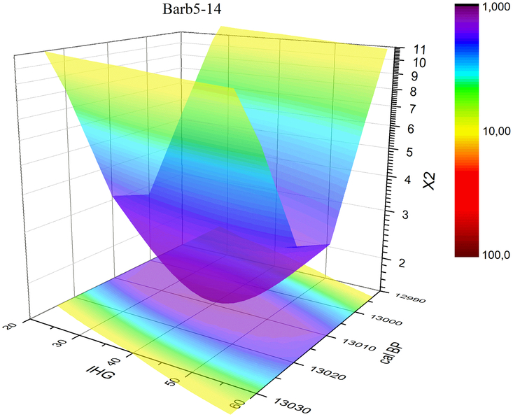
In Capano et al. (Reference Capano, Miramont, Guibal, Kromer, Tuna, Fagault and Bard2018), the dating of the Barbiers sequence was a preliminary determination based on a visual match with the kauri chronology (Hogg et al. Reference Hogg, Southon, Turney, Palmer, Bronk Ramsey, Fenwick, Boswijk, Friedrich, Helle, Hughen, Jones, Kromer, Noronha, Reynard, Staff and Wacker2016a, Reference Hogg, Southon, Turney, Palmer, Bronk Ramsey, Fenwick, Boswijk, Buüntgen, Friedrich, Helle, Hughen, Jones, Kromer, Noronha, Reinig, Reynard, Staff and Wacker2016b). For the present study, we used statistical analyses to compare and match the Barbiers and kauri series (i.e. R-cross-correlation coefficient, χ2 minimization and the Bayesian statistics tool of the OxCal program). The χ2 value varies with both the placement year and the 14C-IHG value, allowing χ2 minimization with both unknown variables (resulting in a surface in 3D plots such as in Figure 4).
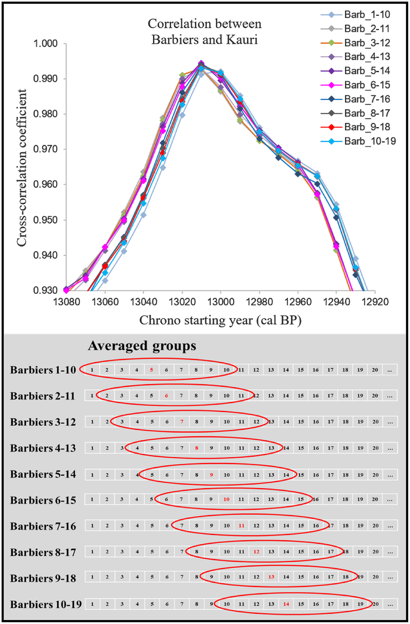
In order to compare our annual-resolution data with decadal-average data from kauri, we compared both records by averaging the Barbiers record to mimic the resolution of the kauri record. For each decade, we calculated the weighted average of the Barbiers 14C data included in the studied decade and the weighted error of the 14C data as the uncertainty for the decadal estimate. The starting year is arbitrary when calculating the Barbiers decadal average. We thus considered all possibilities leading to 10 averaged Barbiers curves, which were then compared with the kauri sequence (the first option starting from rings number #1 to 10 in the sequence, while other options differ by one ring numbers #2-11, #3-12 etc.; Figure 2).

Figure 2 Top: results of the cross-correlation coefficient for the 10 averaged groups of Barbiers series compared against the kauri record. Bottom: the averaging system used for obtaining the 10 groups.
RESULTS
Results of 14C Dating of the Barbiers Series
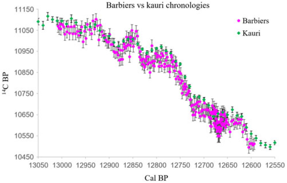
The 14C results for the Barb14 tree confirm its dendrochronological match with the Barb12 series, 14C-dated in Capano et al. (Reference Capano, Miramont, Guibal, Kromer, Tuna, Fagault and Bard2018; Figure 1). The dendrochronological position of the well-synchronized trees Barb13 and Barb14 is also confirmed with the new 14C results (Figure 1). The 14C dating confirms the dendro-match between Barb30 and BARB, attested by a high correlation coefficient, but short overlap (Table 1). Overall, this confirms the usefulness of considering 14C data at annual resolution for a more precise synchronization of series characterized by the irregular ring growth typical of the YD event (Figure 1).
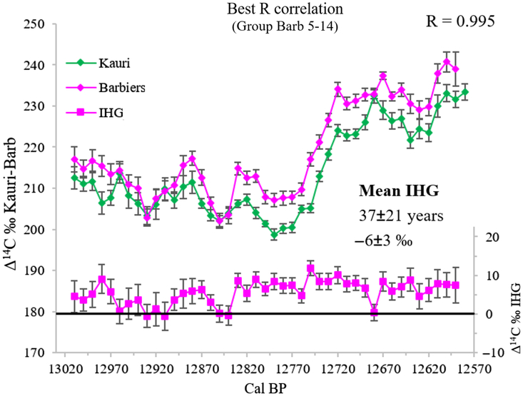
Optimization of the cross-correlation coefficient between the Barbiers decadal average curves and the kauri decadal curve shows slightly different optimum results, with the highest correlation observed when the Barbiers series starts at 13,008 cal BP with a decadal average starting with rings number #5 to 14 and so forth (Figures 2 and 3). In fact, all 10 options for averaging Barbiers exhibit high R values (>0.9) and we took this 10-yr range as a conservative error on the Barbiers chronology starting at 13,008 ± 5 and ending at 12,594 ± 5 cal BP (Figure 5).

Figure 3 Δ14C ‰ of Barbiers averaged groups compared against kauri record. The best dating position of Barbiers chronology obtained from the cross-correlation coefficient is given for each group. The best R value is obtained for the group 5-14. The IHG is shown for all groups compared with kauri (lower part of each graph).
The 10 decadal average series for Barbiers and the kauri chronology have been used to calculate the χ2 distance, which is minimum when the Barbiers series starts at 13,008 cal BP (option starting with the rings number #5-14 average; Figures 2 and 4). As for the optimization of the correlation coefficient, we take the 10-yr range of the different decadal averages as a conservative uncertainty for the placement of the Barbiers series: 13,008–12,594 ± 5 cal BP (Figure 5). As descibed below, the χ2 minimization also provides an optimal value for the IHG.

Figure 4 3D representation of the best dating option obtained by comparing Barbiers averaged series with kauri record by means of a χ2 test. The obtained combination of results suggests that the Barbiers chronology starts at 13,008 cal BP and that the mean IHG value is 40 yr.

Figure 5 Comparison between the Barbiers and the kauri chronology for the Younger Dryas period. The published kauri chronology (Hogg et al. Reference Hogg, Southon, Turney, Palmer, Bronk Ramsey, Fenwick, Boswijk, Friedrich, Helle, Hughen, Jones, Kromer, Noronha, Reynard, Staff and Wacker2016a, Reference Hogg, Southon, Turney, Palmer, Bronk Ramsey, Fenwick, Boswijk, Buüntgen, Friedrich, Helle, Hughen, Jones, Kromer, Noronha, Reinig, Reynard, Staff and Wacker2016b) is shifted by 10 yr towards older ages (Sookdeo et al. Reference Sookdeo, Wacker, Adolphi, Beer, Büntgen, Friedrich, Helle, Hogg, Kromer, Muscheler, Nievergelt, Palmer, Pauly, Reinig, Turney and Synal2019).
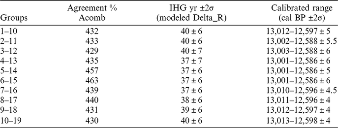
Finally, we compared the Barbiers and kauri chronologies by means of the Oxcal statistical program (Bronk Ramsey et al. Reference Bronk Ramsey, van der Plicht and Weninger2001) (Figure 6). The comparison was performed using the OxCal “Delta_R” uniform function (U(-120,120); Bronk Ramsey Reference Bronk Ramsey2009) in order to account for the IHG. The 10 average options for Barbiers were compared with the kauri chronology, leading to an optimal placement of 13,001–12,586 ± 6 Cal BP (2σ error; Table 2). As for the two previous techniques, we kept all 10 possible solutions as they show similar levels of agreement (Table 2). The youngest and oldest years of the 10 dating solutions lead to a range of 20 yr. This allows to date the Barbiers sequence to 13,006–12,591 ± 10 cal BP.
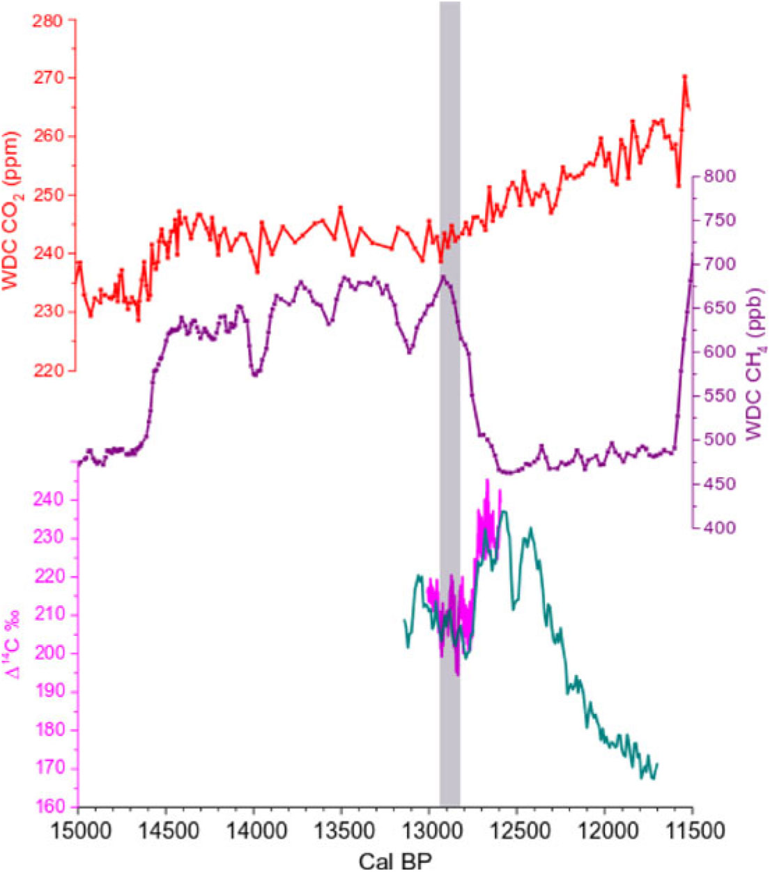
Figure 6 Comparison between Antarctica WDC CO2 data (red curve, top of graph) on the WD2014 age-scale (Marcott et al. Reference Marcott, Bauska, Buizert, Steig, Rosen, Cuffey, Fudge, Severinghaus, Ahn, Kalk, McConnell, Sowers, Taylor, White and Brook2014; Buizert et al. Reference Buizert, Cuffey, Severinghaus, Baggenstos, Fudge, Steig, Markle, Winstrup, Rhodes, Brook, Sowers, Clow, Cheng, Edwards, Sigl, McConnell and Taylor2015), Antarctica WDC CH4 data (purple curve, middle of graph) on the WD2014 age-scale (Marcott et al. Reference Marcott, Bauska, Buizert, Steig, Rosen, Cuffey, Fudge, Severinghaus, Ahn, Kalk, McConnell, Sowers, Taylor, White and Brook2014; Buizert et al. Reference Buizert, Cuffey, Severinghaus, Baggenstos, Fudge, Steig, Markle, Winstrup, Rhodes, Brook, Sowers, Clow, Cheng, Edwards, Sigl, McConnell and Taylor2015), and Δ14C‰ from New Zealand kauri trees and French Barbiers trees (green and pink curves, respectively, bottom of graph; from Hogg et al. 2016a and the present study). The gray band highlights the collapse of the IHG between 12,960–12,840 cal BP, which corresponds to the rise of pCO2 and the drastic drop of CH4 at the onset of the Younger Dryas cold period.
Table 2 Results of the comparison between the 10 averaged groups of Barbiers series and kauri record obtained by using OxCal program. IHG values in 14C yr are obtained by using a uniform Delta_R function (U(-120,120)). Calibrated ranges refer to the first and last years of the chronology for each group.
The OxCal Offset function also allows to compare the non-averaged series of Barbiers directly with the decadal record of Kauri. This leads to a chronology date of 13,003–12,588 ±25 cal BP (2σ error range). This dating option agrees with previous estimations, but has a somewhat larger uncertainty, which is linked to the different resolutions of the Barbiers and Kauri datasets.
Overall, the three statistical techniques (cross-correlograms, χ2 minimization and OxCal Delta_R) provide very similar results for the dating of Barbiers chronology. Taking the largest uncertainty, we can date our sequence to 13,008–12,594 ±10 cal BP. A higher precision for the dating of Barbiers chronology will become possible only when an annual-resolution 14C series of kauri chronology or any other absolutely dated 14C series for the YD period become available.
The existence of a brief Δ14C excursion at ca. 12,670 cal BP (12,680 cal BP with the new kauri placement by Sookdeo et al. Reference Sookdeo, Wacker, Adolphi, Beer, Büntgen, Friedrich, Helle, Hogg, Kromer, Muscheler, Nievergelt, Palmer, Pauly, Reinig, Turney and Synal2019) was suggested in our previous work (Capano et al. Reference Capano, Miramont, Guibal, Kromer, Tuna, Fagault and Bard2018). To evaluate the possibility of a solar event, we have improved the Barbiers 14C record specifically with the Barb17 tree: 14C was measured for every year from rings number #72 to 108 with at least two replicates for rings number #80 to 100 and 102, 105 (Table S1, Figure 1). The high resolution 14C record is characterized by rather noisy 14C values before and during the 14C peak, which makes it difficult to maintain the hypothesis of a sharp solar event.
Results on the Atmospheric 14C IHG
Lerman et al. (Reference Lerman, Mook, Vogel and Olsson1970) were the first to identify the presence of a small but systematic 14C difference between wood from trees that lived at the exact same time in the NH and SH (SH wood being 36 ± 8 yr older than NH wood). This 14C-IHG is maintained principally by air-sea CO2 exchange with the ocean surface that is typically much older than the atmosphere (from 400 to 1200 yr, Bard Reference Bard1988). Indeed, there is proportionally more ocean surface in the SH than in the NH, and the Southern Ocean is also characterized by generalized upwelling of old water and intense CO2 piston velocity due to extreme winds in the 40° to 60°S latitude belt (Levin et al. Reference Levin, Kromer, Wagenbach and Munnich1987; Braziunas et al. Reference Braziunas, Fung and Stuiver1995). The 14C-IHG is even more complex for trees grown after the Industrial Revolution due to anthropogenic fossil CO2 which has since been emitted mainly in the NH (Stuiver and Braziunas Reference Stuiver and Braziunas1998; McCormac et al. Reference McCormac, Hogg, Higham, Baillie, Palmer, Xiong, Pilcher, Brown and Hoper1998), thus disturbing and reversing the gradient.
Following Lerman et al. (Reference Lerman, Mook, Vogel and Olsson1970), several other authors have further quantified the IHG. Hogg et al. (Reference Hogg, McCormac, Higham, Reimer, Baillie and Palmer2002) measured the 14C-IHG over the last millennium, deriving an average value of 40 ± 13 yr and suggesting a 130-yr periodicity for 14C-IHG variations. Taking into account the variability of the 14C-IHG, McCormac et al. (Reference McCormac, Hogg, Blackwell, Buck, Higham and Reimer2004) proposed using a modeled 14C-IHG of 56–58 yr for the SH calibration curve (SHCal04), with a variability of ±8 yr at 1000 cal BP and ±25 yr at 11,000 cal BP.
Hogg et al. (Reference Hogg, Southon, Turney, Palmer, Bronk Ramsey, Fenwick, Boswijk, Friedrich, Helle, Hughen, Jones, Kromer, Noronha, Reynard, Staff and Wacker2016a) calculated the 14C-IHG for most of the YD event. They found variable values (averaged to 38 ± 6 yr), which are generally in agreement with the data for the last two millennia (44 ± 17 yr; Hogg et al. Reference Hogg, Palmer, Boswijk and Chris2011). The same authors also described a collapse of the 14C-IHG during the period between 13,100 and 12,660 cal BP (Hogg et al. Reference Hogg, Southon, Turney, Palmer, Bronk Ramsey, Fenwick, Boswijk, Friedrich, Helle, Hughen, Jones, Kromer, Noronha, Reynard, Staff and Wacker2016a). However, annual-resolution 14C data from French trees spanning the early part of the YD around 12,660 cal BP indicate that the 14C-IHG was similar to the modeled value calculated by McCormac et al. (Reference McCormac, Hogg, Blackwell, Buck, Higham and Reimer2004), with no evidence of a collapse (Capano et al. Reference Capano, Miramont, Guibal, Kromer, Tuna, Fagault and Bard2018).
For this study we can evaluate the 14C-IHG with the Barbiers record, extended to 415-yr with improved resolution with respect to our previous publication (Capano et al. Reference Capano, Miramont, Guibal, Kromer, Tuna, Fagault and Bard2018). To calculate the 14C-IHG, the Barbiers data from the NH were compared to the kauri data from the SH. As explained in the previous section dealing with chronological placement, Barbiers is averaged 10 times at decadal resolution and the 14C-IHG calculation was performed at this same resolution, leading to 42–43 estimations, depending on the averaged curve. Considering the optimum correlation coefficient R for each of the 10 options, the 14C-IHG was then calculated by subtracting the Barbiers 14C age and Δ14C ‰ from the corresponding kauri decadal 14C-age and Δ14C values (Δt = (14C age)kauri – (14C age)Barb, ΔΔ14C = Δ14Ckauri – Δ14CBarb). Note that the ratio between the 14C-IHG in age and in ‰ is not strictly constant. This is due to the fact that both Δ14C values are elevated and vary through time (N.B. if the Δ14C values were close to 0, the Taylor series approximation of Ln(1+x) = x at first order would lead to Δt = –8·ΔΔ14C).
The 14C-IHG shows mean values ranging between 31 yr with a SD of 23 yr and 43 yr with a SD of 23 yr, depending on the chronological placement (–5 to –7‰). Minimizing the χ2 distance provides a direct estimation of the 14C-IHG (Figure 4). Depending on the chronological placement, the optimum IHG value varies from 34 to 46 yr (–5 to –7‰). Matching the Barbiers and kauri decadal records with the Oxcal program, also provides a direct 14C-IHG estimation, which ranges between 37 and 40 yr (–6‰; Table 2). Overall, the three statistical techniques provide similar 14C-IHG values.
Considering only the best chronological placement, 13,008–12,594 ±10 cal BP, the mean 14C-IHG value is 37 yr with a SD of 21 yr (n = 43), –6‰ with a SD of 3‰ (Figure 3). The 14C-IHG time variations in Figure 3 indicate two periods with minimal values close to 0 from 12,960 to 12,900 cal BP and from 12,860 to 12,840 cal BP, where the 14C-IHG oscillates between –4 and 24 yr (between 1 and –4‰):
During the first period (12,960–12,900 cal BP) the mean 14C-IHG is 10 yr with a SD of 12 yr (n = 7), –2‰ with a SD of 2‰.
During the second period (12,860–12,840 cal BP), the mean 14C-IHG is 6 yr with a SD of 12 yr (n = 3), –1‰ with a SD of 2‰.
The period in-between (12,890–12,870 cal BP) shows a value of 39 yr with a SD of 4 yr (n = 3), –6‰ with a SD of 1‰, in agreement with the overall mean 14C-IHG of 37 yr.
These intervals with minimum 14C-IHG correspond in time to the beginning of the YD event at 12,846 ± 138 cal BP (Rasmussen et al. Reference Rasmussen, Andersen, Svensson, Steffensen, Vinther, Clausen, Siggaard-Andersen, Johnsen, Larsen, Dahl-Jensen, Bigler, Röthlisberger, Fischer, Goto-Azuma, Hansson and Ruth2006).
By excluding the two short periods with minimal 14C-IHG, it is possible to recalculate a mean 14C-IHG of 45 yr with a SD of 14 yr (n = 33), –7‰ with a SD of 2‰. These values are indistinguishable from the 14C-IHG observed over the last two millennia (44 yr with a SD of 17 yr; Hogg et al. Reference Hogg, Palmer, Boswijk and Chris2011).
The plot of 14C age versus calendar ages (Figures 1, 5) exhibits three “age plateaux” during the periods 13,010–12,970 cal BP, at the beginning of the Barbiers chronology, 12,820–12,770 cal BP, immediately before the drastic Δ14C rise, and 12,720–12,690 cal BP, immediately after the Δ14C rise. The 14C-IHG determination is expected to be particularly robust during these periods. Indeed, a slight inaccuracy in the chronological placement of the Barbiers sequence with respect to the kauri record would not affect the 14C difference over an “age plateau.” The IHG during the three “age plateaux” is the following:
Over the 13,010–12,970 cal BP “plateau” the 14C-IHG average is 37 yr with a SD of 14 yr (–6 with a SD of 2‰; n = 5).
For the 12,820–12,770 cal BP “plateau” the 14C-IHG average is 49 yr with a SD of 9 yr (–7‰ with a SD of 1‰; n = 6).
During the 12,720–12,690 cal BP plateau the 14C-IHG average is 53 yr with a SD of 9 yr (–8‰ with a SD of 1‰; n = 4).
During each of the three “plateaux,” the individual decadal 14C-IHG values are fully compatible with each other. It is thus reasonable to assume that the 14C-IHG was stable during these periods. Under this hypothesis, we can calculate one sigma errors of the mean (SE = SD/√n) for the 14C-IHG determinations: 37 ± 6 yr, 49 ± 4 and 53 ± 5 yr, respectively for the three 14C “age plateaux” in chronological order. The data suggest that the first 14C-IHG value is thus statistically lower than the two other values. This may indicate that the IHG increased during the transition between the Allerød and the YD periods at around 12,846 cal BP, but, more 14C data will obviously be needed to verify this suggestion. An additional problem is that the uncertainty on the climatic transition is large (±138 yr in the Greenland ice GICC05 chronology). Identification of this transition directly in the trees would certainly help to resolve the issue.
The period between 12,760 and 12,730 cal BP is characterized by a drastic Δ14C rise of 25‰. However, the 14C-IHG remains high, with a mean of 55 yr, and relatively stable, with a SD of 19 yr based on 4 values (–8‰ and a SD of 3‰). This translates to an 14C-IHG estimate of 55 yr and SE of 10 yr, which agrees with the overall mean and SE of 45 ± 2 yr (excluding the two brief periods of minimal IHG).
The 14C-IHG in subfossil trees reflects the asymmetry between the 14C signatures of CO2 fluxes to the atmosphere in the SH and NH. Variations of the 14C-IHG are thus to be expected when the N-S balance of CO2 fluxes is perturbed in both ocean and land sources. For example, Rodgers et al. (Reference Rodgers, Mikaloff-Fletcher, Bianchi, Beaulieu, Galbraith, Gnanadesikan, Hogg, Iudicone, Lintner, Naegler, Reimer, Sarmiento and Slater2011) used an ocean-atmosphere model to study the 14C-IHG variations over the last millennium and attributed an abrupt 14C-IHG decrease by 16 yr (2‰ in Δ14C) to a weakening of the Westerlies in the Southern Ocean.
The new 14C record of Barbiers trees suggests a 14C-IHG increase between the end of the Allerød (IHG = 37 ± 6 yr) and the early YD (IHG = 48 ± 3 yr). This is compatible with ocean circulation changes, namely: a decrease in deep-water convection in the North-Atlantic and an associated increase in wind-driven upwelling in the Southern Ocean.
The new 14C-IHG record also shows a 120-yr period (12,960–12,840 cal BP) characterized by two brief phases of minimal values followed by the YD increase: the first of these phases lasted 6 decades, while the second was shorter, spanning 2 decades only. It is reasonable to hypothesize that these century-long anomalies in 14C-IHG are in fact synchronous with the start of the YD event.
It is also important to note that the 14C-IHG minima are also synchronous with Δ14C minima in both the NH and SH. This suggests that this century-long period was characterized by a strong release of relatively old CO2, preferably into the NH atmosphere. The timing of the Δ14C decrease would thus correspond to the start of the rise in atmospheric CO2 that occurred at the beginning of the YD (Figure 6).
Further analyses are needed to confirm our observations, together with carbon cycle modeling to simulate the triple isotope signatures and the 14C-IHG. Between 13,000 and 12,800 cal BP, atmospheric Δ14C is rather stable, but exhibits century-long cycles with minima corresponding to the two 14C-IHG anomalies. It will be important to evaluate the possible variations of the 14C production during this period by comparing the observed Δ14C variations with those in the 10Be record from ice cores (e.g. Bard et al. Reference Bard, Raisbeck, Yiou and Jouzel1997; Adolphi et al. Reference Adolphi, Bronk Ramsey, Erhardt, Lawrence Edwards, Cheng, Turney, Cooper, Svensson, Rasmussen, Fischer and Muscheler2018). Nevertheless, cosmogenic production changes through solar modulation should affect both hemispheres in a rather symmetric way. Hence, CO2 fluxes in the NH from old carbon oxidation can be seen as a possible mechanism to explain the observed variations.
CONCLUSIONS
We have analyzed a 416-yr-long tree-ring chronology from subfossil trees (Pinus sylvestris L.) which grew in the southern French Alps during the Younger Dryas cold period. 14C measurements at annual resolution of this Barbiers chronology were performed at least every third year of the sequence, establishing a high-resolution 14C sequence in a period characterized by tree growth recession.
We date the new Barbiers record to 13,008–12,594 ±10 cal BP by matching the 14C patterns with those of the kauri chronology. Consequently, the Barbiers record should include the transition between the Allerød and YD events at 12,846 cal BP, although the exact position of the boundary is still uncertain due to the error of the ice core chronology (138 yr).
Our new data allow to calculate the 14C-IHG between the Northern Hemisphere (Barbiers pines from France) and the Southern Hemisphere (kauri trees from New Zealand). The mean 14C-IHG is 37 yr with a SD of 21 yr based on 43 decadal estimations.
Over the 415 yr, the 14C-IHG exhibit minimal values of between 12,960–12,840 cal BP. Excluding these minima from the average, leads to a mean 14C-IHG of 45 yr with a SD of 14 yr based on 33 decadal values, in agreement with observations for the last two millennia.
The Barbiers record suggests a 14C-IHG increase between the end of the Allerød period (IHG = 37 ± 6 yr) and the early part of the YD (IHG = 48 ± 3 yr). This change is compatible with a previously reported drop of deep-water convection in the North-Atlantic and an associated increase in wind-driven upwelling in the Southern Ocean.
Between 12,960 and 12,840 cal BP the 14C-IHG minima are accompanied by Δ14C minima in both the NH and SH. These data have been compared with the records of CO2 and CH4 mixing ratios measured in air bubbles occluded in Antarctic ice. The concomitant 14C-IHG and Δ14C minima seem to correspond to the start of the rise in atmospheric CO2 and the decrease in CH4 at the beginning of the YD.
Further work is needed using carbon cycle modeling to simulate the various carbon isotope signatures, so as to take into account possible variations of 14C production during this period by considering variations in the 10Be ice core record.
ACKNOWLEDGMENTS
AixMICADAS and its operation are funded by the Collège de France, the EQUIPEX ASTER-CEREGE and the ANR project CARBOTRYDH (PI E.B.).
SUPPLEMENTARY MATERIAL
To view supplementary material for this article, please visit https://doi.org/10.1017/RDC.2019.116