INTRODUCTION
In the deserts and drylands of Baja California, cardon (Pachycereus pringlei) is the most widely distributed columnar cactus. It can reach extraordinary heights (16–20 m) in some parts of the peninsula, and is considered to be among the longest-lived columnar cacti (Turner et al. Reference Turner, Bowers and Burgess1995; Bullock et al. Reference Bullock, Martijena, Webb and Turner2005; Medel-Narváez et al. Reference Medel-Narváez, de-la-Luz, Freaner-Martinez and Molina-Freaner2006). The annual elongation rate of the main shoots of cardon has been measured in controlled experiments with added watering for ~8 yr, with estimates ranging between 14 and 23 cm/yr (Nerd et al. Reference Nerd, Raveh and Mizrahi1993; Suzán-Azpiri and Sosa Reference Suzán-Azpiri and Sosa2006). Other authors, however, have suggested that under natural conditions the shoot elongation rate is lower (Bashan et al. Reference Bashan, Toledo and Holguin1995; Bacilio et al. Reference Bacilio, Vazquez and Bashan2011).
English et al. (Reference English, Dettman, Sandquist and Williams2007, Reference English, Dettman, Sandquist and Willams2010) used radiocarbon dating and stable isotope analysis of saguaro cactus (Carnegiea gigantea) spines to examine how the photosynthetic physiology of this plant, associated with variation in the δ13C values of spines, changed with time. The chronology was based on the 14C age of a subset of the sampled spines. Among other results, they found a high correlation (r=0.99) between the 14C age of spines and the measured height of the plants over the preceding 4 decades. 14C dating of plant tissues to estimate the age of plants has been used with other long-lived species that lack visible growth rings. For example, López-Medellín et al. (Reference López-Medellín, Ezcurra, González-Abraham, Hak, Santiago and Sickman2011) were able to estimate the age of mangrove trees by 14C dating the cellulose in the pith at the base of the main stem.
In cardon, as in other columnar cacti, spines develop sequentially from the apex, which, as it grows, initiates lateral axillary buds subtended by diminutive microscopic leaves. Cactus spines are the highly modified bracts of the axillary buds, called areoles in cacti. Despite their foliar origin, cactus spines differ considerably from the leaves and bracts of most dicots. They consist of a core of dense woody fibers surrounded by sclereid-like epidermal cells. Cells in the spines die as the spine forms, and living cells only occur at the base of the spine. Thus, spines are highly modified structures, composed of dead woody fibers and sclereids with highly lignified secondary walls, and form shortly after the apical meristem of the shoot initiates a new lateral bud. Spines, however, lack vessel cells and, in contrast with true wood, once formed they do not exchange any organic materials with the rest of the plant, retaining their original structure until the whole areole is shed off or until the whole plant dies (Mauseth Reference Mauseth2006). This makes spines ideal subjects for 14C dating analysis, as they develop close to the tip of the central shoot meristem in a matter of a few weeks (in the saguaro cactus, for example, spines reach full development in 30–60 days; English et al. Reference English, Dettman, Sandquist and Willams2010) and, once formed, they do not receive any new carbon input from the plant’s living tissues (English et al. Reference English, Dettman, Sandquist and Williams2007).
This article reports the 14C ages of 25 individuals of giant cardon in six sites distributed throughout the peninsula of Baja California. Our objectives were to (a) establish with precision the age of each individual using spine 14C dating, (b) calculate the mean annual growth rate of the lead shoot in each individual, and (c) correlate the measured growth rates with both plant and environmental predictors, such as plant size, precipitation, population density, water availability, or latitude. Our main hypothesis was that the dead tissue of spines can be used to date the age of giant columnar cacti using 14C methods. We also wanted to test whether allometric variables, such as plant size, or site-specific environmental variables, such as water availability, had an influence on the plants’ overall growth in height.
METHODS
Sampling Sites
We selected six sites along the Gulf coast slope of Baja California, from latitude 22.8° to 31.3°N, and explored the whole range of precipitation in which the species grows, from 55.3 to 517.9 mm of mean annual precipitation according to historical (1951–2010) records from Mexican weather stations (CONAGUA 2010; see Figure 1). All sites are flat and with relatively low slopes (<4%), and lie in the eastern divide of the peninsula, facing towards the Gulf of California in order to minimize the potential effect of additional moisture derived from Pacific Ocean fog.
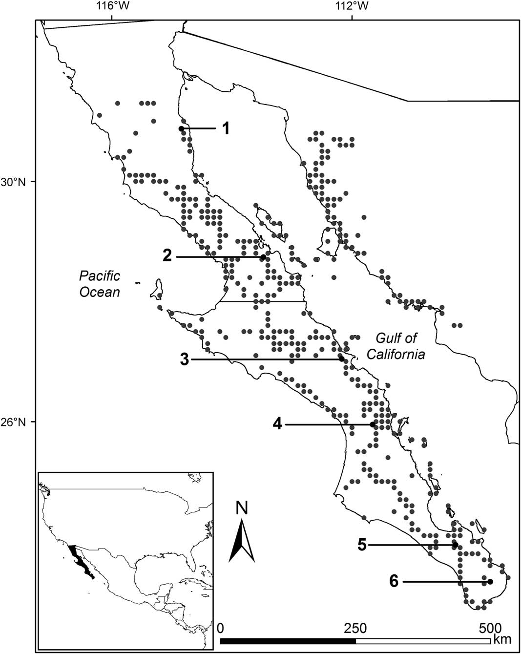
Figure 1 Sampling sites and geographic range of cardon. Gray points show observation/collection sites taken from Turner et al. (Reference Turner, Bowers and Burgess1995). The six black points show the study sites: (1) Percebú (30.88°N, –114.76°W), (2) San Borja (28.75°N, –113.76°W), (3) San José de Magdalena (27.09°N, –112.19°W), (4) San Javier (25.90°N, –111.54°W), (5) San Pedro (23.92°N, –110.28°W), and (6) Mangle (23.34°N, –109.64°W). Mean annual precipitation at the six sites for the period 1951–2010 was (1) 55.3 mm, (2): 114.1 mm, (3): 180 mm, (4): 297.1 mm, (5): 335.1 mm, and (6): 517.9 mm; site elevation is (1): 35 m, (2): 419 m, (3): 144 m, (4): 459 m, (5): 171 m, and (6): 289 m; and the number of individuals per hectare was (1): 39, (2): 187, (3): 50, (4): 157, (5): 57, and (6): 255.
In each site, we established a 1-ha plot (100 m×100 m) less than 6 km away from the nearest weather station and harboring populations of cardon cactus (Pachycereus pringlei), whose general physiognomy did not differ appreciably in density or mean height from those in the larger landscape. In each plot, we counted all individual plants present and registered their height using a forester’s hypsometer (Nikon Forestry 550, Nikon Vision Co., Tokyo, Japan).
Sampling Methods
Within the plot, we chose four individuals, each belonging as nearly as possible to a different height category (2, 4, 6, and 8 m). In site 1 (Percebú), where unusually tall plants were found, we added a fifth individual of 13.5 m in height. In each individual, we identified the lowermost intact areole and collected one of the central spines of the areolar cluster for 14C dating. Care was taken to avoid damaged areoles with younger, regrown spines, easily identifiable by their smaller size, sparser number, irregular whorl arrangement, and lighter color. We measured the height of the sampled areole to the ground and the total height of the plant from ground level to the tip of the highest stem.
Radiocarbon Dating and Calibration
Each spine was wrapped in aluminum foil and stored in a dry environment before sending to the W. M. Keck Carbon Cycle Accelerator Mass Spectrometry (KCCAMS) lab in the Department of Earth Systems Science at the University of California, Irvine, for 14C dating (Southon and Santos Reference Southon and Santos2004, the protocol can be found at www.ess.uci.edu/researchgrp/ams/protocols).
Because many spines are more recent than 1951, the year in which open-air nuclear tests started to have significant effects on the levels of 14C in the atmosphere, we followed Reimer et al.’s (Reference Reimer, Brown and Reimer2004) fraction modern (F14C) approach for calibration of post-bomb Δ14C data, using the CALIBomb online calibrator (http://calib.qub.ac.uk/CALIBomb/), with the IntCal13 atmospheric data set (Reimer et al. Reference Reimer, Bard, Bayliss, Beck, Blackwell, Bronk Ramsey, Brown, Buck, Edwards, Friedrich, Grootes, Guilderson, Haflidason, Hajdas, Hatté, Heaton, Hogg, Hughen, Kaiser, Kromer, Manning, Reimer, Richards, Scott, Southon, Turney and van der Plicht2013) and the NHZ2 bomb curve extension (Hua et al. Reference Hua, Barbetti and Rakowski2013).
Height-Specific Growth Rates
From each plant, we obtained three age-related data: (a) the height at the tip of the tallest shoot of the plant (h p ), (b) the height of the lowest spine (h s ), and (c) the calibrated 14C date for the time when the lowest spine was formed (Δt), which corresponds to the difference between the age of the plant at the time at which the spine was formed (t s ) and the current age of the plant (t p ). From these values, we estimated the mean annual growth rate (ρ) of the plant during the time interval Δt as ρ=(h p – h s )/(t p – t s ), or Δh/Δt. These height-specific growth rates can be regressed against the height of the plant (h p ), and a simple linear function can be fitted relating the growth rates as a function of plant height. If the growth rate ρ is associated to the plant’s size, then the expected growth rate will follow a linear model (ρ=a + bh), in its simplest case, or a higher-order polynomial if the relationship between growth rate and height is curvilinear.
Once the mean annual growth rates of the individual plants were calculated, we performed an analysis of covariance (ANCOVA) with growth rates as the dependent variable, plant height (h p ) as the covariate, and a series of independent variables as additional predictors, including environmental factors and variables (site, mean annual rainfall, summer rainfall, annual per capita water availability, distance to the coast of the Pacific Ocean, altitude, and latitude), as well as two population-related variables (density and maximum height of all plants in the site). The ANCOVA and all other statistical tests were done using the R program (R Core Team 2015).
Estimating Plant Age
After finding that, indeed, the growth rate was linearly associated with the plant’s height, the age of the plant at the time the lowest spine was produced was calculated by simple extrapolation. Bearing in mind our simple growth rate versus height model ρ=a + bh, and recalling that, by definition, ρ=Δh/Δt, we used the regression parameters to calculate the age of the lowest spine (t s ). Between plant germination and the formation of the lowest spine, the changes in height and age can be calculated as Δh s =(h s – 0) and Δt s =(t s – 0). Then, it follows that
 $${{{\vartriangle} Δ h_{s} } \over {{\vartriangle} Δ t_{s} }}={{h_{s} } \over {t_{s} }}= a{\plus}bh_{s} $$
and, solving for t s , the age of the plant at height h s can be estimated as
 $$t_{s} ={{h_{s} } \over {a{\plus}b.h_{s} }}$$
Finally, we added the estimated age of the plant when the lowest areole was produced to the 14C age of the lower spine to obtain an estimate of t p , the plant’s age, calculated as t p =t s + Δt.
Plant Height Versus Age Model
The ANCOVA model demonstrated that the mean growth rate in the interval between the age of the lowest spine and today was linearly related to the plant’s height. These mean rates were ascribed to the midpoint age of the plant [the point {t
m
, h
m
} in Figure 2], defined as the age in which the annual growth rate (dh/dt) equaled the long-term mean rate ρ=Δh/Δt (the exact derivation of the coordinates for the midpoint are presented in the Appendix). Because the midpoint height is a fraction of the total height, there was also a strong correlation between the mean growth rate for each plant and the height at the point in which that rate was reached. This relationship can be written in the form of a differential equation, such that
 ${{dh} \over {dt}}= a {\plus} bh$
.
${{dh} \over {dt}}= a {\plus} bh$
.
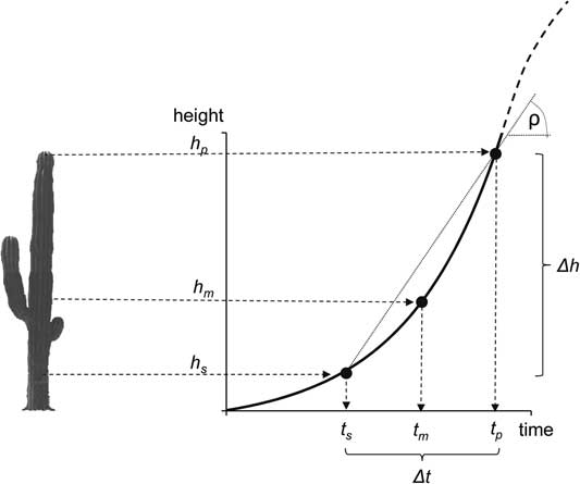
Figure 2 Conceptual diagram of the parameters measured in each plant: plant height (h p ), height of the lowest spine (h s ), and 14C age of the lowest spine (Δt). With these values, we estimated the plant’s mean annual growth rate [ρ=(h p –h s )/Δt], the height at which the plant achieved that growth rate (h m ), the age of the plant at the height where the lowest spine was formed (t s ), and the age of the plant (t p =t s + Δt).
This equation can be rewritten as
 $dh/(a{\plus}bh)=dt$
, and integrating both sides, we get
$dh/(a{\plus}bh)=dt$
, and integrating both sides, we get
 ${\rm ln}(a {\plus} bh) = {\rm ln}(a) {\plus} bt$
. Solving for h, we get the final model
${\rm ln}(a {\plus} bh) = {\rm ln}(a) {\plus} bt$
. Solving for h, we get the final model
 $$h = {a \over b}(e^{{b.t}} -1)$$
which predicts the expected height of the plant as a function of age (t). Because the plant’s age-height relationship is based on the linear regression coefficients a and b, the standard error of the coefficients can be used to get confidence intervals. Algebraic details on the derivation of the models and on estimation of the parameters are given in the Appendix.
RESULTS
Radiocarbon Results
The spines of only two individuals, one in site 1 (Percebú 742) and a second one in site 2 (San Borja 177), gave ages before 1950 (pre-bomb). All other spines were formed after 1950 (Table 1).
Table 1 Site and individual code, plant height (h p ), height of the collected spine (h s ), Keck Lab dating code (UCI-AMS), ratio of stable isotopes 13C:12C (δ13C), fraction modern 14C value (F14C), estimated age range of the spine (2σ AD, the probability value is given in parentheses), estimated age of the lowest spine, mean annual growth rate (ρ), and estimated age of the individual.

Height-Specific Growth Rates
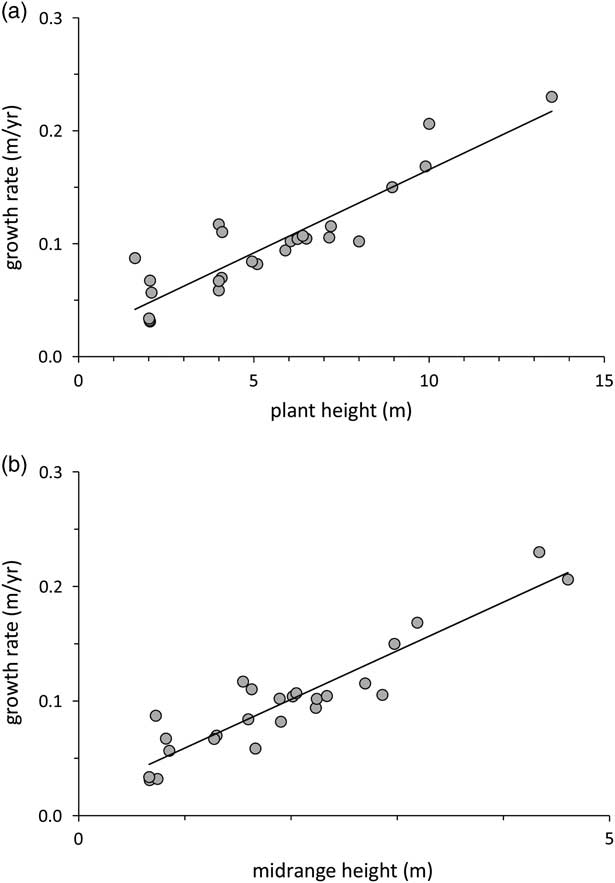
Mean annual growth rates varied considerably, from 3 to 23 cm/yr in different plants. There was a very strong linear relationship between mean annual growth rate and the total height h p of the plant (r 2=0.82, P<0.0001), showing that, as individual plants grow, the annual rate of elongation of the leading shoot tends to increase at least until the plants reaches ~4 m (the highest value for any midpoint height h m in our data set; see Figure 3a). As a result, there was also a strong and significant correlation (r 2=0.85, P<0.0001) between the mean annual growth rate of the plant and the midpoint height h m at which that growth rate is estimated to have occurred (Figure 3b). An analysis of covariance failed to find any other significant relationship between mean annual growth rate and environmental characteristics of the site (total precipitation, summer precipitation, latitude, altitude, or distance to the Pacific coast) or characteristics of the population (density and maximum plant height).

Figure 3 (a) Correlation between the plant mean annual growth rate (ρ) and the total height of the plant (h p ). Larger plants show higher mean growth rates (y=0.0182 + 0.0147 x; r 2=0.82, F 2,23=105.9, P<0.00001). (b) Correlation between the plant’s mean annual growth rate (ρ) and the height of the plant at the point where the instantaneous growth rate equals the lifelong mean growth rate (h m ). The annual growth rate increases linearly with the midpoint height (y=0.0166 + 0.0424 x; r 2=0.85, F 2,23=133.7, P<0.00001).
Estimation of Plant Ages
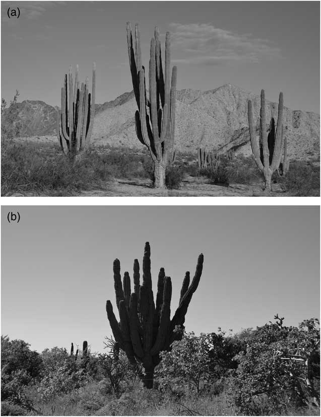
The estimated age of our sampled plants varied between 19.5 and 84.3 yr. The youngest plant was found in site 1 (Percebú) with 1.6 m in height and 19.5 yr of estimated age, and the oldest individual was found in site 5 (San Pedro) with 84.3 yr of age and a height of 7.1 m (Figure 4).

Figure 4 (a) The population in site 1 (Percebú) had the tallest individuals and the lowest density of any site. With a mean annual precipitation of ~50 mm, this was our driest site in the peninsula. It harbors a sparse creosote bush scrub and cardon cacti dominate over the landscape. (b) In site 5 (San Pedro), we registered the oldest individual (observable in the center of the image). The high precipitation in this site (>500 mm) allows the presence of a lush tropical dry scrub.
Age-Height Relationship
Our model, obtained from integrating the growth rate vs. age function, predicted an exponentially growing plant size until the cardon plants reach ~80 yr old (presumably, after that point height increase levels off, giving way to lateral branching, but our data set did not include plants old enough to model that part of the growth process in detail). Because plants differ in their mean long-term growth rates, the integrated error functions yielded a funnel-shaped distribution of the variance, showing that, despite the relatively narrow and highly significant linear relationship between annual growth rates and plant heights, relatively small variations in growth rates will accumulate as plants grow in such a way that plants of 60 yr of age may range in height from 2 to 14 m. The relationship between age and height in our sample data points also showed a very high dispersion of the data points, increasing as the plants grow in size and age (Figure 5). Although the model and the data points in Figure 5 coincide well, it is still unclear in our data set how much of the variation in plant height, given a certain age, is due to within site random variation or to fixed effects between sites.
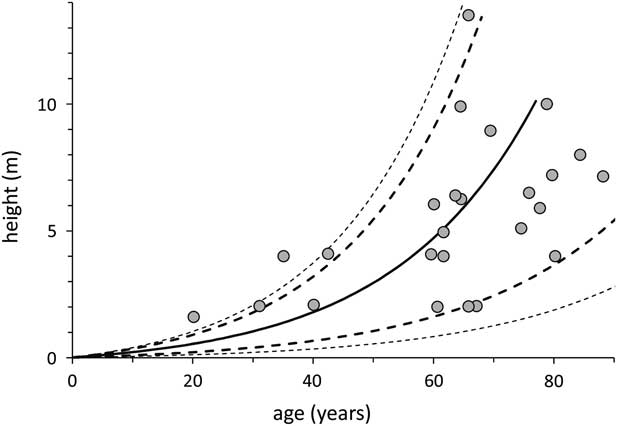
Figure 5 The height-age model obtained from integrating the growth rate equation shows the expected exponential growth of the stems from 0 to 6 m, but, more importantly, an expanding prediction error as the plants age. The data points correspond to the 25 sampled plants plotted according to their measured height and their 14C-estimated age. The continuous line is the model’s predicted height-to-age relationship, the bold broken lines correspond to the 5% confidence interval, and the outer, thinner lines to the 1% interval.
DISCUSSION
Age estimation has been repeatedly reported as a key factor in the study, management, and conservation of giant columnar cacti (Steenbergh and Lowe Reference Steenbergh and Lowe1977; Drezner Reference Drezner2003; Danzer and Drezner Reference Danzer and Drezner2010). Our results confirm the theoretical results of Bullock et al. (Reference Bullock, Turner, Hastings, Escoto-Rodríguez, Ramírez, López and Rodríguez-Navarro2004) who, using plant-growth models, showed that age estimates for giant cacti based on size and growth rates are subject to large errors when the interannual rates within a single individual are autocorrelated (i.e. when some individuals are consistently fast growers while others are consistently slow growers). Bullock et al. (Reference Bullock, Turner, Hastings, Escoto-Rodríguez, Ramírez, López and Rodríguez-Navarro2004) discuss that this inherent source of error in age estimates raises major problems for the ecological analysis and management of these plants, and underscore the need for more precise dating methods. 14C dating may provide a robust alternative method to estimate age and growth rates in columnar cacti.
Some studies on the demography of cardon have hypothesized that this species is possibly much longer lived than the large saguaro cactus (Carnegiea gigantea), for which ages derived from growth rates suggest a longevity of less than 200 yr (Bullock et al. Reference Bullock, Martijena, Webb and Turner2005; Pierson et al. Reference Pierson, Turner and Betancourt2013; Drezner Reference Drezner2014). Our results show that large (10–13 m) cardon plants can be less than a century in age, indicating that the growth rates of saguaro and cardon may be quite similar. However, because our sampling was not directed towards the oldest individuals in the sampled populations, our data do not allow us to make at this point an estimation of species longevity.
Growth rates in Pachycereus pringlei are strongly associated with plant height by a simple linear relationship (at least in the size categories we studied). As a consequence, plant height is related to plant age by an exponential relationship, at least in the younger plants as, presumably, older plants may eventually level off in their growth rates as their photosynthetic surplus becomes limited by decreasing surface-to-volume relationships and the plants start branching laterally. However, the error variance of the height-to-age prediction increases along the life history of the plants and, as plants grow taller, their age estimation becomes more and more uncertain, especially if elongation of the highest shoots tends to level off at a certain height. This fact may add another element in favor of 14C dating of plant age, as the only height-age estimation necessary with this method is below the level of the lowest areole, normally less than 1 m high, and within a range in which height-age predictions are still relatively accurate.
It is noteworthy that, apart from the strong association between annual growth rates and plant height, no other factor was identified in the ANCOVA as having a significant influence on growth rates. In particular, it was surprising to find that mean annual precipitation or per capita water availability were not predictors of plant growth rates, and that intrasite variation in individual growth rates was higher than between-site differences. This point warrants further and more detailed exploration, as the within-site sample size for this first study was low. Nonetheless, it is interesting to note that other studies (Turner et al. Reference Turner, Webb, Bowers and Hastings2003; Bullock et al. 2006) using repeat photography showed populations of tall Pachycereurs pringlei (5 m or more) in different parts of the Sonoran Desert arising in periods of less than 90 yr, a fact that implies mean annual growth rates of 0.05–0.10 m/yr, very similar to the ones reported in our study.
14C dating of cactus spines opens many possibilities for new research in cactus ecology, including (a) sampling single plants along their stem to understand their growth history in greater detail; (b) comparing in detail individual plants within a site, to understand intrapopulation variation; (c) study long-term plant growth in relation to atmospheric and oceanographic anomalies such as El Niño oscillations or long-term droughts; and (d) bring precise age-dating methods into studies of cactus morphology, branching patterns, and surface-volume relationships.
ACKNOWLEDGMENTS
We thank UC MEXUS, CONACYT, and CIBNOR for financial support, Christian Silva and Jonathan Escobar for field assistance, and the landowners for providing access to the research sites. We want to acknowledge the generous support and assistance of John Southon and the staff at the W. M. Keck Carbon Cycle Accelerator Mass Spectrometry Laboratory at UC Irvine. Additional logistical support was provided by Mayte Fernández and Oscar Delgado. Comments from two anonymous reviewers helped us to improve our manuscript.
Appendix. Estimation of the Parameters of the Height vs. Age Model
Growth rates. Growth rates were estimated from the three age-related parameters measured in each plant: (a) total height (h p ), (b) height of the lowest spine (h s ), and (c) radiocarbon age of the lowest spine (Δt). With these values, we estimated the mean growth rate (ρ) as ρ=(h p - h s )/Δt, or Δh/Δt.
Midpoints. The point {t
m
, h
m
} where the mean growth rate (ρ) equals the instantaneous rate (dh/dt) can be found analytically. Let us recall first that Δh=h
p
– h
s
, and that the model-predicted values for h
p
and h
s
are
 $h_{p} ={a \over b}(e^{{b.t_{p} }} -1)$
and
$h_{p} ={a \over b}(e^{{b.t_{p} }} -1)$
and
 $h_{s} ={a \over b}(e^{{b.t_{s} }} -1)$
. However, because t
p
=t
s
+ Δt, it follows that
$h_{s} ={a \over b}(e^{{b.t_{s} }} -1)$
. However, because t
p
=t
s
+ Δt, it follows that
 $$\Delta h= {a \over b}e^{{b.t_{s} }} (e^{{b.\Delta t}} {\minus}1)$$
. On the other hand, derivating Equation 3 with respect to time we find that the instantaneous growth rate at point t
m
is
$$\Delta h= {a \over b}e^{{b.t_{s} }} (e^{{b.\Delta t}} {\minus}1)$$
. On the other hand, derivating Equation 3 with respect to time we find that the instantaneous growth rate at point t
m
is
 $dh/dt=a.e^{{b.t_{m} }} $
. But point t
m
lies between t
s
and t
p
, so we can define a difference value δt such that t
m
=t
s
+ δt. Now the derivative equation becomes
$dh/dt=a.e^{{b.t_{m} }} $
. But point t
m
lies between t
s
and t
p
, so we can define a difference value δt such that t
m
=t
s
+ δt. Now the derivative equation becomes
 $dh/dt=a.e^{{b.t_{s} }} .e^{{b.\delta t}} $
, and the problem reduces to find a value δt such that dh/dt=Δh/Δt (the point when the instantaneous growth rate equals the mean-long term growth rate), so that, from the equations above:
$dh/dt=a.e^{{b.t_{s} }} .e^{{b.\delta t}} $
, and the problem reduces to find a value δt such that dh/dt=Δh/Δt (the point when the instantaneous growth rate equals the mean-long term growth rate), so that, from the equations above:
 $$a.e^{{b.t_{s} }} .e^{{b.\delta t}} = {a \over b}e^{{b.t_{s} }} (e^{{b.\Delta t}} {\minus}1)/\Delta t$$
. Simplifying and solving for δt, we obtain
$$a.e^{{b.t_{s} }} .e^{{b.\delta t}} = {a \over b}e^{{b.t_{s} }} (e^{{b.\Delta t}} {\minus}1)/\Delta t$$
. Simplifying and solving for δt, we obtain
 $\delta t=\left[ {{1 \over b}{\rm ln}((e^{{b.\Delta t}} {\minus}1)/b\Delta t} \right]$
; thus, t
m
, the plant age when dh/dt=ρ, is equal to t
s
+ δt.
$\delta t=\left[ {{1 \over b}{\rm ln}((e^{{b.\Delta t}} {\minus}1)/b\Delta t} \right]$
; thus, t
m
, the plant age when dh/dt=ρ, is equal to t
s
+ δt.
The midpoint coordinate in the plant’s height axis can be now derived recalling that Δh=(a/b)[exp(b(t s +Δt))–exp(bt s )] and that δh=(a/b)[exp(b(t s +δt))–exp(bt s )]. The quotient between both equations simplifies to
 $${{\delta h} \over {\Delta h}}={{e^{{b.\delta t}} {\minus}1} \over {e^{{b.\Delta t}} {\minus}1}}$$
and, solving for δh we get
 $$\delta h=\Delta h{{e^{{b.\delta t}} {\minus}1} \over {e^{{b.\Delta t}} {\minus}1}}$$
Thus, h m , the height at the point where the instantaneous rate dh/dt is equal to the overall mean rate ρ, can be estimated as h m =h s + δh.
It is important to note at this point that the regression parameter b (the slope of the rate vs. midpoint height curve ρ=a + b.h) is needed to calculate δh (the plant’s height at the midpoint of the time interval), but δh is, in turn, needed to calculate the regression line. This problem of circular references was resolved by successive approximations, starting from an initial value for b, calculating the regression line, and obtaining from the regression a new value for b, which was used to replace the first value to reiterate the process again. In seven iterations, the algorithm converged to a single value for b with a precision of five significant digits.
Confidence intervals. Because the plant’s age-height relationship is based on the linear regression coefficients a and b, the standard error of the coefficients can be used to get confidence intervals. For each parameter, we took a standardized scores (z, the deviation from the mean in the normal distribution) that corresponds to a 22.3% and 10% probability of error (P=0.223 and P=0.1) so that, jointly, the compound probability of error for the two regression parameters was 5% and 1% (0.05=0.2232, and 0.01=0.12). Adding, or subtracting, the error value to the parameters we plotted the upper and lower 99% confidence lines to the model’s predictions.