


INTRODUCTION
Roksandic et al. (Reference Reimer, Bard, Bayliss, Beck, Blackwell, Bronk Ramsey, Buck, Cheng, Edwards, Friedrich, Grootes, Guilderson, Haflidason, Hajdas, Hatté, Heaton, Hoffmann, Hogg, Hughen, Kaiser, Kromer, Manning, Niu, Reimer, Richards, Scott, Southon, Staff, Turney and van der Plicht2015) published results about the chronology of Canímar Abajo in Cuba. The site has evidence for two episodes of burial activity separated by a shell midden layer. Roksandic et al. (Reference Reimer, Bard, Bayliss, Beck, Blackwell, Bronk Ramsey, Buck, Cheng, Edwards, Friedrich, Grootes, Guilderson, Haflidason, Hajdas, Hatté, Heaton, Hoffmann, Hogg, Hughen, Kaiser, Kromer, Manning, Niu, Reimer, Richards, Scott, Southon, Staff, Turney and van der Plicht2015) analyzed 12 accelerator mass spectrometry (AMS) radiocarbon (14C) dates (human bones collagen and a charcoal) obtained from burial contexts (seven from the Older Cemetery [OC], five from the Younger Cemetery [YC]) to provide a secure chronology for the stratigraphy. They also used eight conventional 14C dates (charcoals and a shell) found before on the site for a comparison. Their statistical analysis only relies on individual calibration of each of these dates. In conclusion, Roksandic et al. stated: “we cannot claim to know when either of the burial contexts was first or last used. In addition, we do not know when deposition of the intermediate shell midden began or ended.”
Our aim is to propose a simple Bayesian model based on these 12 AMS 14C dates as an alternative to their individual calibration in order to draw conclusions about the time of both mortuary activities and the hiatus between them. Indeed, Bayesian modeling allows the exploitation of the joint density of the parameters, and so it can produce an estimation of the length of time over which the two burial episodes took place and the interval between them.
In this note, we apply Bayesian modeling based on the stratigraphic information, described by Roksandic et al. (Reference Reimer, Bard, Bayliss, Beck, Blackwell, Bronk Ramsey, Buck, Cheng, Edwards, Friedrich, Grootes, Guilderson, Haflidason, Hajdas, Hatté, Heaton, Hoffmann, Hogg, Hughen, Kaiser, Kromer, Manning, Niu, Reimer, Richards, Scott, Southon, Staff, Turney and van der Plicht2015), and on the 12 AMS 14C dates in order to provide a secure chronology of the site. We used the new statistical tools proposed in Philippe et al. (Reference Philippe and Vibet2017) to provide an estimation of the chronology of these two burial episodes, to test and confirm the presence of a gap between them, and to estimate the length of time over which the shell midden accumulated. We also estimated the probability that the 8 conventional 14C dates that come from less reliable contexts belong to the different periods of the chronology. In this work, we briefly describe the stratigraphy of the site and the 12 AMS and 8 conventional 14C dates. The Bayesian model and the mathematical tools used for the analysis are explained. Finally, our results are presented and conclusions are given.
Stratigraphy of Canímar Abajo, AMS and Conventional 14C Dates
Roksandic et al. (Reference Reimer, Bard, Bayliss, Beck, Blackwell, Bronk Ramsey, Buck, Cheng, Edwards, Friedrich, Grootes, Guilderson, Haflidason, Hajdas, Hatté, Heaton, Hoffmann, Hogg, Hughen, Kaiser, Kromer, Manning, Niu, Reimer, Richards, Scott, Southon, Staff, Turney and van der Plicht2015) published results about the stratigraphic chronology of Canímar Abajo in Cuba. The site has two episodes of burial activity (layers 4 and 2) separated by a shell midden layer (layer 3). However, data from this shell midden layer are not yet available. Twelve AMS 14C dates were obtained from human bone collagen and from a charcoal found in burial contexts. Seven dates came from layer 4 (OC), and five from layer 2 (YC). Eight other conventional 14C dates were obtained from a previous excavation on charcoals and a shell, however, for these samples no more than the sampling level is available. As stated by Roksandic et al. (Reference Reimer, Bard, Bayliss, Beck, Blackwell, Bronk Ramsey, Buck, Cheng, Edwards, Friedrich, Grootes, Guilderson, Haflidason, Hajdas, Hatté, Heaton, Hoffmann, Hogg, Hughen, Kaiser, Kromer, Manning, Niu, Reimer, Richards, Scott, Southon, Staff, Turney and van der Plicht2015):
“the site of Canímar Abajo has been subject to bioturbation. Such disturbance lessens the reliability of any 14C dates on material, such as charcoal, that does not have a secure cultural association. The set of AMS 14C assays directly from burial contexts reported in this paper was submitted to provide a secure chronology for the stratigraphy…”
Therefore, this new analysis of the chronology of Canímar Abajo only relies on the 12 AMS 14C dates obtained from burial contexts. Hence, we first estimated the different mortuary activities based on the AMS dates and we then tested that the eight conventional 14C dates, which do not have a secure contextual association, belong to the estimated periods of the mortuary activity.
In Roksandic et al. (Reference Reimer, Bard, Bayliss, Beck, Blackwell, Bronk Ramsey, Buck, Cheng, Edwards, Friedrich, Grootes, Guilderson, Haflidason, Hajdas, Hatté, Heaton, Hoffmann, Hogg, Hughen, Kaiser, Kromer, Manning, Niu, Reimer, Richards, Scott, Southon, Staff, Turney and van der Plicht2015), all calendar dates are estimated using an individual calibration and the application CALIB 7.0.2. The choice of the calibration curve is a mixture between marine and NH atmosphere, IntCal13 and Marine13 age calibration data sets for the collagen, charcoal, and shell samples (see Stuiver and Reimer Reference Roksandic, Mark Buhay, Chinique de Armas, Rodríguez Suárez, Peros, Roksandic, Mowat, Viera, Arredondo, Martínez Fuentes and Gray Smith1993; Reimer et al. Reference Reimer, Bard, Bayliss, Beck, Blackwell, Bronk Ramsey, Buck, Cheng, Edwards, Friedrich, Grootes, Guilderson, Haflidason, Hajdas, Hatté, Heaton, Hoffmann, Hogg, Hughen, Kaiser, Kromer, Manning, Niu, Reimer, Richards, Scott, Southon, Staff, Turney and van der Plicht2013). As marine reservoir age offsets may differ in this region (see Druffel Reference Chinique de Armas, Buhay, Rodríguez Suárez, Bestel, Smith, Mowat and Roksandic1982), Roksandic et al. (Reference Reimer, Bard, Bayliss, Beck, Blackwell, Bronk Ramsey, Buck, Cheng, Edwards, Friedrich, Grootes, Guilderson, Haflidason, Hajdas, Hatté, Heaton, Hoffmann, Hogg, Hughen, Kaiser, Kromer, Manning, Niu, Reimer, Richards, Scott, Southon, Staff, Turney and van der Plicht2015) explained that they used a ∆R of –108±30 yr for the OC collagen calibrated ages and a ∆R=–70±40yr correction “for the YC calibrated dates relative to the Caribbean hydroclimatic changes that have likely occurred since the mid-Holocene”. According to Chinique de Armas et al. (Reference Chinique de Armas, Buhay, Rodríguez Suárez, Bestel, Smith, Mowat and Roksandic2015), Roksandic et al. (Reference Reimer, Bard, Bayliss, Beck, Blackwell, Bronk Ramsey, Buck, Cheng, Edwards, Friedrich, Grootes, Guilderson, Haflidason, Hajdas, Hatté, Heaton, Hoffmann, Hogg, Hughen, Kaiser, Kromer, Manning, Niu, Reimer, Richards, Scott, Southon, Staff, Turney and van der Plicht2015) fixed the marine diet intakes equal to 30% for both the OC and YC Canímar Abajo adult residents.
The graphical representation given in Roksandic et al. (Reference Reimer, Bard, Bayliss, Beck, Blackwell, Bronk Ramsey, Buck, Cheng, Edwards, Friedrich, Grootes, Guilderson, Haflidason, Hajdas, Hatté, Heaton, Hoffmann, Hogg, Hughen, Kaiser, Kromer, Manning, Niu, Reimer, Richards, Scott, Southon, Staff, Turney and van der Plicht2015) (their Figure 3) highlights the separation of the calendar dates into two clusters with no chronological overlap. This result confirms that all calendar dates obtained from the 12 AMS 14C dates satisfy the stratigraphic constraint without exception.
As the aim of this paper is to show the improved precision derived by Bayesian modeling instead of individual calibrations, we used the same ∆R, the same calibration curves, and the same marine diet intakes in our modeling.
Chronological Modeling and Mathematical Tools
Considering the information described above, we construct the following Bayesian modeling. To construct a secure chronology of the site, we only use the AMS dates. We then also include the conventional 14C dates in order to allocate each of them to a period.
Recall that, dating by 14C a human bone collagen, a shell or a charcoal means dating respectively the death of the buried body, the death of the mollusk, or the cut of the tree (except if the charcoal has not been identified, a significant age-date-death offset may be observed between the dated sample and the death of the tree).
The Bayesian approach includes prior information in addition to the 14C dates in order to provide a more robust chronology. Hence, we add the prior information that the bodies found in layer 4 were all buried before those found in layer 2. This prior information provides partial temporal order between the dates (a relative chronology). Two groups of dates are created: a first group including the AMS dates related to the bodies (and the charcoal) from the OC, a second group including the AMS dates related to the bodies from the YC.
Numerical approximation is required to evaluate the posterior distribution of the dates. Thus we implement our Bayesian model using OxCal version 4.2 (see Reimer et al. Reference Reimer, Bard, Bayliss, Beck, Blackwell, Bronk Ramsey, Buck, Cheng, Edwards, Friedrich, Grootes, Guilderson, Haflidason, Hajdas, Hatté, Heaton, Hoffmann, Hogg, Hughen, Kaiser, Kromer, Manning, Niu, Reimer, Richards, Scott, Southon, Staff, Turney and van der Plicht2013; Bronk Ramsey Reference Bronk Ramsey2016, Reference Bronk Ramsey2009). The modeling was done as follows:
∙ The Phase() function is used to define two groups of dates.
∙ The Sequence() function is used to specify that one group is assumed older than the other.
∙ Additional parameters: the date of the beginning ta and the date of the end tb of each collection of dates (using the function Boundary()). In that case, each date of the collection is uniformly distributed on the support [ta, tb]. Now, several prior distributions are available for ta and tb.
∙ The Date() function is used to derive a date for the interval between the two Phases().
∙ The Curve() function defines the calibration curve to be used.
∙ The Delta R() function defines the shift that is to be applied to dates before calibration.
∙ The Mix_Curves() function defines the mixture between two 14C reservoirs.
∙ The MCMC_Sample() function allows the extraction of the Markov chains. The script corresponding to this modeling is given in the appendix.
We extract 100,000 MCMC samples simulated by OxCal. In order to break the autocorreation structure of each Markov chain, only 1 iteration out of 10 is kept. Hence the final sample size is 10,000. The convergence of the Markov chain is checked using the functions implemented in the R packages “ArchaeoPhases” and “Coda” (see Plummer et al. Reference Philippe, Vibet and Dye2006; Philippe et al. Reference Philippe and Vibet2017). Usually, a group of dates is only summarized by its start and its end and their (95%) HPD interval. These parameters are estimated by the Boundaries included in the modeling. Philippe and Vibet (Reference Guérin, Antoine, Schmidt, Goval, Hérisson, Jamet, Reyss, Shao, Philippe, Vibet and Bahain2017) propose new statistical tools that exploit the joint posterior distribution of the groups of dates in order to give a single estimate of the period that covers a group of dates and to test and estimate the period of time elapsed between two groups of dates. These tools give complementary information to the ones given by the estimation of the start and the end of groups of dates.
We used statistical tools implemented in the R package “ArchaeoPhases”, version 1.3 (see Philippe et al. Reference Philippe and Vibet2017; Philippe and Vibet Reference Guérin, Antoine, Schmidt, Goval, Hérisson, Jamet, Reyss, Shao, Philippe, Vibet and Bahain2017) in order to draw conclusions about the episodes of burial activity and the period of time during which the midden deposits accumulated. These tools have already been used to estimate geological phases at the Havrincourt site (see Guérin et al. Reference Druffel2017). We describe them hereafter.
NOTATIONS
Let M denote the set of measurements coming from dating methods and by τ 1 , . . . , τ n , the collection of corresponding calendar dates. We assume that a MCMC sample from the joint posterior distribution p(τ 1 , . . . , τ n | M) of dates τ 1 , . . . , τ n is available (for instance using OxCal software).
Time Range Interval of a Collection of Dates
We wish to estimate a time interval that corresponds to the time within which a collection of dates {τ 1 , . . . , τ m } ⊂ {τ 1 , . . . , τ n } happened with a fixed probability. We define the time range interval as shortest the interval [a, b] that covers all the dates from a collection with a fixed posterior probability.
From the joint posterior distribution of the collection of dates, the 95% time range can be expressed as the shortest interval [a, b] satisfying
 $$P\left( {a\,\lt\,\tau _{1} ,...,\tau _{m} \,\lt\,b} \! \mid \! {\tf="ArialMT_font_italic" M}){\equals}95\,\%\,$$
This interval is an estimation of the period of interest. It is a compact tool that describes the start, the end and the duration of a period of time that covers a group of dates.
Gap Range Interval between Two Consecutive Collections of Dates
We wish to test the existence of a gap between two collections of dates {τ 1 , . . ., τ m } ⊂ {τ 1 , . . ., τ n } and {τ 1 ∗ , . . ., τ m ∗ ∗ } ⊂ {τ 1 , . . ., τ n }. If such a gap exists, we estimate the time elapsed between the two groups. We define the gap range interval as the longest interval [c, d] that is included between both collections of dates with a fixed posterior probability.
From the joint posterior distribution of the collection of dates, the 95% gap between these successive collections of dates (if it exists) is the longest interval [c, d] satisfying
 $$P(\tau _{1} ,...,\tau _{m} \,\,\lt\,c\,\lt\,d\,\lt\,\tau _1^{{\asterisk}} ,...,\tau^{{\asterisk}}_{m^{\asterisk}} \!\mid\!{\tf="ArialMT_font_italic" M}){\equals}95\,\%\,$$
It is a compact tool that describes the start, the end, and the duration of a period of time that is in between two successive groups of dates.
Estimation of Periods versus Estimation of Dates
From the marginal posterior distributions, we can obtain an estimation of the date with its uncertainty. We can also calculate a confidence region at 95% for this date. This gives, for instance, an estimation of the beginning and the end of a group of dates from the parameters t a and t b defined by the boundaries in the OxCal model. This information is generally summarised by a 95% confidence region [ t a , t a ] (resp. [ t b , t b ]) for the beginning (resp. for the end). However, these results do not give an estimation of the period of time that covers the related collection of dates with a fixed probability (95% for instance). A solution could be to take the interval [ t a , t b ] but contrary to the time range interval, the coverage of [ t a , t b ] interval is unknown, and generally we observe
 $$P(t_{a} \,\lt\,\tau _{1} ,...,\tau _{m} \,\lt\,t_{b} \!\mid\! {\tf="ArialMT_font_italic" M}){\neq}95\,\%\,$$
The same problem arises for the estimation of a gap between two groups. The function Date() provides a date t ∗ with credible interval [t ∗ , t ∗ ], i.e. P (t ∗ ∈ [t ∗ , t ∗ ]|M )=95%. This date characterises the interval between two groups of dates. However, we do not know the value of the following probability:
 $$P(\tau _{1} , . . . , \tau _{m} \,\lt\, t^{{\asterisk}} \,\lt\, t^{{\asterisk}} \,\lt\, \tau_1^{{\asterisk}} , . . . , \tau^{{\asterisk}}_{m^{\asterisk}}\!\mid\! {\tf="ArialMT_font_italic" M})$$
Testing the Hypothesis “A Date Belongs to a Time Interval”
We fix a time interval [a, b], and we want to test if the date τ 1 belongs to this interval. In a Bayesian context, this consists in calculating the following posterior probability:
 $$P(a\,\lt\,\tau _{1} \,\lt\,b\!\mid\!{\tf="ArialMT_font_italic" M})$$
This probability gives the credibility of the hypothesis “the date τ 1 belongs to [a, b]”. In the applications, the interval [a, b] is for instance a credible interval, a time range interval or a gap range interval. Note that this probability can be easily approximated from the MCMC output.
RESULTS
Estimation of the Stratigraphic Chronology
Figure 1 presents the chronology of the parameters included in the Bayesian modeling of the site of Canímar Abajo. It illustrates the densities of the marginal posterior distribution of each parameter.
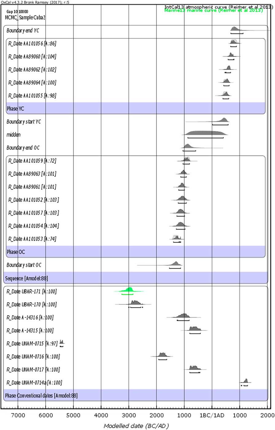
Figure 1 Chronology of the AMS 14C dates of Canímar Abajo and the 8 conventional 14C dates. Marginal posterior densities of all parameters included in the Bayesian modeling done with OxCal of the site of Canímar Abajo. Date “UBAR-171” correspond to the death of a shell. Hence, its date has been calibrated using the Marine 13 calibration curve.
The index agreement of the model is equal to 88 and the one of the overall agreement is equal to 87.1. The individual index agreement are given in Figure 1. The convergence of the Markov chain is checked and reached.
Figure 2 shows the plot of the marginal posterior densities of the start and the end of each burial activity. In addition, the time range of each burial activity is presented as well as the gap of time elapsed between them. Time range intervals are represented by a segment above the corresponding densities. The gap range is represented by a “two-dash” segment above the densities. Each interval is estimated with probability 95%.
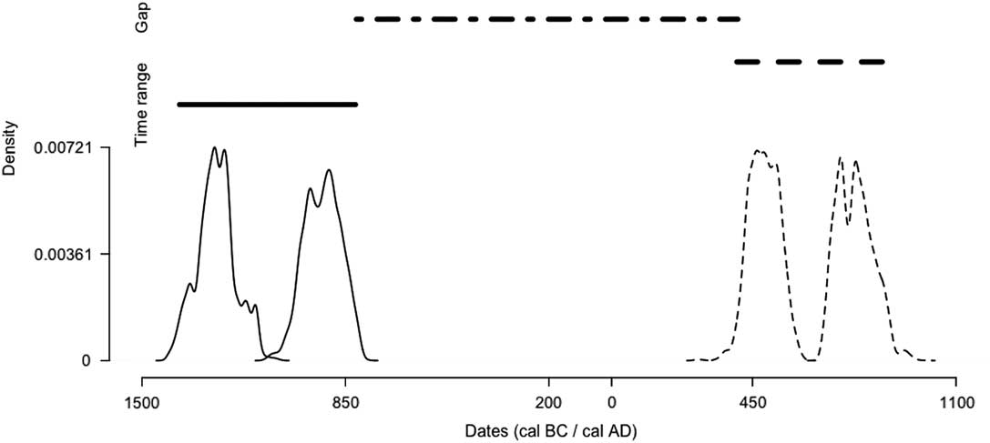
Figure 2 Chronology of the activities in the site of Canímar Abajo. While the densities of the beginning and the end of the Older Cemetery are drawn using solid lines, the densities of the beginning and the end of the Younger Cemetery are drawn using dashed lines. Segments above the densities correspond to the time range interval of the groups of dates associated to a level confidence of 95%. The “two-dash” segment corresponds to the gap range interval existing between both groups of dates associated to a level confidence of 95%. This graphic done with the R package ArchaeoPhases version 1.3.
Table 1 displays the numerical values of the intervals of interest: the HPD region of the start and the end of each burial activity, the time range interval of each burial activity, the HPD region of the “midden” date and the gap range interval. Each interval is given with probability 95%.
Table 1 Endpoints of HPD regions of each start and end parameters and of the “midden” date, endpoints of the Time range interval of both burial activities, and endpoints of the Gap range interval between both of them, Canímar Abajo, Cuba. (Results at level 95% obtained with ArchaeoPhases version 1.3).

From the stratigraphic information and the AMS 14C dates available in the site of Canímar Abajo, we can say that the activity of the OC started between 1514 cal BC and 1126 cal BC (HPD region at 95%) and ended between 1083 and 626 cal BC (HPD region at 95%). We can also defined the activity of the OC using a more compact tool, the time range interval that covers all the dates of the OC at 95%. According to this tool, the activity of the OC started at 1380 cal BC and ended at 818 cal BC with a probability of 95%. These two kinds of information are complementary. The time range interval is displayed together with the density of the start and end parameters of this group of dates in Figure 2.
The activity of the YC started between 65 cal AD and 695 cal AD (HPD region at 95%) and ended between 620 cal AD and 1120 cal AD (HPD region at 95%). In addition, we can summarize the activity of the YC by the time interval that covers all the dates of this cemetery at 95%. Using the time range interval, the activity of the YC started at 400 cal AD and ended at 893 cal AD with a probability of 95%. Again, these two kinds of information are complementary and are also displayed together in Figure 2. The “midden” date is associated with the following 95% HDP interval: 883 cal BC to 394 cal AD. We tested the existence of a gap between these two burial activities. The conclusion is that there is a gap between these two periods of activity from 815 cal BC to 403 cal AD at level 95%. This is probably the time during which the shell midden layer accumulated. This information is also displayed in Figure 2.
Analysis of the Eight Conventional 14C Dates
As the conventional dates were estimated on samples of bulked unidentified charcoal and extracted from contexts with bioturbation, we did not base the chronology of the site on these dates. Indeed, such dates have a potential for significant age-at-death offsets. However, we apply the testing procedure described herein to allocate the 8 conventional 14C dates to the most credible period among the five periods: before OC, OC, Midden period, YC, and after YC. Table 2 displays the probabilities that the conventional 14C dates belong to each period of the chronology. Dates are sorted according to their sampling level. The highest probability gives the most credible period for each date.
Table 2 Sampling information and posterior probability for the the 8 conventional 14C dates to belong to the periods of the chronology. Results are in %.

From Table 2, we can see that one date seems be more recent than the YC activity: the date of the sample UNAM.0714a. Indeed it has a probability of 100% to be in the period more recent than the YC. No dates belong to the YC. Two dates seem to belong to the Midden period with probability 100%: the dates of the sample UNAM.0717, the sample A.14315. A date seems to belong to the OC: the date of the sample A.14316. The four remaining dates belong to a period older than the OC with a probability of 100%: the dates of the sample UNAM.0716, the sample UNAM.0717, the sample UBAR.170 and the sample UBAR.171.
This analysis of the posterior densities shows that, except for two dates, the sampling level is in agreement with the chronology of the site. Indeed the sample A.14315 found deeper than the sample UNAM.0715 appears to be younger. Similar results are found for the sample A.14316 and the sample UBAR.170. We can see from the posterior densities, that only 3 samples were found in their related layer according to their 14C date. The 5 others were out of stratigraphic order if the chronology of the site is determined from the 12 AMS dates only. This is presumably due to bioturbation of the site and due to the context itself. Indeed as said by Roksandic et al.: “While stratigraphic superposition is a basic tool in archaeology for establishing relative chronology, interpretation is complicated in a burial context where younger burials may intrude into older layers.”
This analysis shows that the sampling level does not always give a good hint about the period of time to which a sample belongs. As a conclusion, to establish a chronology only dates from secure contexts should be used.
CONCLUSION
In this note we propose a fairly simple Bayesian model that takes into account the stratigraphy of the site of Canímar Abajo and 12 AMS 14C measurements. We implement this Bayesian modeling with OxCal. We then use the resulting joint posterior density in order to estimate the chronology of the site. To that aim, we analyze the highest posterior density regions of the start and end parameters of each mortuary activity and we apply complementary statistical tools: the time range intervals corresponding to the time period of the burial activities and a gap range interval corresponding to the hiatus between these two successive burial activities. These new tools, developed by Philippe and Vibet (Reference Guérin, Antoine, Schmidt, Goval, Hérisson, Jamet, Reyss, Shao, Philippe, Vibet and Bahain2017) and implemented in the R package “ArchaeoPhases” (see Philippe et al. Reference Philippe and Vibet2017), exploit the joint posterior distribution of collections of dates. These tools provide also potentially useful visuals for presenting chronologies.
Our analysis results in the estimation of the chronology of Canímar Abajo from the 12 14C dates from secure contexts and refines the results drawn by Roksandic et al. (Reference Reimer, Bard, Bayliss, Beck, Blackwell, Bronk Ramsey, Buck, Cheng, Edwards, Friedrich, Grootes, Guilderson, Haflidason, Hajdas, Hatté, Heaton, Hoffmann, Hogg, Hughen, Kaiser, Kromer, Manning, Niu, Reimer, Richards, Scott, Southon, Staff, Turney and van der Plicht2015). Indeed, they did not use a model and so reached approximate conclusions. From this Bayesian modeling, we can say that the activity of the OC started at 1380 cal BC and ended at 818 cal BC (with a probability of 95%), the activity of the YC started at 400 cal AD and ended at 893 cal AD (with a probability of 95%) and the midden shell layer seems to have been accumulated between 815 cal BC and 403 cal AD (with a probability at 95%).
For each conventional 14C date, we also estimate the most credible period among the five identified periods of the chronology, i.e., before OC, OC, Midden period, YC, and after YC. This analysis confirms the results drawn by Roksandic et al. (Reference Reimer, Bard, Bayliss, Beck, Blackwell, Bronk Ramsey, Buck, Cheng, Edwards, Friedrich, Grootes, Guilderson, Haflidason, Hajdas, Hatté, Heaton, Hoffmann, Hogg, Hughen, Kaiser, Kromer, Manning, Niu, Reimer, Richards, Scott, Southon, Staff, Turney and van der Plicht2015). It shows that in burial contexts, bioturbation may happen. Only identified samples extracted from a secure context should be used to establish a chronology.
In conclusion, we refine the chronology of Canímar Abajo by implementing a Bayesian modeling. The resulting chronology is similar to the one is described in Roksandic et al. (Reference Reimer, Bard, Bayliss, Beck, Blackwell, Bronk Ramsey, Buck, Cheng, Edwards, Friedrich, Grootes, Guilderson, Haflidason, Hajdas, Hatté, Heaton, Hoffmann, Hogg, Hughen, Kaiser, Kromer, Manning, Niu, Reimer, Richards, Scott, Southon, Staff, Turney and van der Plicht2015) based on simple inspection of calibrated dates. We used the statistical tools proposed in Philippe et al. (Reference Philippe and Vibet2017) in order to provide an estimation of the chronology of these two burial episodes, to test and to confirm the presence of a gap between them, and to estimate the length of time over which shell midden accumulated.
ACKNOWLEDGMENTS
The authors thank the editorial team and the referees for their relevant comments and useful suggestions, which helped us improve this article. The second author thanks the DefiMaths Program and Fédération de Recherche Mathématiques des Pays de Loire (France) for financial support.
APPENDIX
OxCal Script
Plot()
{
Curve("Atmospheric","IntCal13.14c");
Phase("Conventional dates")
{
R_Date("UNAM-0714a", 800, 50);
R_Date("UNAM-0717", 2520, 60);
R_Date("UNAM-0716", 3460, 60);
R_Date("UNAM-0715", 6460, 15);
R_Date("A-14315", 2515, 75);
R_Date("A-14316", 2845, 90);
R_Date("UBAR-170", 4200, 79);
Curve("Oceanic0","Marine13.14c");
R_Date("UBAR-171", 4700, 70);
};
Sequence()
{
Boundary("start OC");
Phase("OC")
{
R_Date("AA-101053", 3057, 39);
Curve("Oceanic1","Marine13.14c");
Delta_R("Local Marine OC",-108,30);
Mix_Curves("MixedOC","Atmospheric","Local Marine OC",30);
R_Date("AA-101054", 2999, 61);
R_Date("AA-101057", 2996, 53);
R_Date("AA-101052", 2946, 57);
R_Date("AA-89061", 2960, 33);
R_Date("AA-89063", 2922, 34);
R_Date("AA-101059", 2791, 51);
};
Boundary("end OC");
Date("midden");
Boundary("start YC");
Phase("YC")
{
Curve("Oceanic2","Marine13.14c");
Delta_R("Local Marine YC",-70,40);
Mix_Curves("MixedYC","Atmospheric","Local Marine YC",30);
R_Date("AA-101055", 1661, 52);
R_Date("AA-89064", 1617, 46);
R_Date("AA-89062", 1536, 51);
R_Date("AA-89060", 1420, 59);
R_Date("AA-101056", 1289, 46);
};
Boundary("end YC");
};
MCMC_Sample(Cuba2,10, 10000);
};


