INTRODUCTION
Understanding the outcome and manifestation of various climatic forces in the past at a regional level is a key issue in modern Quaternary research. Loess represents one of the most comprehensive semi-continuous paleoenvironmental records in the terrestrial zone (An et al. Reference An, Liu, Lu, Porter, Kukla, Wu and Hua1990; Pécsi Reference Pécsi1990; Pye Reference Pye1995; Lu and An Reference Lu and An1998; Kemp Reference Kemp2001; Porter Reference Porter2001, Reference Porter and Scott2007). It is also one of the most extensive types of Quaternary deposits, covering approximately 10% of the land surface (Pécsi Reference Pécsi1990; Pye Reference Pye1995).
The Madaras brickyard profile found in the northernmost fringe of the Bácska loess plateau is one of the thickest and best developed last glacial loess sequences in Hungary and Central Europe and spans the coldest period of the last glacial: The Last Glacial Maximum (LGM) (Sümegi Reference Sümegi2005; Hupuczi and Sümegi Reference Hupuczi and Sümegi2010; Bokhorst et al. Reference Bokhorst, Vandenberghe, Sümegi, Lanczont, Gerasimenko, Matviishina, Markovic and Frechen2011; Sümegi et al. Reference Sümegi, Gulyás, Csökmei, Molnár, Hambach, Stevens, Markovic and Almond2012) According to previously available 14C chronological data, the 10-m-thick profile of Madaras developed between ca. 29 and 12 kyr cal BP (Sümegi et al. Reference Sümegi, Gulyás, Csökmei, Molnár, Hambach, Stevens, Markovic and Almond2012). Following Woillard and Mook (Reference Woillard and Mook1982) and Vandenberghe (Reference Vandenberghe1985), this correspond to the time of the Middle and Late Pleniglacial on the European continent and MIS 2-1 (Lisiecki and Raymo Reference Lisiecki and Raymo2005).
This period has been characterized by numerous millennial-scale climatic fluctuations in the Northern Atlantic (Martinson et al. Reference Martinson, Pisias, Hays, Imbrie, Moore and Shackleton1987; Kreveld et al. Reference Kreveld, Sarnthein, Erlenkeuser, Grootes, Jung, Nadeau, Pflaumann and Voelker2000; Andersen et al. Reference Andersen, Svensson, Johnsen, Rasmussen, Bigler, Röthlisberger, Ruth, Siggaard-Andersen, Steffensen, Jensen and Vinther2006; Rasmussen et al. Reference Rasmussen, Andersen, Svensson, Steffensen, Vinther, Clausen, Siggaard-Andersen, Larsen, Dahl-Jensen, Bigler, Rhöthlisberger, Fischer, Hansson and Ruth2006; Svensson et al. Reference Svensson, Andersen, Bigler, Clausen, Dahl-Jensen, Davies, Sigfus, Muscheler, Rasussen, Rhöthlisberger, Steffensen and Vinther2006). Understanding how these were translated to the terrestrial realm and tackling potential leads and lags in regional responses to these climatic forcing requires the construction of reliable, independent time scales fostering comparison of marine and terrestrial records at high resolution. A comparison of our proxy results with other extra-regional records at the centennial scale requires the construction of reliable chronologies. As shown by Blaauw et al. (Reference Blaauw, Christen, Benett and Reimer2018), age-depth model choice, dating density and quality significantly affect the precision and accuracy of our chronologies. One date per millennium provides us millennial-scale precision. Precision can be improved by increasing dating densities on the one hand (Blaauw et al. Reference Blaauw, Christen, Benett and Reimer2018). However, there are cases when lack of sufficient funding hampers the inclusion of further dates in our analysis. In these cases, a comparison of the results of age-depth models can help us assess chronological precision (Blaauw et al. Reference Blaauw, Christen, Benett and Reimer2018). According to the findings of Blaauw et al. (Reference Blaauw, Christen, Benett and Reimer2018), classical age-depth models significantly underestimate uncertainty and are not improved in precision after a threshold in dating density is reached. On the other hand, Bayesian age-depth models relying on chronological ordering, as well as the fact that uncertainty is not constant between dated levels, reflecting our lack of knowledge for these depths, are more robust in providing realistic precision estimates (Blaauw et al. Reference Blaauw, Christen, Benett and Reimer2018). Although according to some, all age-depth models are wrong, but improving (Telford et al. Reference Telford, Heegaard and Birks2004; Trachsel and Telford Reference Trachsel and Telford2017) one should cook with what is available. Thus, assessing precision and accuracy of our models to make the best possible choice is inevitable in building chronologies. According to Blaauw et al. (Reference Blaauw, Christen, Benett and Reimer2018), a minimum of 2 dates per millennium is needed for achieving millennial-scale precision using Bayesian age-depth models. But what happens if this is not feasible?
In this paper we present the first independent time scale for the referred important paleoclimatic and paleoenvironmental record of Madaras. This time scale is based on 15 14C AMS dates, which span the entire 10 m profile with relatively even distribution (Figure 1). We aim to test the chronological precision of the age-depth models built, as well as their accuracy. The former can be done through statistics (via assessing uncertainty), while the latter is an arbitrary choice based on how well the model describes the observed sedimentological features of our profile (Blaauw et al. Reference Blaauw, Christen, Benett and Reimer2018). Finally, an attempt is made to see if the chosen model is “accurate” for our needs even if inclusion of further dates to improve precision is not possible due to certain reasons.
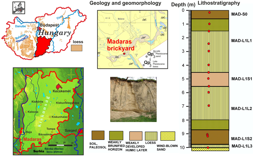
Figure 1 Location, lithostratigraphy of the studied loess/paleosol sequence of Madaras brickyard with sampling points for 14C AMS dating marked.
Location and Stratigraphy of the Loess/Paleosol Sequence of Madaras
The Madaras brickyard profile is located at 46°02′14.39″N and 19°17′15.01″E, at an elevation of 131.8 m asl (Figure 1). Based on sedimentological parameters, eight sedimentary layers were distinguished within the 10 m profile exposed (Sümegi Reference Sümegi2005; Sümegi et al. Reference Sümegi, Gulyás, Csökmei, Molnár, Hambach, Stevens, Markovic and Almond2012) (Figure 1). The bedrock of the profile is wind-blown sand overlain by a thin layer of yellowish-brown sandy loess (MAD L1L3). On top of the loess an intensively brunified paleosol layer (9.8–8.7 m) of pale brown hue (MAD L1S2) developed, embedding charcoal fragments of Scots pine identified via anthracological examinations and dated to the transition phase of the Middle and Late Pleniglacial (Table 1). This paleosol is capped by a weakly brunified horizon between the depths of 8.7–8.0 m. These deposits are overlain by yellowish brown moderately sorted coarse sandy silts (aeolian loess) up to the depth of 5.5 m (MAD L1L2) corresponding to the terminal part of the Middle Pleniglacial. On top of this loess a weak brunified soil of light pale brown color developed embedding carbonate nodules and smaller rhizoliths (MAD L1S1). This incipient soil is overlain by light yellow sandy loess of Late Pleniglacial age up to the depth of 1.5 m (MAD L1L1). From the depth of 1.5 m a weakly brunified zone was identified grading into the topmost modern soil. The topmost 0.6 m of the studied profile corresponds to the horizon of the modern soil (MAD-SO).
Table 1 Samples by type and depth as well as conventional 14C ages.
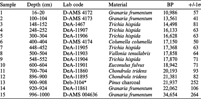
* Conventional GPC C-14 dating at Debrecen GPC Lab.
MATERIAL AND METHODS
14C Dating
One charcoal and 14 gastropod shell samples from the northern part of the loess wall were submitted for radiocarbon dating. AMS 14C dating measurements were performed in the AMS laboratory of Seattle, WA, USA (lab code D-AMS) and Institute for Nuclear Research of the Hungarian Academy of Sciences at Debrecen (lab code DeA-) (Table 1). The charcoal sample was measured by the Debrecen GPC Laboratory using conventional counting technique (Hertelendi et al Reference Hertelendi, Csongor, Záborszky, Molnár, Gál, Győrffy and Nagy1989). Certain herbivorous gastropods are known to yield reliable ages for dating deposits of the past 40 ka with minimal estimates of shell age offsets on the scale of perhaps a couple of decades (Újvári et al Reference Újvári, Molnár, Novothny, Páll-Gergely, Kovács and Várhegyi2014). This enables the construction of age models with resolution on the sub-centennial scale. (Sümegi and Hertelendi Reference Sümegi and Hertelendi1998; Pigati et al. Reference Pigati, Quade, Shanahan and Haynes2004, Reference Pigati, Rech and Nekola2010, Reference Pigati, McGeehin, Muhs and Bettis2013; Xu et al. Reference Xu, Gu, Han, Hao, Lu, Wang, Wu and Peng2011; Újvári et al. Reference Újvári, Molnár, Novothny, Páll-Gergely, Kovács and Várhegyi2014). Based on Hungarian studies by Sümegi and Hertelendi (Reference Sümegi and Hertelendi1998) and Újvári et al. (Reference Újvári, Molnár, Novothny, Páll-Gergely, Kovács and Várhegyi2014), sampled taxa were chosen accordingly (Table 1). Preparation of the samples and measurement followed the methods of Hertelendi et al. (Reference Hertelendi, Csongor, Záborszky, Molnár, Gál, Győrffy and Nagy1989 Reference Hertelendi, Sümegi and Szöőr1992) and Molnár et al. (Reference Molnár, Janovics, Major, Orsovszki, Gönczi, Veres, Leonard, Castle, Lange, Wacker, Hajdas and Jull2013). Shells were ultrasonically washed and dried at room temperature. Surficial contaminations and carbonate coatings were removed by pretreatment with weak acid etching (2% HCl) before CO2 production and graphitization. Conventional radiocarbon ages were converted to calendar ages using the software OxCal 4.2 (Bronk Ramsey Reference Bronk Ramsey2009) and the most recent IntCal13 calibration curve (Reimer et al. Reference Reimer, Bard, Bayliss, Beck, Blackwell, Bronk Ramsey, Buck, Cheng, Edwards, Friedrich, Grootes, Guilderson, Haflidason, Hajdas, Hatté, Heaton, Hoffmann, Hogg, Hughen, Kaiser, Kromer, Manning, Niu, Reimer, Richards, Scott, Southon, Staff, Turney and van der Plicht2013). Calibrated ages are reported as probability density ranges at the 2-sigma confidence level (95.4%).
Age-Depth Modeling
Taking into consideration the special pedogenetic processes and compaction during the deposition of loessy layers (Pécsi Reference Pécsi1990), the true sedimentation rate must have varied, and thus temporal resolution must have been different from cm to cm in our study profile (Pye Reference Pye1995). To count with these varying sediment accumulation rates several types of age-depth models have been applied for our dataset.
The first is the popular classical model of linear interpolation (Blaauw Reference Blaauw2010), which assumes that accumulation rates were constant between neighboring dated depths and changed, potentially abruptly, exactly at the dated depths (Bennett Reference Bennett1994; Blaauw and Heegaard Reference Blaauw, Heegaard, Birks, Juggins, Lotter and Smol2012). This model assumes a constant uncertainty between dated points, which contradicts of our lack of knowledge; i.e. higher uncertainty for these intervals. Then a classical polynomial model was also applied. All input data were from conventional 14C ages. Both the linear and polynomial models were built using the software Clam yielding us ages at every cm with 95% confidence intervals (CI). Sedimentation times (year/cm) with 95% CI was also calculated.
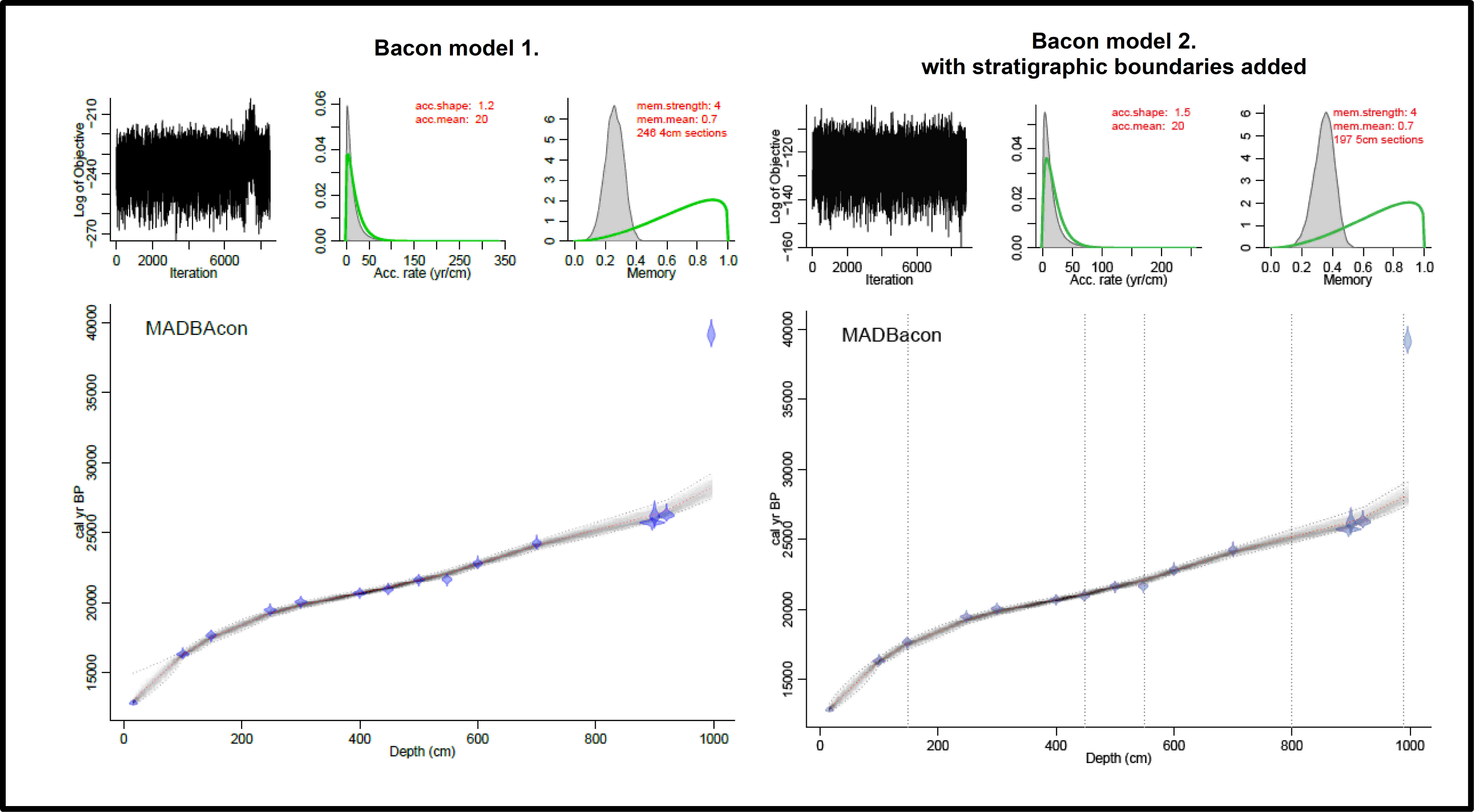
Bayesian modeling was performed using gamma and Poisson distributions as prior information on accumulation rates. Bacon (Blaauw and Christen Reference Blaauw and Christen2011) models the accumulation rates (AR) of many equally spaced depth sections based on an autoregressive process with gamma innovations. Inverse accumulation rates (sedimentation times expressed as year/cm) were estimated from 42 to 48 million Markov Chain Monte Carlo (MCMC) iterations, and these rates form the age-depth model. AR was first constraint by default prior information: acc. shape = 1.5 and acc. mean = 20 for the beta distribution, a memory mean = 0.7 and memory strength = 4 for beta distribution describing the autocorrelation of inverse AR. All input data were provided as 14C yr BP and the model used the northern hemisphere IntCal13 calibration curve (Reimer et al. Reference Reimer, Bard, Bayliss, Beck, Blackwell, Bronk Ramsey, Buck, Cheng, Edwards, Friedrich, Grootes, Guilderson, Haflidason, Hajdas, Hatté, Heaton, Hoffmann, Hogg, Hughen, Kaiser, Kromer, Manning, Niu, Reimer, Richards, Scott, Southon, Staff, Turney and van der Plicht2013) to convert conventional radiocarbon ages to calendar ages expressed as cal BP. Age modeling was run to achieve a 5-cm final resolution initially. In a second attempt to test the sensitivity of the model’s boundary conditions were added based on the observed major lithostratigraphic boundaries at the level of the modern soil (1.5 m), the weak middle paleosol (4.5–5.5 m) and the lowermost pedocomplex (8–9 m). In addition, the parameters were set as acc. shape = 2, 1.2 and acc. mean = 10, 20 for the gamma distribution and mem. mean = 0.4 and mem. strength = 10, 5, respectively. Model results with default prior information and new parameters as well as the adding of boundary conditions were compared. The fit of posterior gamma and beta distributions as well as the 95% CI ranges, plus inverse AR with 95% CI ranges were considered for comparing models. Finally, age-depth modeling was run using the set parameters. All data and figures are presented in calendar ages expressed as cal BP.
OxCal’s P_sequence (Bronk Ramsey Reference Bronk Ramsey2009) was tried with the granularity set to the size of the most dominant grain in the sequence (silt) (k = 0.3). Furthermore, to test the sensitivity, granularity (k) was also set to consider variable rates of sedimentation. In case of the latter, two sub-models were run: one without boundaries and one where stratigraphic boundaries have been introduced at 1.5, 4.5, 5.5, and 9.8 m, respectively. Ages were calculated for 1-cm intervals along with 95% CI to assess model uncertainty. Point estimates are based on the mean values.
The obtained ages of the different models (linear, polynomial, OxCal, Bacon) were evaluated for integrity and congruence as well as statistically significant differences using the non-parametric methods of pairwise Mann-Whitney U test for equality of medians and the Kolmogorov-Smirnov test for equality of distributions (Sokal and Rohlf Reference Sokal and Rohlf1995). In addition, mean 95% confidence ranges and maximum and minimum confidence values have also been calculated and compared to assess similarities and differences in uncertainty of ages (precision) for different parts of the profile. The fit of priors and posteriors in our Bayesian models was also a key to selecting the model with best chronological precision. These approaches however enabled us to test the chronological precision of the models alone (Blaauw et al. Reference Blaauw, Christen, Benett and Reimer2018). Accuracy was chosen according to the fit of the accumulation rates with our profile’s stratigraphic characteristics (Blaauw et al. Reference Blaauw, Christen, Benett and Reimer2018).
Sedimentation Rates
Sedimentation rates (mm/yr) are generally calculated using the equation
 $${\rm{AR}} = {{\rm{d}}_{2 - }}{{\rm{d}}_1}/{{\rm{a}}_{2 - }}{{\rm{a}}_1} \times 1000$$
where d1-2 are consecutive depths at 1-cm intervals and a1-2 are mean model ages. 95% confidence ranges are also calculated using the same equation but a1-2 here represents lower and upper 95% CI. This approach was adopted in our linear, polynomial and P-Sequence models. Despite its wide-range use (Újvári et al. Reference Újvári, Stevens, Molnár, Demény, Lambert, Varga, Timothy, Páll-Gergely, Buylaert and Kovács2017) the adoption of such equations may be suboptimal (Blaauw et al. Reference Blaauw, Christen, Benett and Reimer2018). Bacon however deals with variability in accumulation rates (sedimentation times in years/cm) through defining prior distributions. As such accumulation rates for any depth of the core are estimated by MCMC iterations providing more realistic views on precision and accuracy too (Blaauw and Heegaard Reference Blaauw, Heegaard, Birks, Juggins, Lotter and Smol2012; Blaauw et al. Reference Blaauw, Christen, Benett and Reimer2018).
Újvári et al. (Reference Újvári, Stevens, Molnár, Demény, Lambert, Varga, Timothy, Páll-Gergely, Buylaert and Kovács2017) reports sedimentation times for various Hungarian loess/paleosol profiles dated to MIS 2 and 3, including our study site as well. In their approach, Equation (1) is adopted in such way, that only the overall thickness of the profiles and the two boundary ages is used for the calculations. In our work sedimentation times with 95% CI were calculated using the accrate.depth.ghost function of Bacon for all depths at 1-cm intervals. This function allows to capture varying uncertainties with depth in contrast to Equation (1).
RESULTS
Age-Depth Models
Conventional radiocarbon ages for the studied depth intervals and material type are presented in Table 1. Relying upon the calibrated radiocarbon dates, the base sandy loess is dated to ca. 39 ka cal BP. The overlying loess-paleosol sequence of Madaras was formed between ca. 28 and 12 ka cal BP. Thus, the sequence captures the entire MIS 2 (Andersen et al. Reference Andersen, Svensson, Johnsen, Rasmussen, Bigler, Röthlisberger, Ruth, Siggaard-Andersen, Steffensen, Jensen and Vinther2006; Kreveld et al. Reference Kreveld, Sarnthein, Erlenkeuser, Grootes, Jung, Nadeau, Pflaumann and Voelker2000; Martinson et al. Reference Martinson, Pisias, Hays, Imbrie, Moore and Shackleton1987; Svensson et al. Reference Svensson, Andersen, Bigler, Clausen, Dahl-Jensen, Davies, Sigfus, Muscheler, Rasussen, Rhöthlisberger, Steffensen and Vinther2006) including the LGM as defined by Clark et al. (Reference Clark, Dyke, Shakun, Carlson, Clark, Wohlfahrt, Mitrovica, Hostetler and McCabe2009). Certain authors place the start of the LGM to different times (Denton et al. Reference Denton, Hausser, Lowell, Moreno, Andersen, Heusser, Schluchter and Marchant1999; Mix et al. Reference Mix, Bard and Schneider2001; Clark et al. Reference Clark, Dyke, Shakun, Carlson, Clark, Wohlfahrt, Mitrovica, Hostetler and McCabe2009). Based on available paleoecological data (Sümegi Reference Sümegi2005; Hupuczi and Sümegi Reference Hupuczi and Sümegi2010; Bokhorst et al. Reference Bokhorst, Vandenberghe, Sümegi, Lanczont, Gerasimenko, Matviishina, Markovic and Frechen2011; Sümegi et al. Reference Sümegi, Gulyás, Csökmei, Molnár, Hambach, Stevens, Markovic and Almond2012) it can be placed between 26,000–24,000 cal BP at our site. According to calibrated radiocarbon ages, the base of the profile starts between 39,807 and 38,590 cal BP (95.4%). The development of the first paleosol (MAD-L1S2) overlying the base sands (Figure 1) initiated between 26,570 and 26,009 cal BP years (95.4%) (Table S1). The topmost part of the sequence corresponding to the modern soil must be placed between 13,001 and 12,725 cal BP (Table S1); i.e. preceding the Pleistocene/Holocene transition. The 10-m profile thus spans ca. 16,000 years, rendering an overall average temporal resolution of 16 yr/cm.
Figure 2 presents the results of the linear fit, polynomial, P_Sequence (OxCal), Bacon 1 and 2 models with their 95% confidence ranges. All models display a similar trend. There is no significant difference between the point estimate mean ages of the individual models (see Tables 2, 3, S2). The average, minimum and maximum of mean 2σ error as well as 95% CI ranges of age estimate of the linear model (Table 2) is considerably lower than those of the polynomial and P_Sequence models. The average 2σ error is 192 years in contrast to the 404 years of the polynomial and 533 years of the P_Sequence models. The 95% CI range is 384 years with a minimum of 229 years at the depth of 18 cm and a maximum of 1187 years at the depth of 998 cm for the linear model (Table 2, Figure 2), where dates approach the maximum limit of 14C dating. The average 95% CI range of the polynomial model is much higher (686 years). The minimum value is nearly the same (246 years) to the previous model (Table 2). The maximum value of 1537 years is found at the bottom of the profile at the depth of 980 cm. Furthermore, while the second maximum value of 1490 years is found at the top, the minimum is located ca. 4 m below the top of the profile. Based on this observation regarding precision, the polynomial model can be excluded from our selection of age-depth model choices.

Figure 2 Comparison of constructed age-depth models (squares represent mean values of 14C dated horizons included in the model, solid lines represent mean values, dotted lines and whiskers correspond to 95% confidence intervals).
Table 2 Calendar dates received via simple calibration placed into linear, polynomial and P_Sequence (OxCal) models.

* Values based on 982 data at 1-cm intervals.
Table 3 Dates received for Bacon models 1. and 2. (without and with stratigraphic boundaries included) and differences in mean, mean 2σ error and 95% CI ranges.
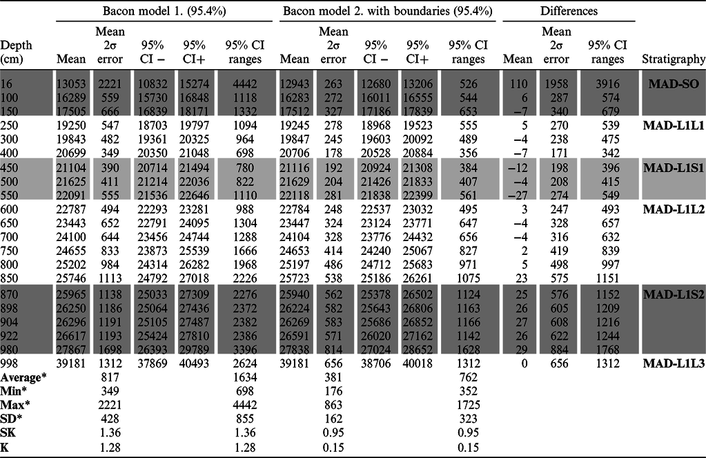
* Values based on 982 data at 1-cm intervals.
The average, minimum and maximum of 95% CI ranges of age estimate of the P_Sequence (OxCal) model (Table 2) is almost twofold of the values of the previous two models. So, the P_Sequence model is likewise less optimal in terms of chronological precision.
For Bacon models priors on accumulation rates (acc. shape:1.2 acc. mean: 20 year/cm) are very close to the posterior accumulation rates (Figure 2). Moderate (0.5–0.6) memory values indicate a somewhat variable rate of sediment accumulation, which is congruent with our understanding of dust deposition and loess formation (Figure 2). However, for Bacon model 1, both the average, minimum and maximum 2σ errors are higher than the P_Sequence and Bacon 2 models (Table 3). 95% CI is likewise wider for Bacon model 1 than the other two mentioned. In addition, the widest CI and 2σ error values are constrained to the uppermost and lowermost part of the sequence (Figure 2, Table 3). This is not the case for Bacon model 2. In this model the highest mean 2σ error and 95% confidence range values are confined to the bottom of the profile similarly to the P_Sequence model (Figure 2, Tables 2–3). However, the P_Sequence model could not handle ages properly beyond the depth of 9.22 m and yielded a simple linear interpolation with the calibrated date of the paleosol bedrock (MAD-L1L3) at the depth of 9.66 m (Figure 2) similarly to the linear and polynomial age-depth models. Bacon model 2, where a stratigraphic boundary has been introduced just above the bedrock could interpolate data down to this horizon (Figure 2, Table 3) implying that the deposition of the bedrock sands is much older than the overlying loess sequence. Differences in interpolated mean values between Bacon models 1 and 2 is negligible (Table 3) apart from the uppermost modern soil part, where both mean 2 σ error and 95% CI ranges are extremely high in model 1 (Figure 2, Table 2). Differences in mean age values between the two models is the minimal for the lower (MAD-L1L2) and upper (MAD-L1L1) loess packs (Table 3). The highest differences are noted for the lowermost paleosol horizon (MAD-L1S2), the modern soil (MAD-S0) as well as the weakly developed paleosol horizon (MAD-L1S1) intercalated between the older and younger loess packs. Mean 2σ error and 95% CI ranges are almost twofold in Bacon model 1 compared to Bacon model 2. When we compare the output of all models mean 2σ error and 95% CI ranges are the lowest in the linear and Bacon 2 models (Tables 2 and 3). These two models seem to have the highest chronological precision. But as previously stated, linear models tend to underestimate uncertainty (Blaauw et al. Reference Blaauw, Christen, Benett and Reimer2018). As Bacon models take into consideration the chronological ordering by providing a priori accumulation rates, comparing these with those of the model output can help us assess the “accuracy” of the model. As both the a priori and posterior accumulation rates are very similar in Bacon model 2 (Figures 2 and S1), this model seems to be ideal to realistically mimic sediment accumulation both in terms of precision and accuracy. This model is also the one that best captures the observed stratigraphy; i.e. most accurate.
To further assess the accuracy of the models, sedimentation times per depth profile were created for all age-depth models (Figures 3 and 4). Here all models seem to handle well the observed lithological changes of our profile with the exception of the polynomial model. Stepwise changes are comparable in the rest of the models. Yet both the linear and the P_sequence model does not handle sedimentation times correctly beyond the depth of 9 m (Figure 3), where a progressive aging of the lowermost paleosol unit is postulated towards the base sands. This is in high contrast with our understanding of site evolution seen from the lithostratigraphy. Both Bacon models presume a uniform start of loess deposition much later than the bedrock sand (Figures 2 and 4). This assumption seems more realistic than the others. In addition, the close resemblance of a priori and posterior accumulation times in both Bacon models further corroborates our choice of the most “precise and accurate” model (Bacon 2).

Figure 3 Comparison of calculated sedimentation times (yr/cm) of the linear, polynomial and P-Sequence age-depth models with the observed stratigraphy (red lines: mean values, grey and black lines: 95% confidence ranges). (Please see electronic version for color figures.)

Figure 4 Comparison of calculated sedimentation times (yr/cm) of the Bacon age-depth models with the observed stratigraphy (red dotted lines: mean values, grey dotted lines: 95% confidence ranges, grey shading: probabilities with darker values corresponding to higher probabilities).
Sedimentation Rates Compared to Other Coeval Sites of the Carpathian Basin
For the entire LPS of Madaras mean sedimentation time was 16.8 yr/cm (15–18 yr/cm 95% CI) based on mid-point estimates calculated for 1-cm intervals using Bacon model 2 (Figure 5). Compared to other records in the literature (Újvári et al. Reference Újvári, Stevens, Molnár, Demény, Lambert, Varga, Timothy, Páll-Gergely, Buylaert and Kovács2017) this is somewhat lower than the one at Dunaszekcső (13.3 yr/cm) spanning a period from ca. 36–23.4 kyr cal BP. It must be noted though that the age-span of the two profiles are only partially overlapping. Furthermore, the average resolution of 13.3 yr/cm published for Dunaszekcső was calculated from the overall thickness of the entire sequence and the bracketing calibrated 14C ages (Újvári et al. Reference Újvári, Stevens, Molnár, Demény, Lambert, Varga, Timothy, Páll-Gergely, Buylaert and Kovács2017). When mean values are recalculated using mid-point estimates for data presented for 1-cm intervals by Újvári et al. (Reference Újvári, Stevens, Molnár, Demény, Lambert, Varga, Timothy, Páll-Gergely, Buylaert and Kovács2017), there is an increase to 15.8 yr/cm. Using this data, the difference in sedimentation times between the two sites is negligible (1 yr). So, sampling intervals at 2 and 4 cm will likewise yield similar resolution of 32 and 65 years at Dunaszekcső and 33–68 years at our site of Madaras for the timespan of the entire profile. However, Újvári et. al (Reference Újvári, Stevens, Molnár, Demény, Lambert, Varga, Timothy, Páll-Gergely, Buylaert and Kovács2017) used Equation 1 for presenting sedimentation times and accumulation rates in their profile. Despite the adoption of Bacon in the construction of their age-depth model, no evaluation of chronological precision and accuracy of sedimentation times is presented in a way done in our work.
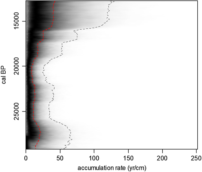
Figure 5 Calculated sedimentation times (yr/cm) against age using the Bacon 2 model (red dotted lines: mean values, grey dotted lines: 95% confidence ranges, grey shading: probabilities with darker values corresponding to higher probabilities).
For the period between 28 and 21 kyr, sedimentation times are quite similar along with the overall thickness of corresponding deposits at various sites of the Carpathian Basin (Table S3): Krems (14.5 yr/cm–4.7 m) (Lomax et al. Reference Lomax, Fuchs, Preusser and Fiebig2014), Süttő (18.3 yr/cm–3.45 m) (Novothny et al. Reference Novothny, Frechen, Horváth, Wacha and Rolf2011) Tokaj (12.2 yr/cm–4.6 m) (Schatz et al. Reference Schatz, Buylaert, Murray, Stevens and Scholten2012), Dunaszekcső (11.7 yr/cm–4.36 m) (Újvári et al. Reference Újvári, Stevens, Molnár, Demény, Lambert, Varga, Timothy, Páll-Gergely, Buylaert and Kovács2017), and our study site of Madaras (11.63 yr/cm–4.87 m) (Table S3). This implies relatively uniform conditions responsible for dust accumulation at first sight. However, for accurate evaluation temporal fluctuations should also be considered.
For the LGM part, which represents 70% of the entire LPS at Madaras, mean sedimentation time is even better: 11.63 yr/cm (11–12 cm/yr 95% CI) (Figure 6). Thus, sampling at intervals of 2 cm will yield us a resolution of ca. 23 yr per sample. 4 cm interval samples will still result in a sub-centennial resolution of 48 yr. Considering the total thickness of 6.8 m corresponding to the LGM (Figures 2 and 5), our study site seems to be the best resolved for the LGM in the Middle Danube region.
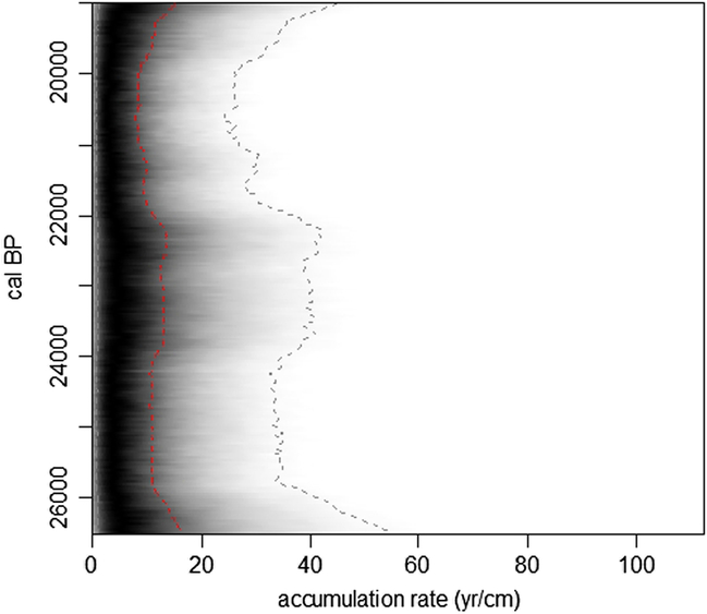
Figure 6 Calculated sedimentation times (yr/cm) against age using the Bacon 2 model for the period of the Last Glacial Maximum (red dotted lines: mean values, grey dotted lines: 95% confidence ranges, grey shading: probabilities with darker values corresponding to higher probabilities).
Average sedimentation rate (ASR) for the entire profile is 0.79 mm/yr (95% CI: 0.8–0.86 mm/yr) with the highest value of 1.43 mm/yr (95% CI: 1.33–1.54 mm/yr) recorded at 21.34 kyr cal BP based on mid-point estimates of the Bacon model 2 (Figures 5 and 6). This value is threefold of that presented by Újvári et al. (Reference Újvári, Kovács, Varga, Raucsik and Marković2010) (0.25 mm/yr) implying an unusually high dust accumulation at the site (average BMAR: 1183 g × cm–2 × kyr–1 95% CI: 849–1098 g × cm–2 × kyr–1). The highest recorded value of 2143 g × cm–2 × kyr–1 is confined to the nadir of the LGM. These new values are comparable to but somewhat lower than those recorded for the site of Dunaföldvár between 28.35 and 23.45 kyr b2k (1.002 mm/yr 95% CI: 1.132–1.34 mm/yr, 1504 g × cm–2 × kyr–1 95% CI: 1699–2024 g × cm–2 × kyr–1) (Újvári et al. Reference Újvári, Kovács, Varga, Raucsik and Marković2010 Reference Újvári, Stevens, Molnár, Demény, Lambert, Varga, Timothy, Páll-Gergely, Buylaert and Kovács2017). This site is found ca. 40–50 km to the west of our site. However, SR and BMAR values are significantly higher at Madaras for the period of the LGM, which represents 70% of the entire LPS: SR = 0.96 mm/yr 95% CI:0.95–1.01 yr/mm and BMAR = 1404 g × cm–2 × kyr–1 95% CI:1420–1516 g × cm–2 × kyr–1, respectively.
CONCLUSION
The 10-m loess/paleosol sequence of Madaras brickyard spans ca. 16 kyr of the latest phase of the last glacial. According to previous lithostratigraphic, sedimentological, chronological investigations (Sümegi et al. Reference Sümegi, Gulyás, Csökmei, Molnár, Hambach, Stevens, Markovic and Almond2012), the site was characterized by a strong variability of loess deposition and pedogenesis during the past ca. 28 ka cal BP. Dust accumulation and soil formation must have been in a highly fragile equilibrium mostly confined to the border zone during the formation of the entire sequence. Based on our findings Bacon model 2, including information on the visually identified stratigraphic boundaries, performed the best in achieving chronological precision for constructing a reliable chronology of the site. This model allowed for increased uncertainty between dated points, in light with our general understanding on lack of information but managed to constrain uncertainty to an acceptable level. It was also this model that most accurately captured the variability of sedimentation rates with varying uncertainties along the profile. This is a major advent in contrast to the use of generally accepted equations for calculating accumulation rates. The chosen model managed to mimic accumulation rates in terms of the observed stratigraphy and a priori determined sedimentation rates allowing for higher uncertainties at depths close to the bedrock and the modern soil.
The highest accumulation rates are put to the LGM, especially to its nadir. Newly calculated MAR and SR values are much higher than those published by Újvári et al. (Reference Újvári, Kovács, Varga, Raucsik and Marković2010) for the Carpathian Basin for the period of MIS 2. This must be an artefact of very few dates used by Újvári et al. (Reference Újvári, Kovács, Varga, Raucsik and Marković2010) on the one hand. Furthermore, in their work linear age-depth models without model and dating uncertainties have been adopted. A recently published work presents accumulation rates for the site of Dunaszekcső (Újvári et al. Reference Újvári, Stevens, Molnár, Demény, Lambert, Varga, Timothy, Páll-Gergely, Buylaert and Kovács2017) gained using Bayesian age-depth models in building a chronology. These are in the same range as those gained by our work. However, in contrast to our study, Újvári et al. (Reference Újvári, Stevens, Molnár, Demény, Lambert, Varga, Timothy, Páll-Gergely, Buylaert and Kovács2017) failed to use the sedimentation times yielded by the model itself to assess its “accuracy,” as accumulation rates are calculated using simple linear functions.
ACKNOWLEDGMENTS
Research has been carried out within the framework of University of Szeged, Interdisciplinary Excellence Centre, Institute of Geography and Earth Sciences, Long Environmental Changes Research Team. Support of Grants 20391-3/2018/FEKUSTRAT and GINOP-2.3.2-15-2016-00009 ‘ICER’ are acknowledged by the European Union and the State of Hungary, Ministry of Human Capacities, co-financed by the European Regional Development Fund.
SUPPLEMENTARY MATERIAL
To view supplementary material for this article, please visit https://doi.org/10.1017/RDC.2019.154