BACKGROUND

RESULTS AND COMPARISONS WITH OTHER DATASETS

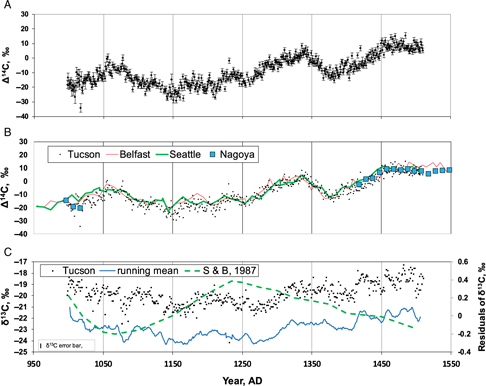
The data (supplementary Table S2) are presented as paired measurements of Δ¹⁴C and δ¹³C, and are depicted as a time-series of annual Δ¹⁴C and δ¹³C in Figure 1, where the data (referred to as the Tucson dataset below) are compared with (1) contemporaneous decadal data for Douglas fir samples, collected in the Pacific Northwest and measured at the University of Washington (the Seattle dataset: Stuiver and Becker Reference Stuiver and Becker1993; Stuiver et al. Reference Stuiver, Reimer and Braziunas1998), and (2) contemporaneous bidecadal data for Irish oak samples measured at Queen’s University, Northern Ireland (the Belfast dataset: Pearson et al. Reference Pearson, Pilcher, Baillie, Corbett and Qua1986; McCormac et al. Reference McCormac, Hogg, Higham, Lynch-Stieglitz, Broecker, Baillie, Palmer, Xiong, Pilcher and Brown1998). In Figure 2, the Tucson and Seattle annual datasets are combined with annual data (and some decadal data, or data averaged over decadal intervals, for clarity) from the Nagoya laboratory (Miyahara et al. Reference Miyahara, Masuda, Furuzawa, Menjo, Muraki, Kitagawa and Nakamura2004; Miyake et al. Reference Miyake, Nagaya, Masuda and Nakamura2012, Reference Miyake, Masuda and Nakamura2013a, Reference Miyake, Masuda and Nakamura2013b) to provide a record from AD 600 to 1953. Systematic differences exist between LSC Δ¹⁴C measurements from contemporaneous sets of tree rings from different continents, regardless of the laboratory that made the measurements (McCormac et al. Reference McCormac, Baillie, Pilcher and Kalin1995). An early evaluation based on non-corrected data from Seattle and Belfast and a partial Tucson dataset (Kalin et al. Reference Kalin, McCormac, Damon, Eastoe and Long1995) concluded that there was a satisfactory agreement between the Tucson and Seattle data, but noted a systematic offset between data from Tucson and Belfast. Damon et al. (Reference Damon, Eastoe, Hughes, Kalin, Long, Peristykh, Mook and van der Plicht1998) calculated a mean difference (non-corrected Seattle data minus Tucson data) of 1.0 ± 2.1‰ for decadal averages over the period AD 1065–1145, and concluded that the difference was well within error. Applying the same approach to the entire Tucson dataset and the corrected Seattle data, the average difference is 2.2 ± 3.2‰. The three datasets (Figure 1B) match in general, but show systematic differences over certain periods of several decades (Figure 3, for Seattle and Tucson data).

Figure 1 A. The Tucson Δ¹⁴C time series, with error bars (1σ). B. Comparison of the Tucson Δ¹⁴C time series (points) with the decadal Seattle and the decadal/bidecadal Belfast Δ¹⁴C time series (both represented as lines). C. The Tucson δ¹³C time series, with a 10-yr running mean displaced downward by 5‰. Also shown is the time series of average residuals of δ¹³C in a variety of North American tree species (Stuiver and Braziunas Reference Stuiver and Braziunas1987).

Figure 2 Annual and decadal Δ¹⁴C time series for tree rings since AD 600 (Tucson laboratory: this study; Seattle laboratory: Stuiver et al. Reference Stuiver, Reimer and Braziunas1998; Nagoya laboratory; some data expressed as decadal means: Miyahara et al. Reference Miyahara, Masuda, Furuzawa, Menjo, Muraki, Kitagawa and Nakamura2004; Miyake et al. Reference Miyake, Nagaya, Masuda and Nakamura2012, Reference Miyake, Masuda and Nakamura2013a, Reference Miyake, Masuda and Nakamura2013b), with a 3-yr running mean (displaced downwards by 12‰) for AD 998–1954. Named Grand Solar Minima and Maxima are shown. E(L)MSM = Early (Late) Medieval Solar Maximum, MOD SM = Modern Solar Maximum.

Figure 3 Time series of differences between the Seattle decadal dataset of Δ¹⁴C and the Tucson dataset expressed as decadal averages (Seattle minus Tucson), compared with a 10-yr running mean (rm) of the Tucson Δ¹⁴C time series.

For the Seattle measurements, each of which represents a single, high-precision decadal measurement, the typical standard deviation (1σ) is 2.5‰. For the decadal means calculated from the Tucson dataset, values of σ are calculated as standard errors of each decadal mean of Δ¹⁴C (supplementary Table S3). The typical value of σ for the difference (Seattle-Tucson) is between 2.6 and 2.9 ‰ (Table S3). The range of the decadal differences in Figure 3 is 14‰.

If the differences arose from measurement error only, their scatter as a function of time would be random. Such is not the case; whether the differences are depicted as individual points or moving averages, there appears to be a cyclic change in the magnitude of the differences, and the change is inversely related to the decadal means for the Tucson data (Figure 3). The cyclic variation of difference between the two datasets appears to be real, in that the extremes of difference are statistically different. Comparing the extended Tucson dataset with the Seattle decadal data suggests that systematic, cyclic differences, possibly climatic in origin, exist between the Pacific Northwest and the Sierra Nevada. The Tucson δ¹³C time-series (Figure 1C) shows a long-term change broadly matching that of the Δ¹⁴C data, and shorter cyclic variations.

SPECTRAL ANALYSIS

The data in the vicinity of the Late Medieval Solar Maximum have been detrended by (1) calculation of a smoothing spline for T = 200 yr (Figure 4) which has the effect of removing cyclic variations of T/2 or less, and (2) subtraction of the spline from the dataset, leaving the short-period cycles without long-term trends (Figure 5). A period near 55 yr is clearly seen, along with cycles with T near 10 yr. This shorter cycle has intervals of low amplitude near AD 1130 and 1240, suggesting amplitude modulation with T near 110 yr.

Figure 4 Δ¹⁴C data for the Late Medieval Solar Maximum: Tucson dataset, annual data (points) with a smoothing spline (line) with gain 0.95 and a period of 200 yr.

Figure 5 Δ¹⁴C data for the Late Medieval Solar Maximum: Tucson dataset, annual data, detrended by subtraction of the smoothing spline in Figure 4.

Discrete Fourier Transformation (DFT) of the detrended data (modified by subtraction of the smoothing spline for T= 200 yr) shows strongest peaks at 126, 91, 56, 17.6, 13.6, 10.4, and 7.1 yr (Figure 6). Amplitudes < 0.5 units appear to be noise; only peaks of greater amplitude are labeled with the corresponding period in years. Periods less than 5 yr are probably spurious.

Figure 6 Discrete Fourier Transform power spectrum of the detrended Tucson Δ¹⁴C dataset. Larger peaks are labeled with the corresponding period in years.

The distribution of short-T variations in time can be seen in the spectrogram (Figure 7) constructed using a 77-yr moving window. Periods near 7 yr are most in evidence during the interval AD 1320–1450. Periods of 10–17 yr are most prominent during the interval AD 1000–1120. A 56-yr period persists between AD 1000 and 1200 and from 1350 to 1400, but is weak or absent at other times.

Figure 7 Spectrogram of Tucson Δ¹⁴C data (frequency vs. time plot showing contours of Discrete Fourier Transform spectral amplitude for a 77-yr time window). Yellow and enclosed colors indicate high amplitudes. Horizontal dashed lines mark prominent periods.

COMPARISON WITH ANNUAL DATA, AD 1510–1954

Considering cyclicities between the 88-yr Gleissberg cycle and 5 yr, Stuiver and Braziunas (Reference Stuiver and Braziunas1993) noted periods of 56, 26, 17, 13.2, 10.4, 6.4, 5.7, and 5.1 yr in the Seattle annual dataset for AD 1510–1954. This set of periods compares closely with the Tucson power spectrum for T > 5 yr. As discussed above, the Seattle and Tucson laboratories produce data that appear to be comparable in accuracy and precision, but the raw Tucson data in Figure 2 appear to show greater scatter than the Seattle data. Whether this arises from the raw material or from experimental technique is unclear. If there were greater scatter due to error in the Tucson data, however, the error should be random and would be attenuated by smoothing. Figure 2 shows that smoothing in fact results in the detection of non-random cyclic variations in both datasets. The cycles are the 7–17-yr periods described above, and their amplitude, particularly between AD 1000 and 1300, is larger than that of corresponding periods in the Seattle data. Outlying results (supplementary Table S2), present in the Tucson dataset to a greater degree than in the Seattle dataset, include five large jumps in Δ¹⁴C at AD 1017 (negative jump, AMS measurement), AD 1160 (negative, LSC), AD 1165 (negative, LSC), AD 1231 (positive, LSC), and AD 1420 (positive, LSC). Laboratory contamination might be expected to shift δ¹³C either positively (atmospheric contamination) or negatively (contamination from pre-treatment chemicals); however, only the outlier at AD 1231 has a δ¹³C value markedly different from neighboring data. Large jumps in Δ¹⁴C are present in comparable datasets (Miyahara et al. Reference Miyahara, Masuda, Furuzawa, Menjo, Muraki, Kitagawa and Nakamura2004, Reference Miyahara, Yokoyama, Yamaguchi, Kosovichev, Andrei and Rozelot2009; Miyake et al. Reference Miyake, Nagaya, Masuda and Nakamura2012). Whether the outliers in the Tucson dataset result from experimental shortcomings or from the nature of the raw samples remains unclear. The data are presented here without censoring.

SHORT-TERM EVENTS

Annual time-series data are of use in identifying decadal cyclic phenomena such as the Schwabe and Hale cycles of solar activity, and non-cyclic phenomena of similar time-scale, for example the generation of ¹⁴C pulses by SPEs from large solar flares. The cyclic phenomena are expected to approximate sinusoids, while the non-cyclic events may appear as abrupt single-year changes followed by slower reversal of the initial change, approximating a single cycle of a square wave. The latter are termed stepwise changes below.

Stepwise Events

The AD 1006 SN, observed optically, may have produced the stepwise increase in Δ¹⁴C of about 8.5‰ at AD 1010–1011 in our time-series of Δ¹⁴C (Damon et al. Reference Damon, Dai, Kocharov, Mikheeva, Peristykh, Cook, Harkness, Miller and Scott1995a, Reference Damon, Kocharov, Peristykh, Mikheeva and Dai1995b), followed by gradual decay over a decade. The delay between the arrival of visible light and gamma radiation may have resulted from a delay in the arrival of gamma rays relative to visible light (Damon et al. Reference Damon, Dai, Kocharov, Mikheeva, Peristykh, Cook, Harkness, Miller and Scott1995a, Reference Damon, Kocharov, Peristykh, Mikheeva and Dai1995b), but may be partly explained by phase shift due to low-pass filtering. If this pulse of radiation is considered as a square wave of period 12 yr, its principal sinusoidal component also has a period of 12 yr, with a phase shift of about 2 yr and an attenuation factor comparable to that for T ≈ 10 yr. Dee et al. (Reference Dee, Pope, Miles, Manning and Miyake2017), however, discounted a SN as the cause of the stepwise increase because tree-ring records from other localities fail to show what should have been a global phenomenon.

Both Damon et al. (Reference Damon, Dai, Kocharov, Mikheeva, Peristykh, Cook, Harkness, Miller and Scott1995a, Reference Damon, Kocharov, Peristykh, Mikheeva and Dai1995b) and Miyake at al. (Reference Miyake, Nagaya, Masuda and Nakamura2012) considered SPEs arising from clusters of giant solar flares as an alternative explanation for stepwise increases in Δ¹⁴C. However, Damon et al. (Reference Damon, Dai, Kocharov, Mikheeva, Peristykh, Cook, Harkness, Miller and Scott1995a, Reference Damon, Kocharov, Peristykh, Mikheeva and Dai1995b) concluded that Δ¹⁴C signatures of clusters of flares of the required energy are absent in the Seattle dataset between AD 1500 and 1954 (Stuiver and Braziunas Reference Stuiver and Braziunas1993), and that such SPEs would therefore be unlikely at earlier times.

Additional stepwise increases in Δ¹⁴C, all ≤ 5‰, may be present in the Tucson dataset (supplementary Figure S1 and Table S2) at AD 1063, 1167, 1297, 1429, and 1448–1450. Possible stepwise decreases are less common, at AD 1182 and 1367, both about 5‰. All of these changes are comparable in amplitude to the Schwabe-like cycles, and therefore difficult to distinguish reliably.

Usoskin and Kovaltsov (Reference Usoskin and Kovaltsov2012) suggested large SPEs dated approximately at AD 1460 and 1505 on the basis of ¹⁰Be data from an ice core at the South Pole. The stepwise change at AD 1448–1450 in the Tucson Δ¹⁴C record (Figure 8) is 4.9‰, calculated as the difference between means for the preceding and following time intervals indicated by horizontal bars. The change coexists with a 5-yr decrease of about 0.6‰ in δ¹³C, which may indicate a climate effect corresponding to the change in Δ¹⁴C. We suggest that these stepwise changes correspond to the AD 1460 SPE, with better time resolution. A 5‰ stepwise change also appears to be present near AD 1450 in the Δ¹⁴C record of Miyahara et al. (Reference Miyahara, Masuda, Muraki, Kitagawa and Nakamura2006). At AD 1506–1507 in the Tucson dataset (Figure S1), a series of declining Δ¹⁴C values is abruptly interrupted by a 6‰ increase that is difficult to distinguish in form from neighboring Schwabe-like cycles (Figure S1).

Figure 8 Tucson Δ¹⁴C data, AD 1378–1472 (continuous curve), detrended using the linear regression shown (diamond symbols), compared with the Tucson δ¹³C time series. Solid bars indicate mean Δ¹⁴C and δ¹³C (over the intervals indicated by bar length, with standard errors, se, indicated) around the 4.9‰ change in Δ¹⁴C at AD 1450.

A very large volcanic eruption that occurred in AD 1258 or 1259 (Emile-Geay et al. Reference Emile-Geay, Seager, Cane, Cook and Haug2008) is not convincingly recorded in the Tucson Δ¹⁴C and δ¹³C records (supplementary Figure S1), but corresponds to a decade, beginning in AD 1256, of thin tree rings (supplementary Table S2).

THE δ¹³C RECORD

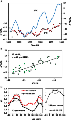
The time-series of δ¹³C and Δ¹⁴C are broadly similar in form (Figures 1A ,1C, 9A). The δ¹³C and Δ¹⁴C time series, expressed as decadal averages in order to eliminate short-period noise, are most closely related in the interval AD 1100–1510, within which R² = 0.69 (Figure 9B). For the entire dataset, AD 998–1510, R² = 0.53, reflecting poor correlation in the interval AD 998–1100. The R² values have been calculated for decadal averages, beginning AD 1105, 1115 etc. (see Table S1); note that the values of R² are lower when calculated for decades beginning AD 1100, 1110, etc., e.g. 0.63 for AD 1100–1510. For both sets of decadal means, R² is maximized if δ¹³C lags behind Δ¹⁴C by 10 to 30 yr, or 130 to 140 yr (Figure 9C). This lag appears to be related to cycles with T near 110 yr in both datasets, causing R² to have a second maximum where the cycles realign with increasing applied lag. Lag between δ¹³C and Δ¹⁴C at millennial time scale is more difficult to determine in a dataset spanning 513 yr; using 100-yr means calculated every 25 yr (in order to remove short-period variations) suggests that R² is maximized if δ¹³C lags behind Δ¹⁴C by 25–50 yr (Figure 9C).

Figure 9 A. Time-series plot of decadal averages of Δ¹⁴C and δ¹³C for the Tucson dataset. B. Δ¹⁴C vs. δ¹³C, for AD 1100–1510; the points represent decadal averages, beginning AD 1105, 1115 etc. (see Table S3); the value of R² is lower for decades beginning AD 1100, 1110, etc. C. Effect of time lag on correlation (R²) of Δ¹⁴C vs. δ¹³C for decadal means, with separate calculations for AD 1100–1510 and AD 998–1510 (left), and for 100-yr means, calculated every 25 yr for AD 998–1510 (right). A positive lag signifies δ¹³C lagging behind Δ¹⁴C. R² values within dashed ellipses have p values < 0.0001.

The changes in δ¹³C reflect surface environmental factors, not the cosmogenic processes ultimately responsible for the Δ¹⁴C time series. Carbon isotope discrimination between a C₃ plant (p) and air (a) is

$${\Delta _{\rm{3}}} &#x003D; {{\delta (a) - \delta (\,p)} \over {1 + 0.001\delta (\,p)}} \approx \delta (a) - \delta (\,p)$$(1)

(Farquhar and Richards Reference Farquhar and Richards1984) where the δ symbols (simplified to δ_p and δ_a below) denote δ¹³C. Values of δ_a have remained close to constant in the global atmosphere over the time interval AD 1000–1500, on the evidence of measurements in ice cores (e.g. Rubino et al. Reference Rubino, Etheridge, Trudinger, Allison, Battle, Langenfelds, Steele, Curran, Bender and White2013). Persistent local inhomogeneities of 1‰ or more in δ_a are unlikely at annual to decadal time scales and have not been observed in recent decades (Carbon Dioxide Information Analysis Center 2010). Values of δ_p are therefore inversely related to values of Δ₃.

Relevant environmental variables at the study site include temperature, water availability (encompassing both relative humidity of air and availability of soil water) and irradiance (Farquhar et al. Reference Farquhar, Ehleringer and Hubick1989; McCarroll and Loader Reference McCarroll and Loader2004; Cernusak et al. Reference Cernusak, Ubierna, Winter, Holtum, Marshall and Farquhar2013). Observed δ_p values result from the complex interplay of two biological functions: stomatal conductance, mediated by water availability, and photosynthetic rate, controlled by temperature and irradiance. Where plants are not subjected to extremes of stress from heat and dryness (as in the present study area), it is not possible to determine a simple causality for variations in δ_p (McCarroll and Loader Reference McCarroll and Loader2004, and references therein). Nonetheless, three of the four variables are climatic in origin; the origin of the fourth, irradiance, is discussed below. Even though a positive correlation between Δ₃ and ambient temperature has been suggested from studies of lowland plants from various latitudes (Körner et al. Reference Körner, Farquhar and Wong1991), and in individual plants (e.g., Leavitt and Long Reference Leavitt and Long1982), contrary results exist (McCarroll and Loader Reference McCarroll and Loader2004). Likewise, although a global positive correlation has been suggested between Δ₃ and mean annual precipitation (Diefendorf et al. Reference Diefendorf, Mueller, Wing, Koch and Freeman2010) and in individual trees (e.g. Leavitt and Long Reference Leavitt and Long1991), studies reviewed by McCarroll and Loader (Reference McCarroll and Loader2004) indicate a complex dependence.

Irradiance correlates negatively with Δ₃ (Ehleringer et al. Reference Ehleringer, Field, Lin and Kuo1986; Leavitt and Long Reference Leavitt and Long1991). Ehleringer et al. (Reference Ehleringer, Field, Lin and Kuo1986) observed decreases of about 4‰ in δ_p where irradiance was reduced by a factor of 2.3 because of shading. Annual solar irradiance changes by 6% owing to the elliptical geometry of the Earth’s orbit (Floyd et al. Reference Floyd, Tobiska and Cebula2002), and by a factor of 2 (neglecting absorption in the atmosphere) at 37ºN as a result of seasonal change in the incident angle of solar radiation. The Schwabe cycle produces changes in solar irradiance in the visible spectrum that are much smaller, 0.1–0.38%, (Hoyt and Schatten Reference Hoyt and Schatten1997, p. 196 ff.). Change in visible irradiance between the Maunder Minimum and the present is likely to be of similar magnitude (Lean Reference Lean2000). Photosynthetic effects of solar luminosity cycles are therefore small relative to those arising from shorter-term phenomena, and are unlikely to cause large changes in δ_p.

The effect of irradiance (governed by the amount of shading from tree canopies), combined with the effects of tree height on the availability of water in leaf tissue (governed by hydraulic conductivity in tree trunks) causes Δ₃ to decrease with tree height (Leavitt Reference Leavitt2010; McDowell et al. Reference McDowell, Bond, Dickman, Ryan, Whitehead, Meinzer, Lachenbruch and Dawson2011). Ambrose et al. (Reference Ambrose, Sillett and Dawson2009) measured the effect in leaves of contemporaneous individuals of Sequoiadendron giganteum, finding that Δ₃ decreased by 3–4‰ as tree height increased from 30 to 90 m, which can be compared with our observed increase of 3 to 3.5‰ in δ¹³C of cellulose between AD 1150 and 1490 (Figure 1B). Most height-growth in sequoias takes place in the first 400 yr, but trunk volume continues to increase steadily until an age of at least 2500 yr in the case of the General Sherman tree (Weatherspoon Reference Weatherspoon, Bums and Honkala1990). Craig (Reference Craig1954) recorded an increase of 2‰ in δ¹³C during the first 200 yr of growth of a sequoia, and little change in the succeeding 600 yr. The age of the tree sampled for this study was not noted by the samplers. However, the sampling of broader rings since AD 1024 probably represents the later phase of growth, with modest increase in height and thus little change in δ¹³C attributable to tree growth.

Two possible explanations of the long-term changes in our δ¹³C time series arise: (1) that the long-term increase in δ¹³C is a consequence of growth of the tree, with secondary cyclic variations resulting from changes in environmental factors; and (2) that changes in δ¹³C arise from the factors controlling Δ¹⁴C, i.e. that solar luminosity was modulating climate at the Big Stump Grove in such a way as to generate long-term trends in δ¹³C. If (1) is correct, then the long-term parallel changes in δ¹³C and Δ¹⁴C in the Tucson dataset (Figures 1B, 9A) are coincidental. Our dataset shows a general decrease in δ¹³C between AD 998 and AD 1150, inconsistent with the δ¹³C change expected in early growth of a tree. This and the shared variance of δ¹³C and Δ¹⁴C favor explanation (2), notwithstanding our inability to identify causality in detail.

A complex interplay of environmental variables seems likely to be related to the noise in the annual δ¹³C record (Figure 1C), and also to the lack of correspondence between the sequoia δ¹³C record and dendrochronological records from the immediate region (Hughes and Brown Reference Hughes and Brown1992; Graumlich Reference Graumlich1993; Scuderi Reference Scuderi1993; Figure S2). Our sequoia δ¹³C time series also bears no relationship (Figure 1B) to δ¹³C in tree rings for multiple species at other locations over the same time interval (Stuiver and Braziunas Reference Stuiver and Braziunas1987). The latter data are expressed as residuals of δ¹³C (the differences between decadal δ¹³C measurements and the pre-1850 mean δ¹³C for each species) and have a range of 1.2‰, smaller than δ¹³C ranges found in the Tucson dataset, namely 3.3‰ in decadal averages and 5.2‰ in annual measurements (Table S2, excluding a single outlier).

DISCUSSION: IMPLICATIONS FOR CLIMATE CHANGE

The δ¹³C time series does not meet usual dendrochronological standards in that it is derived from a single tree. It is noisy, no doubt owing to short-term changes in environmental parameters (see previous section). Nonetheless, the time-series of Δ¹⁴C and δ¹³C in this study are strikingly similar in form with and without low-pass filtering (Figures 1 and 9A). The δ¹³C signal—a change of 3.5‰ in the smoothed δ¹³C time series—is large in the context of tree-ring isotope data (e.g. Körner et al. Reference Körner, Farquhar and Wong1991; Leavitt and Long Reference Leavitt and Long1991; Leavitt Reference Leavitt2010).

The Δ¹⁴C time series provides a record originating as changes in cosmogenic production rates of ¹⁴C and is attenuated and phase-shifted as described above (Background). The δ¹³C time series provides a record of long-term change in multiple interacting environmental parameters. The long-term δ¹³C record is therefore probably best explained as a product of climate change, the details of which cannot be deduced from δ¹³C alone. The principal mode of variation of the Δ¹⁴C and δ¹³C time series in this study is part of a cycle with a period (T) of 850 to 1000 yr (Figure 2). A secondary cyclicity with T near 100 yr is also visible in both series.

A recent version of the dependence of ¹⁴C phase shift on T (Beer et al. Reference Beer, McCracken and von Steiger2012, Figure 13.5.3.2-2) gives lags of 100–125 yr for T = 1000 yr between extrema of production of ¹⁴C in the upper atmosphere (inversely related to extrema of solar luminosity) and subsequent, corresponding extrema archived at Earth’s surface. For T = 100 yr, the lag is 10 yr. Earlier versions (Damon and Peristykh Reference Damon and Peristykh2004; Usoskin and Kromer Reference Usoskin and Kromer2005) gave lags of 60–110 and 19–21 yr, respectively. The smoothed δ¹³C time series expressed as 10-yr means (Figure 9A), lags behind the Δ¹⁴C time series by 10 to 30 yr (Figure 9C). As explained above, this additional lag applies to the centennial cyclicity. For the millennial cycle of δ¹³C, an additional lag of 25–50 yr is suggested (Figure 9C). The Tucson dataset therefore indicates a lag (incorporating the phase-shift estimate of Beer et al. Reference Beer, McCracken and von Steiger2012) of 20–40 yr between extrema of the centennial cycles of solar luminosity and δ¹³C, an effect seen most clearly between AD 1100 and 1500. Less clearly, there appears to be a lag of 125–175 yr between extrema of the millennial cycles of solar luminosity and δ¹³C.

Helama et al. (Reference Helama, Fauria, Mielikainen, Timonen and Eronen2010), in a study comparing widths of tree rings from Arctic Scandinavia and reconstructed sunspot numbers over the past 2000 yr, concluded that the millennial component of their tree-ring data lagged behind that of reconstructed sunspot numbers by 70–100 yr for the Late Holocene. If the long-term δ¹³C signal in our dataset is indeed of climatic origin, then a similar, but larger, lag of climate behind solar luminosity is implied, regardless of whether we can identify the specific cause of the long-term change in δ¹³C. A similar lag of 20–40 yr for the centennial component is implied. The studies describe regional effects, in widely separated regions of contrasting climate. Both studies assume that the phase shifts calculated from models of the carbon cycle are correct.

The most recent grand solar maximum occurred between AD 1960 and 1980, according to sunspot numbers (e.g. SILSO, 2019). It is not yet clear whether this maximum represents the culmination of the millennial cycle or a maximum of the centennial cyclicity superimposed on the millennial cycle, in which case the post-1980 decrease in sunspot numbers would be analogous to the punctuation of the long Medieval Solar Maximum by the Oort minimum (Figure 2). Steinhilber and Beer (Reference Steinhilber and Beer2013) deduced that the millennial grand maximum had occurred late in the 20th century, whereas Damon and Peristykh (Reference Damon and Peristykh2005) forecast it for about AD 2040. If the AD 1960–1980 grand maximum is of millennial time-scale, the corresponding peak climatic response, which may be more complex than warming alone, is predicted to lag behind the sunspot and luminosity maxima by at least a century, therefore occurring in the second half of the 21st century. This study suggests that peak climatic response to a centennial AD 1960–1980 grand maximum would end before AD 2020, but that the response to the underlying millennial component of increasing solar luminosity would continue into and possibly beyond the second half of the 21st century.

Predicting the magnitude of such climate response in relation to that arising from greenhouse gases is not straightforward. Two contrasting opinions are present in the literature. According to the first, the influence of solar activity is miniscule in comparison to the effect of anthropogenic greenhouse gases. Myhre et al. (Reference Myhre, Shindell, Bréon, Collins, Fuglestvedt, Huang, Koch, Lamarque, Lee, Mendoza, Stocker, Qin, Plattner, Tignor, Allen, Boschung, Nauels, Xia, Bex and Midgley2013) and Masson-Delmotte et al. (Reference Masson-Delmotte, Schulz, Abe-Ouchi, Beer, Ganopolski, González Rouco, Jansen, Lambeck, Luterbacher, Naish, Stocker, Qin, Plattner, Tignor, Allen, Boschung, Nauels, Xia, Bex and Midgley2013) in their reviews for the Intergovernmental Panel on Climate Change (IPCC) concluded that the radiative forcing attributable to changes in total solar irradiance (TSI) is small during Schwabe cycles, less than 1% of the radiative forcing due to greenhouse gases. That claim appears to be based on satellite measurements of TSI, modeled estimates of anthropogenic effects, and temperature observations during recent solar cycles. The authors suggested further that the amplitude of cyclic variations in TSI due to the Schwabe cycle is approximately the same as that due to the transition from the Maunder minimum to the modern grand solar maximum. The magnitude of the latter is less certain than that of the former.

According to the second opinion, the component of climate change due to solar radiative forcing is larger than that corresponding to the IPCC opinion. Direct observation and climate proxy archives show clear evidence of changes due to solar luminosity cycles at the time scale of the Schwabe cycle (e.g. Rigozo et al. Reference Rigozo, Nordemann, Evangelista da Silva, de Souza Echer and Echer2007; Meehl et al. Reference Meehl, Arblaster, Matthes, Sassi and van Loon2009; Perone et al. Reference Perone, Lombardi, Marchetti, Tognetti and Lasserre2016) and at longer time scales (e.g. Mann et al. Reference Mann, Bradley and Hughes1998; Yu and Ito Reference Yu and Ito1999; Eichler et al. Reference Eichler, Olivier, Henderson, Laube, Beer, Papina, Gäggeler and Schwikowski2009; Beer et al. Reference Beer, McCracken and von Steiger2012, Figure 17.5–2; Soon et al. Reference Soon, Connolly and Connolly2015). Damon and Peristykh (Reference Damon and Peristykh2005) estimated that 18% of 20th-century global warming was attributable to solar forcing. Possible mechanisms may involve (1) heating of the troposphere and upper stratosphere as a result of the formation and destruction of ozone by incident ultraviolet radiation (Hoyt and Schatten Reference Hoyt and Schatten1997; Meijer et al. Reference Meijer, Dergachev, van der Plicht, Renssen, Raspopov and van Geel1999; Floyd et al. Reference Floyd, Tobiska and Cebula2002) and (2) enhancement of cloud formation in the stratosphere when cosmic ray flux is high (Meijer et al. Reference Meijer, Dergachev, van der Plicht, Renssen, Raspopov and van Geel1999; Solanki and Krivova Reference Solanki and Krivova2003). In the far and middle ultraviolet spectral regions, relative cyclic variations are larger in amplitude than for TSI, and are as much 20–100% in the far ultraviolet spectral region responsible for tropospheric ozone formation (e.g. Lean et al. Reference Lean, Hulburt, White and Skumanich1995; Lean Reference Lean2000; Bolduc et al. Reference Bolduc, Charbonneau, Barnabé and Bourqui2014). Mechanism (1) is not yet understood in terms of its downward propagation to Earth’s surface. If the mechanism involves the downward transfer of heat, oxygen ions or ozone molecules (Floyd et al. Reference Floyd, Tobiska and Cebula2002), then amplitude modification and phase shift dependent on the periodicity of solar luminosity are likely as each component is distributed among “boxes.” Such processes would be analogous to those modeled for ¹⁴C in the carbon-cycle box models. Phase shifts are therefore plausible for mechanism (1), but less so for mechanism (2), which involves direct insolation at Earth’s surface. Meehl et al. (Reference Meehl, Arblaster, Matthes, Sassi and van Loon2009) observed enhanced precipitation, decreased sea surface temperatures and reduced low-latitude clouds in the tropical Pacific Ocean during maximum years of the Schwabe cycle, observations of a scale requiring an amplification of the Schwabe cycle in the atmosphere. The IPCC opinion on solar radiative forcing is no doubt correct in attributing the largest component of 20th-century climatic warming to the greenhouse effect. However, the component due to solar radiative forcing may be larger than that indicated by changes in TSI.

If the prediction of a delay in the effects of the most recent grand solar maximum is correct, a non-negligible climate response from that source may be occurring at present, or may yet occur. We observe that solar luminosity cycles of longer period differ from Schwabe cycles in providing sustained high solar irradiance over decades (the Modern Grand Solar Maximum) to a century or more (the Early and Late Medieval Solar Maxima). The climatic effects of solar variation at millennial and centennial scales may therefore be greater than those of Schwabe cycles.