INTRODUCTION
During the Quaternary, glacial-interglacial cycles have driven fluctuations in eustatic sea level (Lisiecki and Raymo, Reference Lisiecki and Raymo2005), repeatedly subjecting continental shelves to wave-base erosion. Wave-base erosion typically obliterates morphology on the continental shelf, but evidence of past shorelines is sometimes preserved and is now submerged offshore from the modern shoreline. Mapping these submerged shorelines is useful for identification of submerged archaeological resources (Clark et al., Reference Clark, Mitrovica and Alder2014; Reeder-Meyers et al., Reference Reeder-Myers, Erlandson, Muhs and Rick2015), modeling ecosystem response to sea-level change (Graham et al., Reference Graham, Dayton and Erlandson2003), and refining tectonic uplift rates (Chaytor et al., Reference Chaytor, Goldfinger, Meiner, Huftile, Romos and Legg2008). Changes in eustatic sea level since the last interglacial period, Marine Oxygen Isotope Stage (MIS) 5e, have been studied in detail, and recent glacial isostatic adjustment (GIA) modeling of sea-level history along the Pacific Coast has resulted in improved regional sea-level curves, allowing for better predictions of submerged shoreline depths and locations (Muhs et al., Reference Muhs, Simmons, Schumann, Groves, Mitrovica and Laurel2012; Clark et al., Reference Clark, Mitrovica and Alder2014; Muhs et al., Reference Muhs, Simmons, Schumann, Groves, Devogel, Minor and Laurel2014; Reeder-Myers et al., Reference Reeder-Myers, Erlandson, Muhs and Rick2015; Reynolds and Simms, Reference Reynolds and Simms2015; Simms et al., Reference Simms, Rouby and Lambeck2016). Despite these modeling advances, predicted shoreline locations are often based on modern bathymetric data. These seafloor data may reflect significant reworking of continental shelf sediment since the most recent subaerial exposure, including potential burial of the subaerial exposure surface and associated shorelines by recent marine sedimentation.
Here, we examine high-resolution compressed high intensity radar pulse (Chirp) sub-bottom data collected from offshore of the Northern Channel Islands (NCI) that image continental shelf morphology and stratigraphy, including submerged shoreline morphology (Fig. 1). These data illustrate that, although shoreline models that rely on modern bathymetry are useful across broad regions (Clark et al., Reference Clark, Mitrovica and Alder2014; Reeder-Myers et al., Reference Reeder-Myers, Erlandson, Muhs and Rick2015), marine sediments often bury submerged shoreline features, obscuring their expression along the seafloor. The depths of the imaged submerged, and sometimes buried, shorelines are compared to sea-level curves and uplift rate models for the NCI to interpret the age that submerged shorelines formed. Our results suggest that the submerged shoreline depths align better with uplift rates on the lower end of previous estimates (0.12–0.20 m/ka; Muhs et al., Reference Muhs, Simmons, Schumann, Groves, Devogel, Minor and Laurel2014) compared to the higher end (0.91–2.09 m/ka; Chaytor et al. Reference Chaytor, Goldfinger, Meiner, Huftile, Romos and Legg2008), and that shorelines that formed during MIS 3, the last glacial maximum (LGM), and the Younger Dryas stade are preserved on the continental shelf offshore the NCI. The NCI are considered part of the Transverse Range province, which experiences increased uplift due to transpressional deformation along the Big Bend of the San Andreas Fault. Uplift rates for this province vary, but have been measured as high as 6–7 mm/yr onshore at Ventura, California (Rockwell et al., Reference Rockwell, Clark, Gamble, Oskin, Haaker and Kennedy2016), and 2 mm/yr in the Western Transverse Range and San Gabriel Mountains (Hammond et al., Reference Hammond, Burgette, Johnson and Blewitt2018). The lower uplift rates of the NCI identified here align better with regional uplift rates for San Diego County and other offshore islands within the California Continental Borderlands (Kern and Rockwell, Reference Kern, Rockwell, Fletcher and Wehmiller1992; Haaker et al., Reference Haaker, Rockwell, Kennedy, Ludwig, Freeman, Zumbro, Mueller and Edwards2016), which has implications for the tectonic evolution of the southern California region. Furthermore, our comparison of uplift rate, shoreline depth, and sea-level curves suggests that some shorelines are reoccupied during several sea-level low stands, highlighting how interpretations of post-LGM shorelines are more complicated than generally assumed. Our research also has the potential to advance the understanding of early human adaptations to New World coastlines, as detailed mapping of submerged ancient shorelines has become an important component of unraveling when and how people first migrated to the Americas (Reeder-Meyers et al., Reference Reeder-Myers, Erlandson, Muhs and Rick2015; Braje et al. Reference Braje, Dillehay, Erlandson, Klein and Rick2017).

Figure 1. (A) Regional map of southern California showing the location of the Northern Channel Islands with respect to mainland southern California and the Transverse Ranges north of Ventura. Modern seafloor bathymetry is displayed offshore southern California (http://www.ngdc.noaa.gov). The survey area is outlined by a black box. The Inner Borderland, Outer Borderland, and Western Transverse Range provinces are outlined with thick dashed lines. (B) Location map for June 2016 Chirp surveys (blue) around Santa Rosa Island and Santa Cruz Island. Modern shorelines are outlined in black. Chirp profiles referenced throughout the text and in Figures 3–7 are denoted in red. SRIF, Santa Rosa Island Fault; SCIF, Santa Cruz Island Fault; MCF, Malibu Coast Fault. (For interpretation of the references to color in this figure legend, the reader is referred to the web version of this article.)
BACKGROUND
Geologic setting
The NCI are located offshore of southern California and consist of San Miguel Island, Santa Rosa Island (SRI), Santa Cruz Island (SCI), and Anacapa Island (Fig. 1). The NCI are located within the California Continental Borderlands, which has been subdivided based on geologic and geophysical trends into three subregions (Crouch, Reference Crouch1979; Vedder, Reference Vedder and Gantz1987; Teng and Gorsline, Reference Teng, Gorsline, Dauphin and Simoneit1991; ten Brink et al., Reference ten Brink, Zhang, Brocher, Okaya, Klitgord and Fuis2000). The NCI make up the southwestern edge of the western Transverse Range subregion, which is bordered to the south by the Inner and Outer Borderland subregions (Fig. 1). The tectonic history of the California Continental Borderlands is complex and includes the southern California margin's transition from a subduction to transform boundary beginning during the early Miocene (Atwater, Reference Atwater1989; Lonsdale, Reference Lonsdale, Dauphin and Simoneit1991; Nicholson, et al., Reference Nicholson, Sorlien, Atwater, Crowell and Luyendyk1994). Along the modern transform boundary, the San Andreas Fault makes a restraining bend (the Big Bend; Fig.1) through the onshore Transverse Ranges, resulting in transpression and associated faulting and folding, within the province, that is oriented more east-west than the typical northwest-southeast structural trend of the Pacific-North American plate boundary (Atwater, Reference Atwater1989; Wright, Reference Wright and Biddle1991). The Inner and Outer Borderlands to the south are characterized by right-lateral, northwest-southeast trending, strike slip fault zones (Ryan et al., Reference Ryan, Conrad, Paull and McGann2012; Maloney et al., Reference Maloney, Driscoll, Kent, Duke, Freeman, Bormann, Anderson and Ferriz2016; Sahakian et al., Reference Sahakian, Bormann, Driscoll, Harding, Kent and Wesnousky2017).
The NCI are interpreted as part of a structural anticlinorium that extends east-west offshore from the mainland Santa Monica Mountains (Shaw and Suppe, Reference Shaw and Suppe1994; Seeber and Sorlien, Reference Seeber and Sorlien2000). Deformation and uplift of the NCI have been linked to northward dipping, low-angle blind thrust faults (Shaw and Suppe, Reference Shaw and Suppe1994; Seeber and Sorlien, Reference Seeber and Sorlien2000; Pinter et al., Reference Pinter, Johns, Little and Vestal2001; Sorlien et al., Reference Sorlien, Kamerling, Seeber and Broderick2006). Data from marine terraces on SCI and Anacapa Island indicate that folding was and continues to be active during the Quaternary (Pinter et al., Reference Pinter, Sorlien and Scott2003). The SCI Fault (SCIF; Fig. 1B) is a left-oblique reverse fault that trends northwest-southeast through the center of SCI and is thought to be continuous with the Malibu Coast Fault to the east (Sorlien et al., Reference Sorlien, Kamerling, Seeber and Broderick2006). Onshore SCI, the most recent event on the fault was dated to be no older than 11.78±0.1 ka (Pinter and Sorlien, Reference Pinter and Sorlien1991). The SRI Fault (SRIF; Fig. 1B) is also left-oblique reverse and trends east-west through the center of SRI. Deformed terraces and drainage patterns near the fault suggest activity in the late Quaternary (Muhs et al., Reference Muhs, Simmons, Schumann, Groves, Devogel, Minor and Laurel2014; Schumann et al., Reference Schumann, Minor, Muhs and Pigati2014).
Paleoshorelines
Along tectonically active continental margins, coastlines are characterized by sea cliffs, coastal mountain ranges, elevated marine terraces, and narrow continental shelves. The modern shoreline morphology of these margins, including much of southern California, is often represented by a gently seaward dipping abrasion platform that terminates landward at steeper sea cliffs. The intersection of the abrasion platform and sea cliff marks the approximate location of the high tide shoreline, and this intersection is referred to as the shoreline angle (Fig. 2A; Lajoie, Reference Lajoie and Wallace1986; Kern and Rockwell, Reference Kern, Rockwell, Fletcher and Wehmiller1992; Anderson, Reference Anderson, Densmore and Ellis1999; Grant et al., Reference Grant, Mueller, Gath, Cheng, Edwards, Munro and Kennedy1999; Chaytor et al., Reference Chaytor, Goldfinger, Meiner, Huftile, Romos and Legg2008; Muhs et al., Reference Muhs, Simmons, Schumann, Groves, Mitrovica and Laurel2012; Muhs et al., Reference Muhs, Simmons, Schumann, Groves, Devogel, Minor and Laurel2014; Haaker et al., Reference Haaker, Rockwell, Kennedy, Ludwig, Freeman, Zumbro, Mueller and Edwards2016). These features are formed during times of slowly rising to stable sea level, when nearshore wave erosion flattens preexisting landforms and causes sea cliffs to retreat landward to form the wave-cut abrasion platform (Lajoie, Reference Lajoie and Wallace1986; Anderson et al., Reference Anderson, Densmore and Ellis1999). Depending on local sediment supply, transport, and deposition patterns, the modern abrasion platform may be covered by coastal and marine deposits (Fig. 2A).
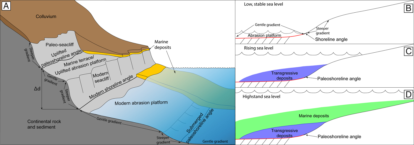
Figure 2. Morphology of onshore marine terraces and submerged abrasion platforms adapted from Haaker et al. (Reference Haaker, Rockwell, Kennedy, Ludwig, Freeman, Zumbro, Mueller and Edwards2016) and Klotsko et al. (Reference Klotsko, Driscoll, Kent and Brothers2015). (A) Diagram depicting the relationship between the wave-cut abrasion platform, paleosea cliff, paleoshoreline angle, and modern shoreline features. The Δd marks the difference in elevation between the modern shoreline and an uplifted paleoshoreline. This elevation difference is due to uplift, combined with potentially higher sea level during formation of the paleoshoreline. (B) A schematic depicting abrasion platforms that formed during sea-level low stands or slowdowns in the rate of sea-level rise, which are now submerged. Red line highlights the abrasion platform. Changes in the slope of the transgressive surface indicate paleoshoreline angles. (C) As sea level rises, sediment gets reworked and is deposited above the shoreline angle. These sediments are interpreted as transgressive deposits. (D) A high stand in sea level is marked by the maximum flooding surface (dark blue line) and the deposition of marine sediments. (For interpretation of the references to color in this figure legend, the reader is referred to the web version of this article.)
On uplifting coastlines, high-stand abrasion platforms, sea cliffs, shoreline angles, and related deposits become elevated above the modern shoreline and are known as marine terraces (Fig. 2A). These terraces are subjected to subaerial erosion and depositional processes that can obscure their original morphology. The uplifted abrasion platforms may be covered by a thin layer of coastal and marine sediments that are overlain by colluvium. With constant uplift, a series of marine terraces creates a step-like morphology (Kern and Rockwell, Reference Kern, Rockwell, Fletcher and Wehmiller1992; Haaker et al., Reference Haaker, Rockwell, Kennedy, Ludwig, Freeman, Zumbro, Mueller and Edwards2016). The elevation and ages of preserved paleoshoreline angles on these marine terraces are commonly used to reconstruct sea level, uplift, and deformation histories for the region (Kern and Rockwell, Reference Kern, Rockwell, Fletcher and Wehmiller1992; Kelsey and Bockheim, Reference Kelsey and Bockheim1994; Muhs et al., Reference Muhs, Simmons, Schumann, Groves, Mitrovica and Laurel2012; Muhs et al., Reference Muhs, Simmons, Schumann, Groves, Devogel, Minor and Laurel2014; Haaker et al., Reference Haaker, Rockwell, Kennedy, Ludwig, Freeman, Zumbro, Mueller and Edwards2016). Similar features can be formed during sea-level low stands and, on the same uplifting coastlines, may be preserved on the now-submerged continental shelf (Fig. 2A–D; Emery, Reference Emery1958; Darigo and Osborne, Reference Darigo, Osborne, Knight and McLean1986; Lajoie, Reference Lajoie and Wallace1986; Anderson, Reference Anderson, Densmore and Ellis1999; Chaytor et al., Reference Chaytor, Goldfinger, Meiner, Huftile, Romos and Legg2008; Klotsko et al., Reference Klotsko, Driscoll, Kent and Brothers2015). After formation, low stand paleoshoreline angles become submerged during subsequent sea-level rise, and may be buried by sediments deposited during sea-level rise and sea-level high stand. These deposits can conceal the paleoshoreline morphology at the seafloor (Fig. 2B–D).
High-stand paleoshorelines and associated marine terraces are preserved onshore the NCI, and provide a long-term record of tectonic vertical motion (Sorlien, Reference Sorlien, Halvorson and Maender1994; Dickinson, Reference Dickinson2001; Pinter et al., Reference Pinter, Sorlien and Scott2003; Muhs et al., Reference Muhs, Simmons, Schumann, Groves, Devogel, Minor and Laurel2014). Tectonic uplift rates can be estimated by determining the age and elevation of uplifted paleoshoreline angles and comparing these to a sea-level curve that provides the elevation of the paleoshoreline angle when it was created. Errors in determining uplift rates in this way can stem from uncertainties in measuring paleoshoreline angle elevations (i.e., GPS uncertainties, or presence of colluvium [Fig. 2]) and uncertainties in radiometric dating techniques. Furthermore, the choice of the sea-level curve used in the calculations can introduce errors. A eustatic sea-level curve can be used as an approximation, but eustatic sea-level curves do not reflect local to regional variability in Earth's response to loading of ice and water during ice sheet advance and retreat. In order to account for Earth's response to this loading, regional sea-level models can include an adjustment, known as the GIA. Regional sea-level curves that include GIA are spatially variable, even over short distances (Clark et al., Reference Clark, Mitrovica and Alder2004; Reeder-Myers et al., Reference Reeder-Myers, Erlandson, Muhs and Rick2015; Reynolds and Simms, Reference Reynolds and Simms2015; Simms et al., Reference Simms, Rouby and Lambeck2016). For example, the eustatic sea-level curve indicates the LGM sea level at 120 to 140 m below modern sea level (Lambeck et al., Reference Lambeck, Yokoyama and Purcell2002), while a GIA sea-level curve for the NCI reflects an LGM sea level of 106 m below modern sea level (Clark et al., Reference Clark, Mitrovica and Alder2014). There is variability in uplift rates calculated from marine terraces on the NCI, which may reflect variation in uplift rates between the locations of marine terraces used in each of the studies, or may be a result of uncertainty in the methods used, as stated above. Sorlien (Reference Sorlien, Halvorson and Maender1994) proposed uplift rates of 0.5–1.0 m/ka based on marine terraces from SRI and SCI, but these rates were based on inferred terrace ages, rather than direct radiometric dating. On SCI, the uranium-series dated 120 ka sea-level high-stand (MIS 5e) terrace is present, giving a maximum uplift rate of ~0.1 m/ka, with little to no uplift on the northwestern part of the island (Pinter et al., Reference Pinter, Lueddecke, Keller and Simmons1998; Pinter et al., Reference Pinter, Sorlien and Scott2003; Muhs et al., Reference Muhs, Simmons, Schumann, Groves, Devogel, Minor and Laurel2014). More recent work by Muhs et al. (Reference Muhs, Simmons, Schumann, Groves, Devogel, Minor and Laurel2014) dated the MIS 5a and MIS 5c/5e terraces on SRI and San Miguel Island using uranium-series dating and amino acid geochronology and determined an uplift rate of 0.12–0.20 m/ka. The lower uplift rates of Muhs et al. (Reference Muhs, Simmons, Schumann, Groves, Devogel, Minor and Laurel2014) were calculated with a GIA sea-level curve for San Nicolas Island (Fig. 1; Muhs et al., Reference Muhs, Simmons, Schumann, Groves, Mitrovica and Laurel2012; Muhs et al., Reference Muhs, Simmons, Schumann, Groves, Devogel, Minor and Laurel2014).
Submerged abrasion platforms have also been recognized around the NCI, and were first described by Emery (Reference Emery1958) based on single-beam bathymetric profiles. Emery (Reference Emery1958) identified five abrasion platforms between ~15–130 m below sea level (bsl) offshore the NCI. Later, Chaytor et al. (Reference Chaytor, Goldfinger, Meiner, Huftile, Romos and Legg2008) mapped submerged abrasion platforms and paleoshorelines around the NCI using high-resolution multibeam bathymetry. Chaytor et al. (Reference Chaytor, Goldfinger, Meiner, Huftile, Romos and Legg2008) also identified five paleoshorelines on the eastern NCI platform offshore SCI, with paleoshoreline depths ranging from ~22–90 m bsl. Chaytor et al. (Reference Chaytor, Goldfinger, Meiner, Huftile, Romos and Legg2008) interpreted an LGM paleoshoreline at ~90 m bsl and used the age, elevation, and eustatic sea-level curve of Lambeck et al. (Reference Lambeck, Yokoyama and Purcell2002) to generate an uplift rate of ~1.5 m/ka for the past ~23 ka. However, the Lambeck et al. (Reference Lambeck, Yokoyama and Purcell2002) sea-level curve did not account for local GIA and, therefore, the uplift rate may be overestimated because eustatic sea level at the LGM was lower than relative LGM sea level at the NCI (Clark et al., Reference Clark, Mitrovica and Alder2014; Muhs et al., Reference Muhs, Simmons, Schumann, Groves, Devogel, Minor and Laurel2014). Furthermore, both previous efforts to map submerged paleoshorelines around the NCI relied on modern seafloor data, but these data may conceal paleoshoreline morphology that has been buried by syn- and post-sea-level rise sedimentation (Fig. 2B–D). The lower uplift rate estimates for the islands are more consistent with regional uplift rates from southern California of 0.13–0.27 m/ka (Ku and Kern, Reference Ku and Kern1974; Kern and Rockwell, Reference Kern, Rockwell, Fletcher and Wehmiller1992; Grant et al., Reference Grant, Mueller, Gath, Cheng, Edwards, Munro and Kennedy1999; Mueller et al., Reference Mueller, Kier, Rockwell and Jones2009; Haaker et al., Reference Haaker, Rockwell, Kennedy, Ludwig, Freeman, Zumbro, Mueller and Edwards2016) than with uplift rates within the onshore Transverse Range province (Muhs et al., Reference Muhs, Simmons, Schumann, Groves, Devogel, Minor and Laurel2014; Rockwell et al., Reference Rockwell, Clark, Gamble, Oskin, Haaker and Kennedy2016). Recent measurements of vertical motion on SCI and SRI using GPS stations north of the SCIF and SRIF show a slight (< 0.5 mm/yr) subsidence (Hammond et al., Reference Hammond, Burgette, Johnson and Blewitt2018).
METHODS
In June 2016, ~190 km of high-resolution sub-bottom Chirp survey lines were acquired offshore of the NCI from the National Oceanic and Atmospheric Administration's (NOAA) R/V Shearwater using Scripps Institution of Oceanography's Edgetech 512i Chirp sub-bottom profiler. These data, collected as part of a study funded by the Bureau of Ocean Energy Management (BOEM), provide sub-bottom penetration up to ~50 m and sub-meter vertical resolution. Chirp line spacing was variable due to ship time constraints, but was ~300 m east of SCI, 360–620 m between SCI and SRI, and 450–700 m north of SRI (Fig. 1B). Some additional, longer lines with larger spacing were also collected as an exploratory survey. Chirp data were processed using SIOSEIS and Seismic Unix software to remove heave artifacts and adjust gains. Data were imported into IHS Kingdom Suite software package (http://www.kingdom.ihs.com) and ESRI ArcGIS v. 10.5 (http://www.esri.com) for interpretation. Kingdom Suite was used to calculate layer thicknesses and the depth to acoustic reflectors. A nominal sound velocity of 1500 m/s was used to convert time to depth.
Paleoshoreline angles were mapped in Chirp data by identifying the morphology illustrated in Figure 2. Gently sloping abrasion platforms that change to become steeper in slope were interpreted to represent a potential paleoshoreline angle. Once this morphology was identified, the paleoshoreline angle was picked as the point between the gentle and more steeply sloping sections of the profile (Fig. 2B–D). The depth of each paleoshoreline angle was determined by the two-way travel time recorded in the Chirp profile and corrected for Chirp towfish depth and tides. The following equation was used to calculate true depth:
 $$Depth_{True} = Depth_{TWTT} + Depth_{Chirp} + Tide$$
where Depth True is true depth, Depth TWTT is two-way travel time depth determined directly from Chirp profiles and using a nominal 1500 m/s sound velocity, Depth Chirp is depth of the Chirp towfish determined from pressure sensor readings stored in the trace headers, and Tide is a tide correction. The tide correction is the deviation from mean sea level that was acquired from the nearest NOAA station, 9411340, in Santa Barbara, CA (~67 km north of the NCI; http://www.tidesandcurrents.noaa.gov) at the specific date and time each Chirp line was collected. The average tidal range for the station is ~1.1 m.
It is important to consider the structural controls of the NCI and the lithology of bedrock when evaluating paleoshoreline angles in sub-bottom data. Faults and fluvial channels are common geologic influences in the NCI, whose features can have similar acoustic character to that of a paleoshoreline (i.e., change in slope of an erosive surface that resembles an abrasion platform), but are produced under conditions unrelated to sea-level change. To account for uncertainty related to faulting and paleochannels, each paleoshoreline angle was assigned a confidence level based on morphology and location relative to potential channels and fault zones. Interpretations were ranked as high confidence if they exhibited clear evidence of an abrasion platform and paleoshoreline angle. Additionally, these paleoshoreline angles were not interpreted near a fault zone or paleochannel, or could be identified as separate from fault zone deformation or channel morphology. Interpretations were ranked as medium confidence if they were either associated with a less distinct change in slope between the wave abrasion platform and paleoshoreline angle, or if it is possible that their morphology is influenced by a fault zone. Interpretations were ranked as low confidence if the survey line was near (<500 m) a fault zone or paleochannel and could not be clearly distinguished as separate from these features. Paleoshoreline angles picked as low confidence were not included in the binning strategy discussed below.
The true depth of paleoshoreline angles from individual Chirp profiles were binned based on apparent clustering of their depths and the location of each paleoshoreline angle. For example, if adjacent Chirp profiles had paleoshoreline angles that appeared to align roughly parallel to bathymetric contours and had a similar depth, these were included in the same bin. Once binned, the mean, standard deviation, and range of each bin were calculated, excluding the low confidence paleoshoreline angles (Table 1). The largest depth range for any of the bins was 11 m. We expect that a range of paleoshoreline true depths may reflect the same paleoshoreline due to uncertainty in picking the paleoshoreline angle and because relative sea-level rise and uplift rate can vary even across short distances, (Clark et al., Reference Clark, Mitrovica and Alder2014; Reeder-Myers et al., Reference Reeder-Myers, Erlandson, Muhs and Rick2015; Simms et al., Reference Simms, Rouby and Lambeck2016). Variability in paleoshoreline depth around the NCI was also observed in previous mapping of submerged abrasion platforms and paleoshorelines (Emery, Reference Emery1958; Chaytor et al., Reference Chaytor, Goldfinger, Meiner, Huftile, Romos and Legg2008), and onshore marine terraces are also mapped at variable elevation, possibly related to faulting (Pinter et al., Reference Pinter, Lueddecke, Keller and Simmons1998; Pinter et al., Reference Pinter, Sorlien and Scott2003; Muhs et al., Reference Muhs, Simmons, Schumann, Groves, Devogel, Minor and Laurel2014). Based on the geometry of paleoshoreline angles identified in adjacent Chirp profiles, we gain confidence that the paleoshoreline angles binned together reflect a single paleoshoreline, despite a range in depth. It cannot be ruled out, however, that the observed paleoshoreline angles may actually represent more, or fewer, true paleoshorelines than those interpreted here. Dating of sediments from the paleoshoreline angles, or more dense Chirp profile gridding, could help to resolve some of this uncertainty.
Table 1. Binned paleoshorelilne angle data

The mean depth and range for each bin was plotted at present time on a relative sea-level curve (age versus depth) to estimate the age of each paleoshoreline. A straight line was then drawn back in time, starting from the mean bin depth at present. This was completed for three different scenarios of uplift, where the slope of the plotted line is equal to the uplift rate. The effect of this is to plot the actual depth of the paleoshoreline if it had formed at various times in the past, essentially reversing the uplift. The three uplift rates chosen were 0 m/ka, representing no uplift, 0.16 m/ka, the average rate calculated by Muhs et al. (Reference Muhs, Simmons, Schumann, Groves, Devogel, Minor and Laurel2014), and 1.5 m/ka, the average rate calculated by Chaytor et al. (Reference Chaytor, Goldfinger, Meiner, Huftile, Romos and Legg2008). The relative sea-level curves used were derived by Clark et al. (Reference Clark, Mitrovica and Alder2014) for SRI (0–21 ka) and Muhs et al. (Reference Muhs, Simmons, Schumann, Groves, Mitrovica and Laurel2012) for San Nicolas Island (21–120 ka). Any point where the uplift rate model crosses the sea-level curve represents a possible time when that paleoshoreline formed (assuming constant uplift rates over the last ~120 ka). For each paleoshoreline, each point of intersection between the sea-level curve and uplift rate line provides a y-value representing the depth of formation and an x-value representing the time of formation. Abrasion platforms and associated shorelines form during periods of relatively stable sea level in which there is enough time for sea level to erode continental sediment via wave-base erosion. Therefore, if the uplift rate model intersects the sea-level curve during a period of slow change or stability in the independently derived sea-level curves, we interpreted this to be a likely candidate for formation of the paleoshoreline.
RESULTS
Regional angular unconformity
A regional angular unconformity was identified in Chirp profiles and mapped throughout the study area. The unconformity surface is characterized by a high-amplitude reflector and is identified by dipping and truncated reflectors below (Fig. 3–7). The unconformity is generally the highest amplitude reflector beneath the seafloor. However, the reflector varies in amplitude in portions of the study area between SRI and SCI. In areas where the unconformity was difficult to identify based on stratal geometry, it was traced laterally from regions where it could be confidently identified. In some areas north of SRI and east of SCI, the regional unconformity is also the seafloor. In other areas, the surface is overlain by two units of different acoustic character, with variable geometries including downlapping reflectors. Beneath the unconformity, folded and dipping reflectors are observed. The regional angular unconformity surface was mapped to identify topographic features and changes in slope. Within the mapped extent, the surface ranges between ~10–100 m bsl and shallows as it approaches the coastlines of SRI and SCI (Fig. 8). Several changes in slope of the regional unconformity were observed and interpreted as paleoshoreline angles, which are discussed in Paleoshorelines.

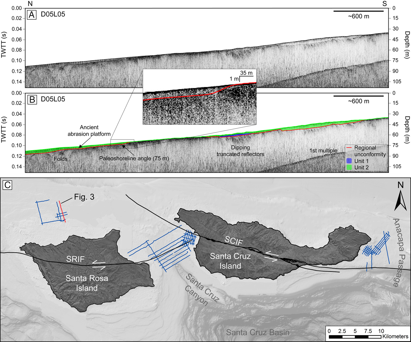
Figure 3. (color online) Chirp profile D05L05 north of SRI with (A) uninterpreted and (B) interpreted versions. Folded beds are observed to the north. (C) shows the profile location. Moving toward the south along the ancient abrasion platform, a 75-m paleoshoreline angle is observed at the base of the change in slope in the regional unconformity. The 75-m paleoshoreline angle is binned to the 83-m paleoshoreline. The regional unconformity is exposed at the seafloor in a portion of the survey. Unit 2 (~4 m thick) infills the 75-m paleoshoreline angle and thins landward. Changes in the slope of the regional unconformity to the south are not interpreted as paleoshoreline angles, as they are angled away from SRI's modern shoreline.

Figure 4. (color online) Northeast segment of Chirp profile D02L04b between SRI and SCI with (A) uninterpreted and (B) interpreted versions. (C) shows the profile location. The regional unconformity and unit boundaries are dashed where uncertain. Moving toward the northeast along the ancient abrasion platforms, 45- and 50-m paleoshoreline angles are observed at the base of the change in slope in the regional unconformity. The top reflector of Unit 1 terminates by onlapping onto the regional unconformity. Unit 2 thins landward. The 50-m paleoshoreline angle is binned to the 57-m paleoshoreline and is infilled by Unit 2 (~11 m thick). The 45-m paleoshoreline angle is binned to the 44-m paleoshoreline and is infilled by Unit 1 (~3 m thick) and Unit 2 (~3 m thick).
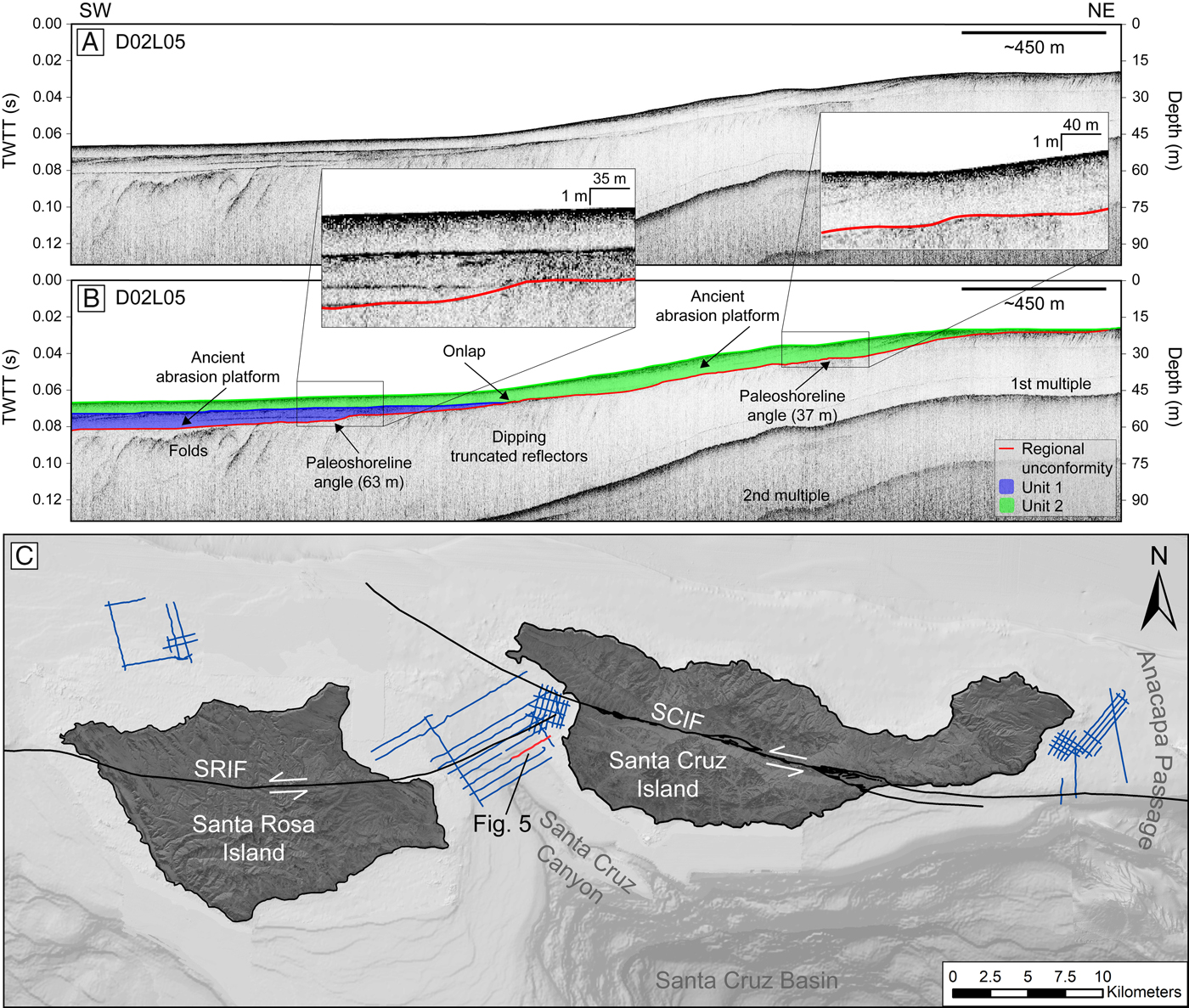
Figure 5. (color online) Northeast segment of Chirp profile D02L05 between SRI and SCI with (A) uninterpreted and (B) interpreted versions. (C) shows the profile location. Folded beds are observed to the southwest. The top reflector of Unit 1 terminates by onlapping onto the regional unconformity. Unit 1 and Unit 2 thin landward. Moving toward the northeast along the ancient abrasion platforms, 37- and 63-m paleoshoreline angles are observed at the base of the change in slope in the regional unconformity. The 37-m paleoshoreline angle is binned to the 36-m paleoshoreline and is infilled by Unit 2 (~7 m thick). The 63-m paleoshoreline angle is binned to the 66-m paleoshoreline and is infilled by Unit 1 (~6 m thick) and Unit 2 (~4 m thick).
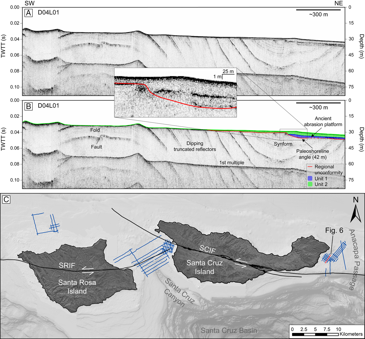
Figure 6. (color online) Chirp profile D04L01 east of SCI with uninterpreted (A) and interpreted (B) versions. (C) shows the profile location. The regional unconformity is dashed where uncertain. Here, the regional unconformity is exposed at the seafloor. Unit 1 and Unit 2 thin landward. A 42-m paleoshoreline angle is observed at the base of the change in slope in the regional unconformity. The 42-m paleoshoreline angle is binned to the 44-m paleoshoreline. Unit 1 (~3 m thick) and Unit 2 (~4 m thick) infill the 42-m paleoshoreline angle.

Figure 7. (color online) Chirp profile D04L15 east of SCI with (A) uninterpreted and (B) interpreted versions. (C) shows the profile location. Dipping and folded reflectors are observed below the regional unconformity, which is exposed at the seafloor to the southwest in the profile. Moving toward the southwest along the ancient abrasion platforms, 84- and 104-m paleoshoreline angles are observed at the base of the change in slope in the regional unconformity. The 84-m paleoshoreline angle is binned to the 83-m paleoshoreline, while the 104-m paleoshoreline angle is the only observed paleoshoreline angle at that depth. The 84-m paleoshoreline angle is infilled by Unit 2 (~3 m thick), and the 104-m paleoshoreline angle is infilled by Unit 1 (~3 m thick) and Unit 2 (~18 m thick).
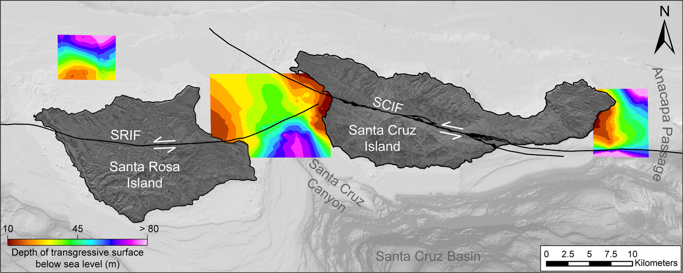
Figure 8. (color online) Interpolated surface of the regional unconformity interpreted to be the transgressive surface. The surface ranges between ~10–100 m below sea level and shallows as it approaches the coastlines of Santa Rosa Island (SRI) and Santa Cruz Island (SCI).
Acoustic units
Stratigraphy overlying the regional angular unconformity was interpreted as two separate acoustic units: Unit 1 and Unit 2 (Fig. 3–7). The contacts between each unit are characterized by moderate to high amplitude, continuous reflectors. The units vary in thickness and extent across the study area (Fig. 9).
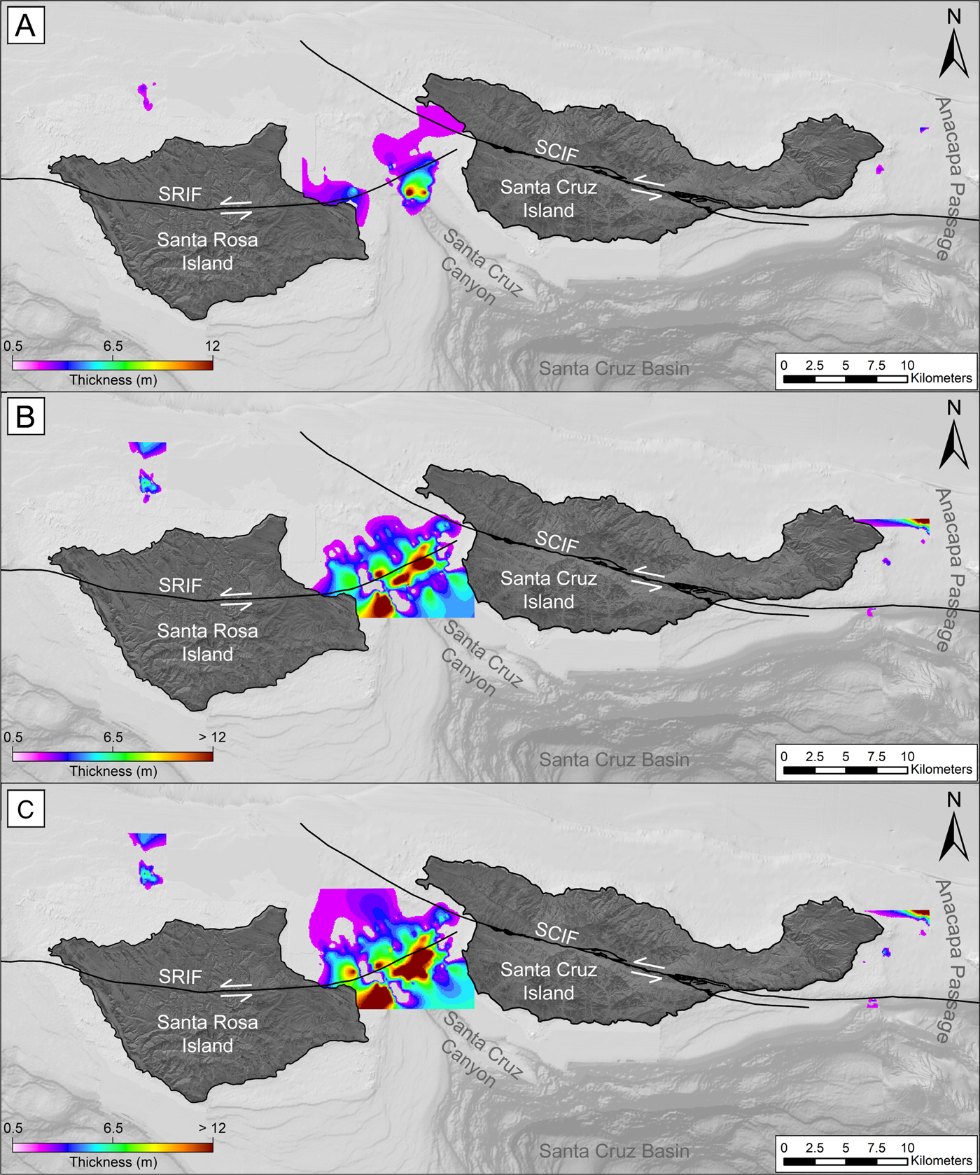
Figure 9. (color online) Isopach maps of sedimentary units. (A) Unit 1 isopach of transgressive deposits. Unit 1 thickness is greatest where there is an increase in slope in the underlying regional unconformity (Fig. 8). (B) Unit 2 isopach of marine Holocene deposits. Unit 2 thins landward and exhibits thickness variability both parallel and perpendicular to modern shorelines. (C) Isopach between the seafloor and transgressive surface. Zero thickness is displayed in areas where the transgressive surface becomes the seafloor. Variable thickness illustrates a difference in topography between the seafloor and sub-bottom surfaces.
Unit 1 is bounded at the bottom by the high-amplitude reflector identified as the regional angular unconformity and at the top by a reflector of moderate amplitude that diminishes intermittently throughout the study area. The upper reflector of Unit 1 terminates in some locations by onlapping onto the regional angular unconformity (e.g., Fig. 4 and 5). In other areas, the amplitude decreases and the reflector can no longer be traced laterally. Unit 1 is primarily observed between SRI and SCI, is mapped ~20–75 m bsl, and is not present in all portions of the study area. Where present, Unit 1 contains discontinuous, low-amplitude internal reflectors. Throughout the survey area, Unit 1 does not exceed 12 m in thickness (Fig. 9A). This maximum thickness, however, is only observed approaching the west side of Santa Cruz Canyon. Unit 1 does not exceed 8 m in thickness throughout the remainder of the survey area.
Unit 2 overlies Unit 1 or, in areas where Unit 1 is not present, the regional angular unconformity. Unit 2 thins landward and is not present where the regional angular unconformity is exposed at the seafloor north of SRI and east of SCI (Fig. 9B). Where Unit 1 is present, Unit 2 is bounded at the bottom by a reflector of moderate amplitude associated with the top of Unit 1 and at the top by the seafloor. Where Unit 1 is not present, Unit 2 is bounded at the bottom by the regional angular unconformity and at the top by the seafloor. Unit 2 is acoustically transparent and displays thickness variability both parallel and perpendicular to the inner shelf (Fig. 9B). It is observed between ~20–100 m bsl. Although mostly transparent, Unit 2 contains some high- and low-amplitude internal reflectors that are discontinuous. East of SCI where Unit 1 is not observed, Unit 2 fills in lows in the angular unconformity surface (Fig. 9A and B).
Paleoshorelines
Evidence of paleoshoreline angles was identified at 40 individual locations in Chirp profiles, with 31 locations identified as medium-high confidence (Fig. 10A, Table 1). Only the medium-high confidence paleoshoreline angles are considered in the subsequent discussion to limit the possibility of grouping faults or channel morphology with paleoshorelines. Paleoshoreline angles were defined on the regional angular unconformity surface by a change in slope from low-gradient (representing an abrasion platform) to a landward higher gradient (representing the paleo sea cliff; Fig. 2B-D). As defined in previous works, this intersection of abrasion platform and sea cliff represents the shoreline angle (Lajoie, Reference Lajoie and Wallace1986; Kern and Rockwell, Reference Kern, Rockwell, Fletcher and Wehmiller1992; Anderson et al., Reference Anderson, Densmore and Ellis1999; Grant et al., Reference Grant, Mueller, Gath, Cheng, Edwards, Munro and Kennedy1999; Chaytor et al., Reference Chaytor, Goldfinger, Meiner, Huftile, Romos and Legg2008; Muhs et al., Reference Muhs, Simmons, Schumann, Groves, Mitrovica and Laurel2012; Muhs et al., Reference Muhs, Simmons, Schumann, Groves, Devogel, Minor and Laurel2014; Haaker et al., Reference Haaker, Rockwell, Kennedy, Ludwig, Freeman, Zumbro, Mueller and Edwards2016). The true depths of the mapped paleoshoreline angles range from 27.6 to 104.0 m bsl, which were binned into seven paleoshorelines (Table 1). Paleoshoreline interpretations connect paleoshoreline angles in different Chirp profiles and then are inferred to extend roughly parallel to the modern shoreline and bathymetric contours (Fig. 10).
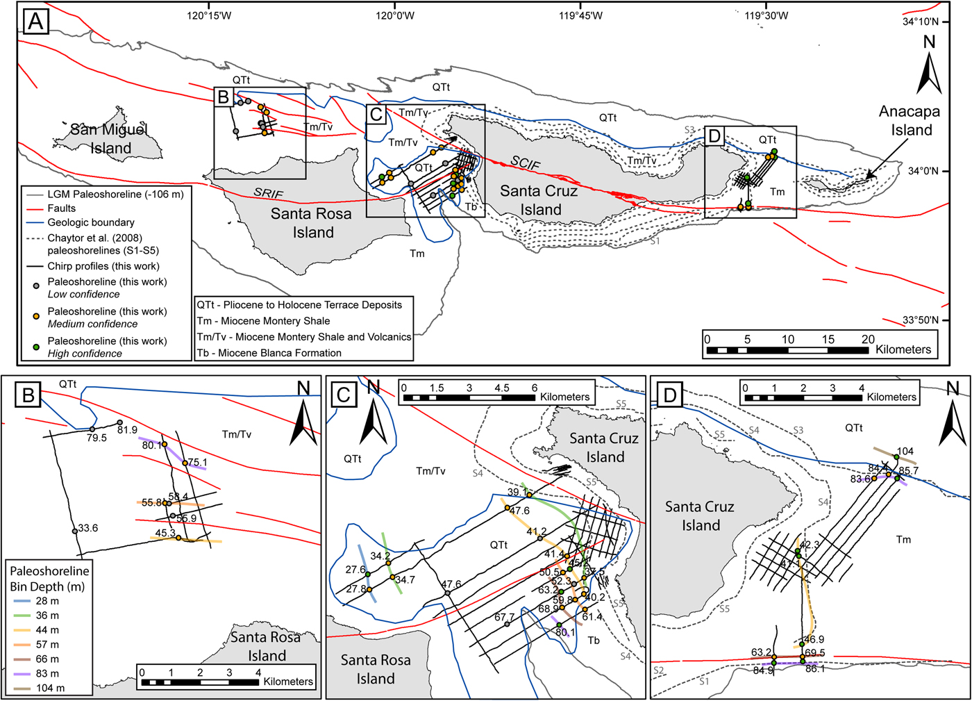
Figure 10. (color online) (A) Map of the Northern Channel Islands, showing paleoshoreline angle locations on Chirp survey lines, with various other relevant geomorphic and geologic features, including: faults; the geologic boundary between Quaternary terrace deposits (QTt) and older formations (Tm, Tv, Tb); Chaytor et al. (Reference Chaytor, Goldfinger, Meiner, Huftile, Romos and Legg2008) mapped paleoshorelines, labeled by name (S1–S5); the -106-m-depth contour, which would reflect the LGM paleoshoreline based on the sea-level curve of Clark et al. (Reference Clark, Mitrovica and Alder2014) and modern bathymetric data. See legend for additional details. SRIF, Santa Rosa Island Fault; SCIF, Santa Cruz Island Fault. Black boxes mark locations of zoomed in maps shown in (B–D). (B– D) include the same content as (A), but with the addition of the mapped interpreted paleoshorelines, which are all colored by the legend shown in (B).
The 28-m paleoshoreline is observed in two Chirp profiles between SRI and SCI (Table 1, Fig. 10). The paleoshoreline angles are sharp and infilled by Unit 1 and Unit 2. The abrasion platforms and paleoshoreline angles in each location exhibit the characteristic morphology of uplifting coastlines, with a more gently sloping abrasion platform and a landward, more steeply dipping paleoshoreline angle. Neither the SRIF nor the SCIF are in proximity to the 28-m paleoshoreline (Fig. 10).
The 36-m paleoshoreline is observed in four Chirp profiles between SRI and SCI (Table 1, Fig. 10). Characteristic abrasion platform-paleoshoreline angle morphology is observed in all locations with gradual changes in the slope of the regional angular unconformity between the abrasion platform and paleoshoreline angle (Fig. 5). Each paleoshoreline angle is infilled by Unit 2.
The 44-m paleoshoreline is observed north of SRI in one Chirp profile, between SRI and SCI in four Chirp profiles, and east of SCI in three Chirp profiles (Table 1, Fig. 10). In areas north of SRI and between SRI and SCI, the paleoshoreline angle is observed as a gentle increase in the slope of the regional angular unconformity, while in locations between SRI and SCI that are <500 m from the SRIF, and all locations east of SCI, paleoshoreline angles appear steeper (Fig. 4 and 6). The paleoshoreline north of SRI is infilled by Unit 2. Between SRI and SCI, paleoshorelines are infilled by Unit 1 and Unit 2, or only by Unit 2 (Fig. 4). In locations east of SCI, paleoshorelines are infilled by Unit 1 and Unit 2 (Fig. 6), or are not overlain by any sediment.
The 57-m paleoshoreline is observed in one Chirp profile north of SRI and three profiles between SRI and SCI (Table 1, Fig. 10). The regional angular unconformity in each location exhibits a gradual change in slope and is infilled by Unit 2 (Fig. 4). Neither the SRIF nor the SCIF are in the proximity of the 57-m paleoshoreline. Abrasion platform and paleoshoreline morphology is similar between the four locations.
The 66-m paleoshoreline is observed in two Chirp profiles between SRI and SCI and two profiles east of SCI (Table 1, Fig. 10). Between SRI and SCI, the regional unconformity exhibits a gradual change in slope and is infilled by Unit 1 and Unit 2 (Fig. 5). East of SCI, the regional unconformity appears to exhibit a sharp change in slope at the paleoshoreline angle and is infilled by Unit 2. The morphology of the abrasion platform and paleoshoreline angle amongst the 66-m paleoshoreline is similar.
The 83-m paleoshoreline is observed in two Chirp profiles north of SRI, in one profile between SRI and SCI, and in five profiles east of SCI (Table 1, Fig. 10). Each location exhibits similar morphology and the paleoshoreline angle is marked by a gradual change in the slope of the regional unconformity (Fig. 3 and 7). Additionally, Unit 2 infills the slope at each location except for the two paleoshoreline angles southwest of SCI.
The 104-m paleoshoreline is observed in one Chirp profile east of SCI (Fig. 10). The paleoshoreline angle exhibits a gradual change in slope (Fig. 7). It is noted that the profile makes a turn just seaward of the interpreted paleoshoreline angle. The lower abrasion platform in this area therefore may not be as flat as it appears in the profile. The paleoshoreline angle is infilled by both Unit 1 and Unit 2. Additionally, neither the SRIF nor the SCIF are in the proximity of paleoshoreline locations.
DISCUSSION
Transgressive surface
The regional angular unconformity observed throughout the study area is interpreted to be the transgressive surface that formed as sea level rose following the LGM (Posamentier and Allen, Reference Posamentier and Allen1993; Hogarth et al., Reference Hogarth, Driscoll, Babcock and Orange2012). However, this part of the shelf has been subaerially exposed during many sea-level low stands in the Pleistocene and the current morphology probably reflects multiple sea-level cycles, as opposed to strictly the most recent sea-level rise (Hogarth et al., Reference Hogarth, Babcock, Driscoll, Le Dantec, Haas, Inman and Masters2007).
Sediment units
Based on geometry and acoustic character, Unit 1 is interpreted to be transgressive deposits, which form during periods of rising relative sea level, when accommodation outpaces sediment supply (Posamentier, Reference Posamentier2002; Lantzsch et al., Reference Lantzsch, Hanebuth, Bender and Krastel2009; Schwab et al., Reference Schwab, Baldwin, Denny, Hapke, Gayes, List and Warner2014; Klotsko et al., Reference Klotsko, Driscoll, Kent and Brothers2015). The location of this unit, often observed at, and onlapping onto, paleoshoreline angles, along with the presence of internal, low-amplitude reflectors, is consistent with transgressive deposits described elsewhere on the southern California continental shelf (Hogarth et al., Reference Hogarth, Babcock, Driscoll, Le Dantec, Haas, Inman and Masters2007; Le Dantec et al., Reference Le Dantec, Hogarth, Driscoll, Babcock, Barnhardt and Schwab2010; Klotsko et al., Reference Klotsko, Driscoll, Kent and Brothers2015). Additionally, transgressive deposits are relatively thin due to the rapid landward migration that transgressive shorelines make in areas of low elevation (Cattaneo and Steel, Reference Cattaneo and Steel2003), which is consistent with the isopach of Unit 1 (Fig. 9A).
Unit 2 is interpreted to be marine Holocene sediment deposited during sea-level high stand. Marine high-stand sediments deposit over transgressive deposits, or the transgressive surface, once the shoreline has transgressed landward (Posamentier and Allen, Reference Posamentier and Allen1999). During the most recent sea-level transgression, the rate of sea-level rise decreased when the shoreline was ~10 m below present at ~7 ka (Clark et al., Reference Clark, Mitrovica and Alder2014). Therefore, deposition of Unit 2 likely began around this time. The average thickness of this unit is within the range of other mapped Holocene marine sediment units on the southern California continental shelf (Hogarth et al., Reference Hogarth, Babcock, Driscoll, Le Dantec, Haas, Inman and Masters2007; Le Dantec et al., Reference Le Dantec, Hogarth, Driscoll, Babcock, Barnhardt and Schwab2010; Klotsko et al., Reference Klotsko, Driscoll, Kent and Brothers2015).
Submerged paleoshoreline mapping
It is important to consider the structural controls of the NCI when evaluating paleoshoreline angles in sub-bottom data. Faults and fluvial channels are common geologic influences in the NCI, whose features can have similar acoustic character to that of a paleoshoreline (i.e., change in slope of the transgressive surface), but are produced under conditions unrelated to sea-level change. The SRIF trends east-west through SRI, while the SCIF trends northwest-southeast through SCI. Both faults demonstrate predominantly left-lateral, strike-slip motion, with some vertical component of slip (Patterson, Reference Patterson1979; Pinter et al., Reference Pinter, Lueddecke, Keller and Simmons1998; Pinter and Sorlien, Reference Pinter and Sorlien1991). These faults could produce scarps that have no relation to shorelines that formed during sea-level low stands. Additionally, small bends in these faults could produce localized areas of transpression and uplift that may impact paleoshoreline depths. There is also evidence in Chirp data of ancient fluvial channels offshore the NCI that formed during the LGM by incision and downcutting. The banks of these channels exhibit a similar morphology to that of a paleoshoreline, but are independent of the development of the NCI's paleoshorelines. The confidence ranking for each individual paleoshoreline angle described in Methods was used to minimize interpretation of faults and fluvial channels as paleoshorelines. Despite this ranking, there are two locations where interpreted paleoshorelines could actually represent fault scarps (Fig. 10). The 44-, 57-, and 83-m paleoshorelines north of SRI all trend roughly parallel to unnamed discontinuous faults, although not directly on top of them (Fig. 10A). However, direct evidence of offset beds beneath the mapped paleoshoreline angles was not observed in any of the Chirp profiles. The 66-m paleoshoreline mapped east of SCI is also parallel and very close to the mapped SCIF (Fig. 10D). Since the fault and paleoshoreline are mapped across a steep slope with poor imaging in the Chirp profiles, it is difficult to identify evidence of any structures below the regional unconformity in this location, so a fault scarp cannot be ruled out. Nevertheless, in all four of these cases, there are paleoshorelines mapped elsewhere at similar depths that are not adjacent to faults. Therefore, we maintain the interpretation of these features as paleoshorelines.
The lithology of bedrock is also an important consideration for interpretation of paleoshorelines, as softer sedimentary beds will erode more easily than harder or more lithified rocks and result in relatively larger wave-cut platforms for the same amount of wave exposure and energy. This, however, likely only had a minimal impact on paleoshoreline angles and associated paleoshorelines that were interpreted, as most of the underlying bedrock on the continental shelf is mapped as Miocene sedimentary units that are expected to exhibit similar erosional patterns (Junger, Reference Junger1979). There is a mapped geologic contact between Miocene Monterey shale formation (Tm) and Quaternary terrace deposits (QTt) along the north side of the NCI platform that runs roughly parallel to bathymetric contours and adjacent to the 83-m and 104-m paleoshorelines east of SCI (Fig. 10). In legacy seismic data from the 1979 Junger report, adjacent to this location, the QTt deposits are imaged as a wedge-shaped unit on the northern shelf edge and slope of the NCI platform, resting unconformably on the Tm formation that outcrops on the NCI platform between SCI and Anacapa Island. The contact appears to be imaged in the Chirp profile that captures the 104-m paleoshoreline angle (Fig. 7). In the Chirp profile, folded and dipping beds below the regional unconformity are interpreted as the Tm formation, while the mostly transparent Unit 2 is interpreted as QTt. This profile illustrates that the observed paleoshoreline angle morphology is different from the contact between the geologic units.
Two previous efforts to map the paleoshorelines surrounding the NCI using bathymetric data both resulted in identification of five submerged abrasion platforms and paleoshorelines (Table 2; Emery, Reference Emery1958; Chaytor et al., Reference Chaytor, Goldfinger, Meiner, Huftile, Romos and Legg2008). The depth of the Chaytor et al. (Reference Chaytor, Goldfinger, Meiner, Huftile, Romos and Legg2008) paleoshorelines does not always follow bathymetric depth contours, and there appears to be a noticeable difference in paleoshoreline depth between the shelf north of and south of SCI. North of SCI, four paleoshorelines are mapped at ~20 (S5), 48 (S4), and 80 (S3) m bsl. South of the island, the LGM paleoshoreline (S1) is mapped at ~90 m bsl and other paleoshorelines are mapped at ~15 (S5), 64 (S3), and 80 (S2) m bsl. Due to the depth variability of our paleoshorelines and the Chaytor et al. (Reference Chaytor, Goldfinger, Meiner, Huftile, Romos and Legg2008) paleoshorelines, and the reporting of only the deeper edge of the abrasion platform from Emery (Reference Emery1958), it is difficult to compare the paleoshorelines of each effort based only on depth (Table 2). In map view, however, it does appear that some of the paleoshorelines mapped here align with those of Chaytor et al. (2008; Fig. 10B–D).
Table 2. Table reporting the approximate paleoshoreline depths from previous work compared to the depths of paleoshorelines observed in sub-bottom data here. Both Chaytor et al. (Reference Chaytor, Goldfinger, Meiner, Huftile, Romos and Legg2008) and Emery (Reference Emery1958) used bathymetric data to map paleoshorelines.

a Chaytor et al. (Reference Chaytor, Goldfinger, Meiner, Huftile, Romos and Legg2008) depths estimated from their Figure 5, north-south profile across Santa Cruz Island. The authors did note that depths of their mapped shorelines were variable.
b Emery (Reference Emery1958) depths are reported as an average for offshore islands in the California Borderlands, including some islands south of the NCI. These are also measured at the seaward, deeper edge of the terrace, not the paleoshoreline angle.
c Reported as the LGM terrace.
d Reported as the shelf edge.
West of SCI, the 44-m paleoshoreline mapped in sub-bottom data is close to the S4 paleoshoreline of Chaytor et al. (2008; Fig. 10D), but on the west side of SCI the S4 paleoshoreline maps closer to our 36-m paleoshoreline (Fig. 10C). This could be a result of the binning strategy used here, or the fact that the Chaytor et al. (Reference Chaytor, Goldfinger, Meiner, Huftile, Romos and Legg2008) S4 paleoshoreline was mapped using bathymetric data, while the 36- and 44-m paleoshorelines were mapped here using sub-bottom data.
In the sub-bottom data northeast of SCI, we observed two paleoshorelines at ~80 and ~104 m bsl. The 104-m paleoshoreline does not correspond to any paleoshoreline mapped by Chaytor et al. (Reference Chaytor, Goldfinger, Meiner, Huftile, Romos and Legg2008) and is located ~2.5 km shoreward of the interpreted shelf edge at 100-m water depth (Fig. 10). In sub-bottom data, the 104-m paleoshoreline is blanketed by ~20 m of sediment that is interpreted as transgressive and Holocene marine sediment (Fig. 7). If this interpretation is correct, the 104-m paleoshoreline may represent the LGM paleoshoreline on the northern platform, which has implications for paleoshoreline and paleoenvironmental modeling that use modern bathymetric data, as the full LGM extent of the NCI platform would be smaller than predicted by modern bathymetry. Alternatively, the Unit 1 and Unit 2 deposits mapped in this area could be older, reworked sediment with the regional unconformity representing an older sea-level cycle. The 104-m paleoshoreline is not observed elsewhere in the sub-bottom data, but this may be due to lack of data coverage at that water depth.
South of Anacapa Passage, the slope is much steeper, and thin to no sediment is observed above the transgressive surface. Although binned with the 83-m paleoshoreline, the true depth of the 83-m paleoshorelines south of Anacapa Passage are ~85–86 m bsl (Fig. 10D). In this area, the 83-m paleoshoreline is geographically close to the LGM paleoshoreline (~90 m bsl) interpreted by Chaytor et al. (2008; Fig. 10D), and the discrepancy in depth may be related to the different types of data used, or the exact location that was picked to represent the paleoshoreline angle. North of Anacapa Passage, the 83-m paleoshoreline depths mapped in Chirp data are similar to those south of the Passage, but the northern 83-m paleoshoreline maps more closely to paleoshoreline S3 of Chaytor et al. (Reference Chaytor, Goldfinger, Meiner, Huftile, Romos and Legg2008). This discrepancy may be related to the thick sediment deposit observed above the 83 m paleoshoreline north of Anacapa Passage (Fig. 7), as the Chaytor et al. (Reference Chaytor, Goldfinger, Meiner, Huftile, Romos and Legg2008) paleoshorelines are based on bathymetric data. In other locations, our data do not intersect with mapped paleoshorelines from Chaytor et al. (Reference Chaytor, Goldfinger, Meiner, Huftile, Romos and Legg2008), so a correlation cannot be determined.
Uplift rate models and paleoshoreline ages
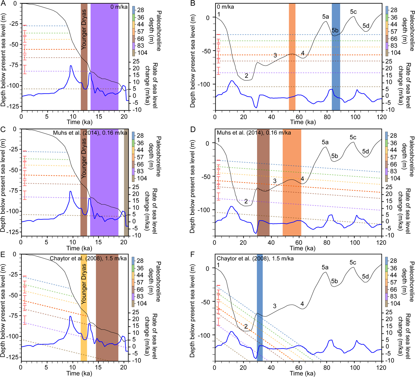
The paleoshoreline depths were compared to the Clark et al. (Reference Clark, Mitrovica and Alder2014) relative sea-level curve from 0–21 ka and the Muhs et al. (Reference Muhs, Simmons, Schumann, Groves, Mitrovica and Laurel2012) relative sea-level curve from 21–120 ka, for three uplift rate scenarios: (1) a stable NCI platform (0 m/ka uplift rate); (2) the average uplift rate (0.16 m/ka) determined by Muhs et al. (Reference Muhs, Simmons, Schumann, Groves, Devogel, Minor and Laurel2014); and (3) the average uplift rate (1.5 m/ka) determined by Chaytor et al. (2008; Fig. 11). We interpret any point where the modeled shoreline intersects the sea-level curve during a period of slow change or stability in sea level as a likely candidate for formation of the paleoshoreline.

Figure 11. Uplift rate models for the NCI used to reconcile the rate of late Quaternary uplift. The black curve represents the Clark et al. (Reference Clark, Mitrovica and Alder2014) relative sea-level curve from 0–21 ka (A, C, and E) and the Muhs et al. (Reference Muhs, Simmons, Schumann, Groves, Mitrovica and Laurel2012) relative sea-level curve from 21–120 ka (B, D, and F). Numbered labels represent marine isotope stages. The blue curve represents the rate of sea-level change over time calculated from the respective sea-level curves. At time zero, along the left hand y-axis, red vertical bars represent the depth range corresponding to each paleoshoreline bin, with the mean for that bin projected back in time using a dashed line of the color indicated in the key. The dashed line, representing the mean paleoshoreline depth, is projected onto the relative sea-level curves using various uplift rates that are reflected in the slope of the line. (A and B) A stable NCI platform (uplift rate 0 m/ka). (C and D) Muhs et al. (Reference Muhs, Simmons, Schumann, Groves, Devogel, Minor and Laurel2014) average uplift rate (0.16 m/ka). (E and F) Chaytor et al. (Reference Chaytor, Goldfinger, Meiner, Huftile, Romos and Legg2008) average uplift rate (1.5 m/ka). (For interpretation of the references to color in this figure legend, the reader is referred to the web version of this article.)
Modeled 0 m/ka uplift rate
Assuming a stable NCI platform (i.e., 0 m/ka uplift rate; Fig. 11A and B), the 28-, 36-, and 44-m paleoshorelines intersect the sea-level curve during a period of rapid sea-level rise (~15–16 mm/yr) following the LGM. They also all cross the curve during the sea-level fall (~4 mm/yr) between MIS 5a and MIS 4. During these times, it is unlikely that paleoshoreline angles would have formed due to the rapid rates of sea-level fluctuation. The 28-m paleoshoreline also intersects the sea-level curve during the MIS 5b low stand, which may have generated a paleoshoreline angle. It is also possible that these shallowest paleoshorelines were created during earlier sea-level cycles, as they would cross the sea-level curve again prior to 120 ka (Spratt and Lisiecki, Reference Spratt and Lisiecki2016).
The 57-m paleoshoreline intersects the sea-level curve during the minor high stand of MIS 3 at ~55 ka, which may have formed a paleoshoreline angle due to the stable sea level. The 66-m paleoshoreline crosses the sea-level curve at ~11.5 ka, near to the end of the Younger Dryas stade. The Younger Dryas stade represents a relatively slow rate of sea-level rise (~6.5 mm/yr) between more rapid periods of rise after the LGM, when a paleoshoreline angle could have formed. The 66-m paleoshoreline also intersects the sea-level curve at ~43 ka during sea-level fall in MIS 3. The slow sea-level fall here could potentially result in paleoshoreline angle formation, but we have lower confidence in this interpretation. The 83-m paleoshoreline intersects the curve during rapid sea-level rise prior to the Younger Dryas stade and again during rapid sea-level fall between MIS 3 and MIS 2. Due to the accelerated rate of sea-level change, these are both unlikely to have generated a paleoshoreline angle. However, the range of depths associated with this paleoshoreline could place the formation period during the time of slowly rising sea-level between ~18.5–13.5 ka. Finally, the 104-m paleoshoreline intersects the sea-level curve during a period of rapid sea-level rise after the LGM, which we interpret to be unlikely to form a paleoshoreline angle.
Modeled 0.16 m/ka uplift rate
Using the Muhs et al. (Reference Muhs, Simmons, Schumann, Groves, Devogel, Minor and Laurel2014) model (i.e., 0.16 m/ka uplift rate; Fig. 11C and D), the 28-, 36-, and 44-m paleoshorelines intersect the sea-level curve during a period of rapid sea-level rise (~15–16 mm/yr) following the LGM. They also all cross the curve during the sea-level fall (~4 mm/yr) between MIS 5a and MIS 4. There does not appear to be a time during the last 120 ka where sea level was stable enough to have created these paleoshoreline angles. However, it is possible that they were created during earlier sea-level cycles (Spratt and Lisiecki, Reference Spratt and Lisiecki2016).
The 57-m paleoshoreline intersects the sea-level curve at 10.8 ka and 45 ka. Of these, 10.8 ka is during a period of sea-level rise (~8 mm/yr) and 45 ka is during a period of slow sea-level fall (~1.5 mm/yr) during MIS 3, following the ~55 ka MIS 3 minor high stand. Muhs et al. (Reference Muhs, Simmons, Schumann, Groves, Devogel, Minor and Laurel2014) predicted the depth of this MIS 3 high-stand paleoshoreline to be ~55 m bsl based on their uplift rate for SRI. Klotsko et al. (Reference Klotsko, Driscoll, Kent and Brothers2015) observed an abrasion platform offshore San Onofre, California, at 72–53 m bsl in sub-bottom data that was attributed to the period of slower sea-level rise during the Younger Dryas stade, ~13–11.5 ka, using a eustatic sea-level curve. Although the 57-m paleoshoreline offshore the NCI occurs at a similar depth, it is difficult to assess whether these represent the same period of paleoshoreline formation as relative sea-level histories can vary over even short distances (Clark et al., Reference Clark, Mitrovica and Alder2014; Reeder-Myers et al., Reference Reeder-Myers, Erlandson, Muhs and Rick2015; Simms et al., Reference Simms, Rouby and Lambeck2016). Using the SRI relative sea-level curve (Clark et al., Reference Clark, Mitrovica and Alder2014), the paleoshoreline angle associated with the Younger Dryas stade is expected to be deeper than 57 m and outside the range of depths associated with this paleoshoreline. Therefore, we interpret the 57-m paleoshoreline to more likely have formed during MIS 3. The total range of depths for this paleoshoreline mostly fall during the sea-level fall after the 55 ka minor high stand, but the range also encompasses MIS 4.
The 66-m paleoshoreline intersects the sea-level curve at 11.9 ka, and three times between 29 and 39 ka. At 11.9 ka the rate of sea-level rise begins to increase following a slower sea-level rise (~6.5 mm/yr) from ~13–11.5 ka during the Younger Dryas stade. The other three times where the paleoshoreline crosses the relative sea-level curve are all near the second minor high stand of MIS 3 in the Muhs et al. (Reference Muhs, Simmons, Schumann, Groves, Mitrovica and Laurel2012) relative sea-level curve. It is therefore possible that the 66-m paleoshoreline and abrasion platform formed during MIS 3, ~29–39 ka, and were then reoccupied during the Younger Dryas stade.
The 83-m paleoshoreline intersects the sea-level curve at 13.8 ka and 27 ka. The former (13.8 ka) marks the initiation of rapid sea-level rise (~35 mm/yr) following a ~5 ka period of slower sea-level rise (18.5–13.5 ka). Where imaged, the seaward end of the abrasion platform associated with the 83-m paleoshoreline is ~92 m, which is close to the sea level at the start of the 18.5–13.5 ka decreased rate of sea-level rise, and appears to be a good candidate for paleoshoreline angle formation. The second crossing at 27 ka is during a period of rapid sea-level fall (~12 mm/yr) and likely does not correspond to paleoshoreline angle formation. The 104-m paleoshoreline intersects the Clark et al. (Reference Clark, Mitrovica and Alder2014) sea-level curve at 20 ka (LGM), and no other locations, and therefore may represent the LGM paleoshoreline.
Modeled 1.5 m/ka uplift rate
Using the Chaytor et al. (Reference Chaytor, Goldfinger, Meiner, Huftile, Romos and Legg2008) model (i.e., 1.5 m/ka uplift rate; Fig. 11E and F), the 28-m paleoshoreline intersects the sea-level curve at 9.6 ka and 29 ka. The intersection at 9.6 ka is within a period of rapid sea-level rise (~17.5 mm/yr) and unlikely to form a paleoshoreline angle, but 29 ka follows the second minor high stand of MIS 3, which is more likely to have formed a paleoshoreline angle. The 36-m paleoshoreline intersects the sea-level curve during periods of rapid sea-level rise (~14 mm/yr) and rapid sea-level fall (~18 mm/yr), neither of which are likely to have produced a paleoshoreline angle. The 44-m paleoshoreline intersects the sea-level curve at 11.1 ka and 27 ka. The intersection at 11.1 ka occurs near the end of the Younger Dryas stade with slower sea-level rise (~14 mm/yr) and 27 ka occurs during a period of rapid sea-level fall (~18 mm/yr). The 44-m paleoshoreline could be associated with the Younger Dryas stade. The mean depth appears to intersect the curve ~400 yr after the rapid post-Younger Dryas stade sea-level rise began, but the range of depths for this paleoshoreline include the initiation of rapid sea-level rise at ~11.5 ka. The 57-m paleoshoreline intersects the sea-level curve at 13 ka and 26 ka, periods of rapid sea-level rise (~20 mm/yr) and rapid sea-level fall, respectively. Both periods are unlikely to have produced an abrasion platform. The 66-m paleoshoreline occurs at 14.5 ka, during a period of slower sea-level rise from 18.5–13.5 ka, and appears to be a good candidate for paleoshoreline angle formation. Neither the 83-m nor 104-m paleoshorelines intersect the sea-level curves. Additionally, using the 1.5 m/ka uplift rate, none of the paleoshorelines would have been formed during previous sea-level cycles, as sea level has only fluctuated ~130 m over the past ~800 ka (Spratt and Lisiecki, Reference Spratt and Lisiecki2016).
Uplift rate model assessment
These results suggest that the Muhs et al. (Reference Muhs, Simmons, Schumann, Groves, Devogel, Minor and Laurel2014) uplift rate is a better fit to our submerged paleoshoreline data compared to the stable NCI platform scenario or the faster uplift rate of Chaytor et al. (Reference Chaytor, Goldfinger, Meiner, Huftile, Romos and Legg2008). Our preferred model is the Muhs et al. (Reference Muhs, Simmons, Schumann, Groves, Devogel, Minor and Laurel2014) uplift rate because this is the only scenario where the four deepest paleoshorelines appear to coincide with times of relatively stable or slowly rising sea level. In the Chaytor et al. (Reference Chaytor, Goldfinger, Meiner, Huftile, Romos and Legg2008) model, the two deepest terraces do not intersect the sea-level curves at all, which means these could not have been created by the processes that create abrasion platforms and paleoshoreline angles (i.e., wave-base erosion). Furthermore, if the Muhs et al. (Reference Muhs, Simmons, Schumann, Groves, Devogel, Minor and Laurel2014) uplift model is extended beyond 120 ka, the three shallowest paleoshorelines that do not appear to fit with the model could be explained by previous sea-level cycles; but using the Chaytor et al. (Reference Chaytor, Goldfinger, Meiner, Huftile, Romos and Legg2008) uplift rate, the shallowest paleoshorelines could not have been formed in previous sea-level cycles. The stable NCI platform model could also explain the shallowest paleoshorelines as formed during earlier intervals of the sea-level cycle. However, the deepest paleoshoreline does not correspond as closely to the LGM stable sea-level period as the Muhs et al. (Reference Muhs, Simmons, Schumann, Groves, Devogel, Minor and Laurel2014) model. The better fit of both low uplift rate models (0 and 0.16 m/ka) seems to at least indicate that an uplift rate on the lower end of previous estimates is a better fit to the submerged paleoshorelines mapped in sub-bottom data. Using the preferred uplift rate model, the interpreted ages of each paleoshoreline are presented in Table 1.
The uplift rate of ~0.16 m/ka is more consistent with uplift rates reported for the southern California region of 0.13–0.27 m/ka (Ku and Kern, Reference Ku and Kern1974; Kern and Rockwell, Reference Kern, Rockwell, Fletcher and Wehmiller1992; Grant et al., Reference Grant, Mueller, Gath, Cheng, Edwards, Munro and Kennedy1999; Mueller et al., Reference Mueller, Kier, Rockwell and Jones2009; Haaker et al., Reference Haaker, Rockwell, Kennedy, Ludwig, Freeman, Zumbro, Mueller and Edwards2016) than with uplift rates reported in the onshore Transverse Range province (Muhs et al., Reference Muhs, Simmons, Schumann, Groves, Devogel, Minor and Laurel2014; Rockwell et al., Reference Rockwell, Clark, Gamble, Oskin, Haaker and Kennedy2016). This suggests that the NCI platform is controlled by the regional forces responsible for uplift in southern California, rather than those uplifting the Transverse Ranges at higher rates. If uplift related to the Transverse Range province was initiated to the north and is southward stepping, the NCI, located at the southern extent of this province, may not yet have experienced significant uplift related to the transpression in the Transverse Ranges.
Assessment of uplift rates by this method has limitations. For example, the assumption of a constant uplift rate could result in mis-interpretation of paleoshoreline ages if uplift rates varied through time. Additionally, these results show that abrasion platforms and paleoshoreline angles could have been influenced by wave-base erosion at several time periods during the last ~120 ka and even during previous sea-level cycles, resulting in overprinting of morphology. This could result in more pronounced morphology on paleoshoreline angles that are reoccupied. On the other hand, paleoshorelines that are subjected to repeated erosional and reworking processes could be more difficult to define in the sub-bottom data. Finally, there are several sources of uncertainty in both estimates of paleoshoreline depths and the application of relative sea-level curves. Each modeled paleoshoreline depth represented a bin of observed paleoshoreline angle depths. Furthermore, uplift rate estimates from Muhs et al. (Reference Muhs, Simmons, Schumann, Groves, Devogel, Minor and Laurel2014) and Chaytor et al. (Reference Chaytor, Goldfinger, Meiner, Huftile, Romos and Legg2008) are reported as a range, but our model used the average rate of that range. Both of these uncertainties mean that the timing of paleoshoreline depth intersection with the sea-level curve is more of a range than an exact point reported by the model results. The best way to improve the uplift rate assessment would be to obtain radiometric dates from the paleoshoreline angle deposits. As these dates are not currently available, this model provides a method to assess and compare previous estimates of uplift rate, but not constrain an absolute uplift rate. Given the uncertainties in these methods, it still appears that an uplift rate on the lower end of previous estimates is a better fit for the submerged paleoshorelines mapped here.
Regarding uncertainties in the sea-level curves, within the NCI platform there are variations in GIAs that result in different relative sea-level curves between the eastern and western ends of the platform (Clark et al., Reference Clark, Mitrovica and Alder2014; Reeder-Myers et al., Reference Reeder-Myers, Erlandson, Muhs and Rick2015), which were not accounted for in this model. However, our data does not extend out to the far reaches of the NCI platform, so we expect those differences within the range of our data to be relatively small. There is also a clear difference in LGM sea level between the Clark et al. (Reference Clark, Mitrovica and Alder2014) and Muhs et al. (Reference Muhs, Simmons, Schumann, Groves, Mitrovica and Laurel2012) relative sea-level curves. This is likely due to differences in GIAs between SRI and San Nicolas Island. The Muhs et al. (Reference Muhs, Simmons, Schumann, Groves, Mitrovica and Laurel2012) relative sea-level curve is the geographically closest relative sea-level curve to the NCI, but a sea-level curve for the NCI that extends back to the last interglacial period would improve the model.
Archaeological relevance
Archaeological discoveries made over the last few decades suggest that the first humans to migrate into North America may have followed a coastal route along the eastern Pacific as early as 18–15 ka, during times of rising sea level following the LGM (Mandryk et al., Reference Mandryk, Josenhans, Fedje and Mathewes2001; Erlandson, Reference Erlandson and Jablonski2002; Mackie and Heaton, Reference Mackie, Heaton and Madsen2004; Erlandson et al., Reference Erlandson, Graham, Bourque, Corbett, Estes and Steneck2007; Dillehay et al., Reference Dillehay, Ramirez, Pino, Collins, Rossen and Pino-Navarro2008; Fagundes et al., Reference Fagundes, Kanitz, Eckert, Valls, Bogo, Salzano and Smith2008; Erlandson and Braje Reference Erlandson and Braje2011; Braje et al., Reference Braje, Dillehay, Erlandson, Klein and Rick2017; Gusick and Erlandson, Reference Gusick, Erlandson, Gill, Erlandson and Fauvelle2019). Due to post-glacial sea-level rise, the landscapes that were inhabited during this time are now submerged and may contain preserved archaeological evidence of such a coastal migration pathway. Accurate reconstructions of the environment and landforms that existed at the time of migration allow archaeologists to better understand the ancient resources available to people and target areas where onshore and offshore archaeological sites may be preserved (Fedje et al., Reference Fedje, Josenhans, Clague, Barrie, Archer, Southon, Fedje and Mathewes2005; Gusick and Faught, Reference Gusick, Faught, Bicho, Haws and Davis2011; McLaren et al., Reference McLaren, Fedje, Hay, Mackie, Walker, Shugar, Eamer, Lian and Neudorf2014). The mapping of ancient shorelines is an important piece of these paleoenvironmental reconstructions, as shorelines define the boundary between land and sea, and are a source of resources such as fish, shellfish, seabirds, and marine mammals. Furthermore, archaeological sites onshore the modern islands indicate that early human inhabitants used such marine resources and that the NCI may have been an important location along the Pacific coastal migration pathway (Gusick and Erlandson Reference Gusick, Erlandson, Gill, Erlandson and Fauvelle2019).
During the LGM, with local sea level ~106 m lower than present (Clark et al., Reference Clark, Mitrovica and Alder2014), the NCI were connected into a single island known as Santarosae, exposing wide tracts of the now-submerged shelf (Orr, Reference Orr1968; Kennett et al., Reference Kennett, Kennett, West, Erlandson, Johnson, Hendy, West and Jones2008). The earliest evidence for human occupation on the NCI comes from human remains dated to ~13 ka on northwestern SRI (Orr, Reference Orr1962; Johnson et al., Reference Johnson, Stafford, Ajie, Morris, Browne, Mitchell and Chaney2002). This site, as well as numerous other archaeological sites dating between ~12.5–11 ka and found on uplifted marine terraces on SRI and San Miguel Island, suggests early Santarosae inhabitants maintained a protein diet focused on marine resources (Erlandson et al., Reference Erlandson and Braje2011; Braje et al., Reference Braje, Erlandson, Rick, Jazwa and Perry2013; Gusick and Erlandson Reference Gusick, Erlandson, Gill, Erlandson and Fauvelle2019). These findings demonstrate that Santaroase's paleoshorelines provided important resources for people who occupied the island during lower sea level. As such, these paleoshorelines, when preserved, could contain archaeological resources and potentially provide evidence of early human occupation in this region of North America.
Shoreline reconstructions using modern seafloor bathymetry indicate that Santarosae reached its greatest extent at ~20 ka, then rapidly shrank until the islands began to be separated by water just after 11 ka (Reeder-Myers et al., Reference Reeder-Myers, Erlandson, Muhs and Rick2015). By assigning an age to each paleoshoreline identified in sub-bottom data, we can refine the extent of current paleoshoreline models that are based on modern bathymetry and used to constrain the location of submerged archaeological sites (Fig. 10 and 11). Not all paleoshorelines observed in the Chirp sub-bottom data are observed in the seafloor, as transgressive and high-stand sediment is deposited above the transgressive surface. In an isopach map between the transgressive surface and seafloor, we would expect the thickness between the two surfaces to be constant if they exhibited the same topography (Fig. 9). However, a 0.5- to >12-m thickness variability exists between the transgressive surface and seafloor throughout the survey area. Therefore, using bathymetric data to map paleoshorelines may not identify those that are buried beneath modern sediments. This highlights the importance of high-resolution sub-bottom data for refining paleoshoreline models and directing archaeological investigations. Furthermore, especially on a high-energy coast like the eastern Pacific, preservation of these resources is a key consideration. The use of sub-bottom data to identify paleoshorelines allows for identification of buried paleoshorelines that are protected by sediment from continued wave action. These sub-bottom data also image the thickness of overlying sediments to help evaluate the feasibility of future investigations, including sampling or diving, to uncover possibly buried archaeological features.
The findings of this work suggest the full extent of Santarosae that would have been inhabited during the LGM was not as large as predicted using paleoshoreline models from modern bathymetry. The LGM paleoshoreline marks a significant feature because it defines the maximum extent of Santarosae. If the ~104-m paleoshoreline mapped in the sub-bottom data north of SCI is the LGM paleoshoreline, its location ~2.5 km shoreward of the 100-m bathymetric contour suggests that the maximum extent of Santarosae may be smaller than originally thought. Additional sub-bottom data on the northern edge of the NCI platform could help define the extent of this paleoshoreline. Furthermore, cores from the overlying sediment unit on this and other paleoshoreline angles could be used to date these deposits and confirm the age of the mapped paleoshorelines.
CONCLUSIONS
Evidence of paleoshoreline angles were identified at 31 individual locations in sub-bottom profiles between 27.6 and 104.0 m bsl. Paleoshoreline angles were assigned to bins based on depth and location to interpret seven paleoshorelines. Not all paleoshorelines observed in the Chirp sub-bottom data are observed in the seafloor due to transgressive and marine deposits above the transgressive surface. Therefore, using bathymetric data to map paleoshorelines may not identify those paleoshorelines that are buried beneath modern sediments, even in locations such as the NCI with low sediment delivery to the coast. The depths of the paleoshorelines mapped in sub-bottom data suggest that a lower uplift rate, similar to the Muhs et al. (Reference Muhs, Simmons, Schumann, Groves, Devogel, Minor and Laurel2014) uplift rate of 0.12–0.20 m/ka, is a better fit to our submerged paleoshoreline data compared to other, higher estimates based on submerged paleoshorelines and eustatic sea-level curves (Chaytor et al., Reference Chaytor, Goldfinger, Meiner, Huftile, Romos and Legg2008). Comparison of paleoshoreline depth to relative sea-level curves indicates that paleoshorelines formed during MIS 3, the LGM, and the Younger Dryas stade are preserved on the NCI platform. The LGM paleoshoreline (104 m bsl) defines the maximum extent of Santarosae. The LGM paleoshoreline is ~2.5 km shoreward of the 100-m bathymetric contour, suggesting that the maximum extent of Santarosae may be smaller than originally thought. It is likely that the mapped submerged paleoshorelines reflect multiple sea-level cycles where abrasion platforms are reoccupied and over-printed.
ACKNOWLEDGMENTS
This work was supported by a BOEM Cooperative Agreement Award (No. M15AC00012). The authors would like to thank the crew of the National Oceanic and Atmospheric Administration's R/V Shearwater and N. Driscoll for their contribution to the Chirp data collection. The authors are also grateful for thorough reviews from Duane DeVecchio, an anonymous reviewer, and Associate Editor Barbara Mauz, which have greatly improved this manuscript.