INTRODUCTION
Tree species in mountain environments are expected to respond to long-term temperature changes in predictable ways (Beniston, Reference Beniston2003). As temperatures increase, isotherms rise in elevation, and species recruitment shifts upward, tracking suitable habitat. As temperatures decrease, the opposite response is expected. These patterns have been widely documented over long time spans and under naturally changing climates (Huntley and Webb, Reference Huntley and Webb1989). As tree species shifted in response to natural climate changes, former habitat was vacated, resulting in local and regional extirpations (Huntley and Birks, Reference Huntley and Birks1983). Similarly, as anthropogenic warming accelerates, mountain tree species are expected to migrate upward, a pattern that has been documented in many regions (Baker and Moseley, Reference Baker and Moseley2007; Beckage et al., Reference Beckage, Osborne, Gavin, Pucko, Siccama and Perkins2008; Lenoir et al., Reference Lenoir, Ge’gout, Marquet, Ruffray and Brisse2008). As in the past, local and regional extirpations are predicted for the future, as species shift higher on mountains, eventually running out of space (“elevational squeeze”; Bell et al., Reference Bell, Bradford and Lauenroth2014).
These expectations of elevation shift in response to temperature, however, are often violated. In contemporary contexts, rather than upward shifts with warming, downward migration and complex responses that do not involve elevation change at the upper tree line have been reported (Lenoir et al., Reference Lenoir, Ge’gout, Marquet, Ruffray and Brisse2008, Reference Lenoir, Ge’gout, Guisan, Vittoz, Wohlgemuth, Zimmerman, Dullinger, Pauli, Willner and Svenning2010; Crimmins et al., Reference Crimmins, Dobrowski, Greenberg, Abatzoglou and Mynsberge2011; Felde et al., Reference Felde, Kapfer and Grytnes2012; Rapacciuolo et al., Reference Rapacciuolo, Maher, Schneider, Hammond, Jabis, Walsh and Iknayan2014; Millar et al., Reference Millar, Westfall, Delany, Flint and Flint2015). Mechanisms implicated include influences of climate other than temperature, such as shifting water availability; differences in a taxon’s sensitivity to climate change; trophic interactions; and interaction with disturbance (Rapacciuolo et al., Reference Rapacciuolo, Maher, Schneider, Hammond, Jabis, Walsh and Iknayan2014). Similarly, paleoecological evidence indicates that species responded individualistically to temperature and precipitation changes during the Pleistocene, producing range shifts more complex than simple elevation movements (Davis and Shaw, Reference Davis and Shaw2001).
In exceptional paleohistoric cases, species appeared to have persisted in place through long periods of regional climate unsuitability (Birks and Willis, Reference Birks and Willis2008). Whether identified or inferred, climate refugia have been invoked to explain such circumstances (Haffer, Reference Haffer1982; Bennett and Provan, Reference Bennett and Provan2008; Rull, Reference Rull2009). Refugia are disjunct locations where unique environmental conditions, together with local climatic processes that are decoupled from regional conditions, allow species to survive broader climate change (adapted from Dobrowski, Reference Dobrowski2011). Refugia have been identified at many scales, from large regions (e.g., Beringia; Brubaker et al., Reference Brubaker, Anderson, Edwards and Lozhkin2005) to small patches where microclimates confer stably favorable conditions (Rull, Reference Rull2009). Mimicking these processes, a strategy of managing species in climate-adaptation refugia for contemporary climate change has emerged (Ashcroft, Reference Ashcroft2010; Morelli et al., Reference Morelli, Daly, Dobrowski, Dulen, Ebersole, Jackson and Lundquist2016), although it has been little implemented. Given current vulnerabilities of montane tree species (Bell et al., Reference Bell, Bradford and Lauenroth2014), there is a need to better explore the responses of species to climate change and the role of climate refugia in mountain regions (Dobrowski, Reference Dobrowski2011). Such information could provide input to climate adaptation and conservation planning.
In contrast to demography, radial growth in temperate tree species usually responds more predictably to climate variability, making tree-ring analysis useful for reconstructing past climates. Different species respond to different climate variables, sometimes with one variable (e.g., temperature or precipitation) dominant, sometimes in complex ways. Much understanding of Holocene climates in the American West has come from dendrochronological analysis of high-elevation Great Basin (GB) conifers, providing insight into climate variability before other proxies became widely used (e.g., LaMarche, Reference LaMarche1974).
In the GB, environmental conditions afford unique opportunities to investigate paleohistoric forest dynamics and radial growth, such as has been done with the well-studied bristlecone pine (Pinus longaeva). Bristlecone pine’s high-elevation congener, limber pine (Pinus flexilis), is the widest ranging subalpine conifer of the GB, where it is known from 57 mountain ranges in Nevada (Fig. 1; Charlet, Reference Charlet1996), 6 ranges in eastern California (Griffin and Critchfield, Reference Griffin and Critchfield1976), and at least 15 ranges in the GB parts of Utah and Idaho (Burns and Honkala, Reference Burns and Honkala1990). Limber pine is the sole high-elevation conifer in many GB mountain ranges, occurring above ~2700 m, and regularly forming the upper tree line (Charlet, Reference Charlet1996). Like bristlecone pine, limber pine is adapted to dry, continental climates, establishes on well-drained rocky substrates, occurs on diverse soil types, although less commonly on carbonate or organic soils, and is relatively long-lived (Burns and Honkala, Reference Burns and Honkala1990).
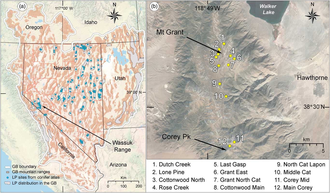
Figure 1. Study region and study area. (a) Great Basin (GB), southwestern USA, showing GB boundary and mountain ranges, distribution of limber pine (LP) in the GB, location of 260 modern limber pine records from the conifer atlas database (Charlet, Reference Charlet1996), and location of the study sites in the Wassuk Range. Basemap from the National Geographic Society. (b) Wassuk Range, Mineral Country, Nevada, showing limber pine stands sampled for dendrochronological and demographic analysis. Basemap from Google Earth Pro.
In the Wassuk Range of west-central Nevada, limber pine currently grows in very sparse stands primarily on north to northeast slopes (Fig. 2a). Scattered across these and other aspects where no live trees occur are remnant deadwood stems, preserved under the dry conditions of the range and testifying to former forests that once grew on these now-treeless slopes (Fig. 2b). We took advantage of this situation to explore the population dynamics and growth of limber pine over the period of record (POR) of available samples, and to investigate relationships with climate variability. We asked the following questions: (1) What primary climate variables correlate with limber pine radial growth and how do interpretations from ring-width-reconstructed paleoclimates compare to other proxies? (2) Has limber pine shifted in elevation and/or aspect over the POR and, if so, what relationship have these shifts had to climate variability? (3) Does evidence exist for climate refugia and, if so, what environmental conditions pertain to these?
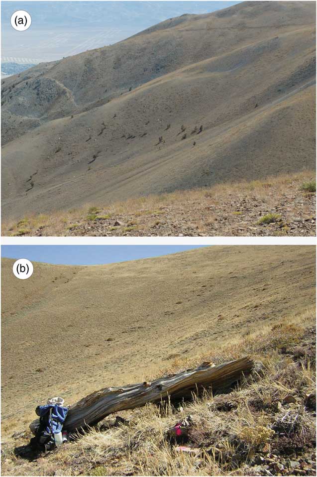
Figure 2. (color online) Limber pine in the Wassuk Range. (a) Live trees grow in sparse, open stands on north and north-east aspect slopes. (b) Relict dead wood stems that occur on many aspects.
METHODS
Study area
The Wassuk Range of west-central Nevada lies within the tectonically active western margin of the GB (Fig. 1). This region is geologically complex due largely to competing forces throughout the Cenozoic and Quaternary of continental plate dynamics related to the Walker Lane fault system versus extensional faulting of the Basin and Range province (Surpless, Reference Surpless2012). A northwest-trending right-lateral strike-slip fault forms a steep escarpment on the eastern side of the range while the west slopes are more gradual (Dong et al., Reference Dong, Ucarkus, Wesnousky, Maloney, Kent, Driscoll and Baskins2014). In the central Wassuk Range, fault blocks consist mostly of Jurassic and Cretaceous granitic rock derived from the Sierran arc and unconformably overlain by Tertiary volcanic and sedimentary rocks (Dong et al., Reference Dong, Ucarkus, Wesnousky, Maloney, Kent, Driscoll and Baskins2014). Slopes of the central Wassuk Range rise 1600–2240 m above adjacent basins, reaching summit plateaus and peaks above 3200 m to the highpoint of Mt. Grant (3440 m). The broad basin to the east of the range contains 120-km2 Walker Lake, a remnant of Pleistocene Lake Lahontan, while the East Fork Walker River runs northward through the basin to the west.
The climate of the Wassuk Range is semiarid and transitional between Mediterranean and Continental regimes. Summers are warm and dry, and winters are cool with sporadic precipitation events. Precipitation in winter derives from remnants of storms originating in the Pacific Ocean. A triple rain shadow, created by the Sierra Nevada, Sweetwater-Bodie Mountains, and Pine Grove Hills, contributes to aridity. Convection storms in summer deliver trace amounts to the meager annual precipitation. Nearby weather stations are in low-elevation basins where conditions differ greatly from those on upland slopes. Values estimated from the PRISM climate model (Daly et al., Reference Daly, Neilson and Phillips1994; Strachan and Daly, Reference Strachan and Daly2017) better represent the high elevations (Table 1).
Table 1. Meteorological data for the Wassuk Range derived from the PRISM Climate Model, 1981–2010 normals (Daly et al., Reference Daly, Neilson and Phillips1994). Values estimated are means across the 12 sample stands (Fig. 1b, Table 3)

Vegetation on the slopes of the Wassuk Range follows typical GB elevational gradation, although shallow soils and semiarid conditions support only sparse growth. Big sagebrush (Artemisia tridentata) steppe communities occur near the base of the range and extend through mid-elevation pinyon-juniper (Pinus monophylla-Juniperus osteosperma) woodlands. High-elevation open slopes have low sage-shrub (Artemisia arbuscula) communities in a sparse mosaic of alpine herbaceous communities comprising grasses, cespitose plants, and barren talus slopes (Bell and Johnson, Reference Bell and Johnson1980). Limber pine occurs as the sole subalpine conifer species in the range. The widely distributed deadwood likely is limber pine despite the fact that the nearest ranges with subalpine conifers contain both limber pine and whitebark pine (Pinus albicaulis). No live whitebark pine has been found in the Wassuk Range despite extensive search and an erroneous report in 1940 (Charlet, Reference Charlet1996). Wood samples from eight dead stems taken in widely separated drainages were identified as limber pine by the USFS Forest Products Lab, Madison, Wisconsin (Wiedenhoft, A., personal communication, 2005, 2013). Widespread fire appears to have been absent due to insufficient fuel, suggesting that relict deadwood has persisted without significant degradation from disturbances other than eventual decomposition.
Field and laboratory methods
On the plateau and slopes from Mt. Grant to Corey Peak, we extracted increment cores from live trees and cores and stem cross-sections from deadwood, sampling all main slope aspects and most major drainages that contained live or dead limber pine (Fig. 1b). Samples spanned the upland elevation range of the species. In the field, we recorded latitude, longitude, elevation, and aspect for all samples. In the laboratory, air-dried increment cores and stem cross-sections were processed using standard dendrochronological techniques (Holmes et al., Reference Holmes, Adams and Fritts1986; Cook and Kairiukstis, Reference Cook and Kairukstis1990). The annual ring sequence of each sample was measured to 0.001-mm accuracy using a Velmex measuring system interfaced with MEASURE J2X measurement software (Consulting Voortech, 2005).
Program COFECHA was used to assess measurement quality and perform cross-dating correlation analyses (Holmes, Reference Holmes1983; Grissino-Mayer, Reference Grissino-Mayer2001). A 10–15-yr cubic smoothing spline (50% frequency cutoff) was employed in COFECHA to maximize series intercorrelation and minimize the number of generated error flags (Krusic and Cook, Reference Krusic and Cook2013). Samples having ambiguous cross-dating features or correlations less than 0.2 were excluded from analysis. Dating was achieved initially by developing a site chronology with reference to local trees and to other limber-pine chronologies from the region we have developed.
To assess change in tree abundance over time, we conducted Webster analyses (Legendre and Legendre, Reference Legendre and Legendre1998, pp. 693–696), using 20-yr paired moving windows, and shifting windows annually across the 3996-yr POR. The database for analysis included inner to outer year dates of all series. Significant differences between windows were evaluated with t-tests, using the Satterthwaite approximation for degrees of freedom to account for heterogeneous variances (Steele and Torrie, Reference Steele and Torrie1980). The t-test evaluates differences in mean number of series in the window 20 yr prior and 20 yr following with annual shifts.
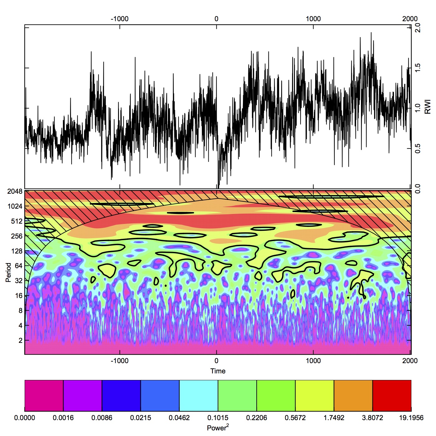
To develop a master chronology for climate reconstruction, we screened the initial chronology to contain only series with correlations ≥0.45. Cross-dating was confirmed by comparing the sample measurement series to bristlecone pine tree-ring chronologies obtained from the International Tree-Ring Data Bank (ITRDB; White Mountains Master ITRDB CA506, Campito Mountain ITRDB CA533, Methuselah Walk ITRDB CA535; ITRDB, 2017–2018) and our own limber-pine chronologies from nearby locations. For analysis with historical and paleoclimatic data, we developed a standardized master chronology with the program ARSTAN v.44h3 (Cook and Krusic, Reference Cook and Krusic2014), using the regional curve standardization method (Esper et al., Reference Esper, Cook and Schweingruber2002) with a 200-yr cubic spline, variance stabilization with 90% n, 50% frequency cutoff, and with a robust bi-weight mean to eliminate ancillary stand factors. To examine low-frequency behavior of the chronology, we decomposed the time series using wavelet analysis into periodic modes and time. We used the Gaussian Morlet wavelet transform in dplR (Bunn, Reference Bunn2008; R Core Team, 2017) and also the Gabor transform, a complex Morlet wavelet, in Mathematica (Wolfram, 2017).
Analysis of growth-climate relationships
To assess climate influences on radial growth during the historic period, we followed methods of Millar et al. (Reference Millar, Westfall, Delany, Flint and Flint2015) to develop a climate dataset using weather station records. The four selected stations were in the general region of the study area, belonged to the NOAA Historical Climate Network (USHCN v2.5; https://www.ncdc.noaa.gov/ushcn/introduction), had the longest PORs, and had the most complete datasets (Table 2), despite that all were at low elevations relative to the study sites. Using principal component analysis, the data from individual stations were combined into a composite record (AD 1895–2017) for mean monthly minimum temperature (Tmin), maximum temperature (Tmax), and annual precipitation. The latter was transformed to water-year precipitation (WYprecip; Oct 1–Sept 30). We also extracted indices of the Atlantic Multidecadal Oscillation (AMO; https://www.esrl.noaa.gov/psd/data/correlation/amon.us.long.data) and of the Pacific Decadal Oscillation (PDO; http://research.jisao.washington.edu/pdo/PDO.latest.txt) for correlation analyses with radial growth.
Table 2. Weather stations providing long-term data used to assess climatic relationships and radial growth in limber pine. Data provided by the Historical Climate Network (USHCN), with periods of record for all stations 1895–2017, National Climate Data Center (www.ncdc.noaa.gov/oa/climate/research/ushcn/).

To further explore water relationships of importance to tree growth, we modeled climatic water deficit (CWD) for the study sites, using a regional water-balance model, the Basin Characterization Model (Flint et al., Reference Flint, Flint, Thorne and Boynton2013), with local data provided by Lorraine Flint (USGS, California Water Science Center). CWD is a measure of moisture availability to plants as indicated by evaporative demand that exceeds available water, and is computed as potential evapotranspiration minus actual evapotranspiration. CWD ranges from zero, when soils are fully saturated, to positive values with no upper limit. Higher values indicate soils that are depleted of water, i.e., water is increasingly unavailable to meet transpirational demands.
Lead cross-correlations were assessed by transfer functions in the time series platform in JMP (SAS Institute, 2015), whereby standardized tree-ring width was the dependent variable and climate variables were the independent variables. Where there were significant lead correlations, we summed the data over 1–4 lead yr. To test relationships of climate variables to standardized annual ring width, we analyzed simple linear correlations as well as nonlinear relationships. For the latter, we conducted a second-order least-squares response-surface model (SAS Institute, 2015) with Tmin, Tmax, and WYprecip, using annual and monthly (and lead yr, where appropriate) measures from the composite climate dataset. The behavior of these variables was evaluated in second-order response models of the form (x + y +...) + (x + y +...)2 in which redundant interactions were omitted. Using stepwise regression, we filtered the model to select only the significant independent variables for further development of a best-fit model for the ring-width data, and evaluated the behavior of these variables in a second-order response-surface model. The behavior of variables included canonical analysis of the model and determining the position of the stationary point, whereby the value of the response neither rises nor falls away from that point (Box and Draper, Reference Box and Draper1987, pp. 323–341; SAS Institute, 2015). Stepwise models were fit by minimizing both the corrected Akaikes Information Criterion and the Schwarz Bayesian Criterion scores (SAS Institute, 2015).
Aspect analysis of contemporary GB limber pines
To assess the importance of north aspects for limber pines beyond the Wassuk Range, we queried a database of GB tree occurrence records developed for the Atlas of Nevada Conifers (Charlet, Reference Charlet1996) and new records contributing to a second edition, currently unpublished. Records specify individual, geo-referenced, native trees sourced from published literature, verified field observations, or herbarium records. We assigned aspect quadrants to each record using ArcGIS and Google Earth Pro. Uniformity of occurrence by aspect was tested with chi square, with equal occurrences by aspect as the null hypothesis.
To assess the influence of sunlight by aspect in the Wassuk Range, we calculated total daily solar radiation with the solar radiation tool in ArcMap (Fu and Rich, Reference Fu and Rich1999). The tool uses aspect and slope from a 30-m digital elevation model to derive a measure of total daily clear-sky radiation (diffuse and direct). We selected the single-day period of August 15 to represent total solar radiation during peak summer heat, a date used in other GB analyses (Van Gunst et al., Reference Van Gunst, Weisberg, Yang and Fan2016; Jeffress et al., Reference Jeffress, VanGunst and Millar2017). We calculated solar loading for all sampled watersheds in the Wassuk Range. Differences in solar radiation sums among aspects were assessed by a mixed-model ANOVA.
RESULTS
Age, aspect, and elevation of limber pine live trees and relict wood
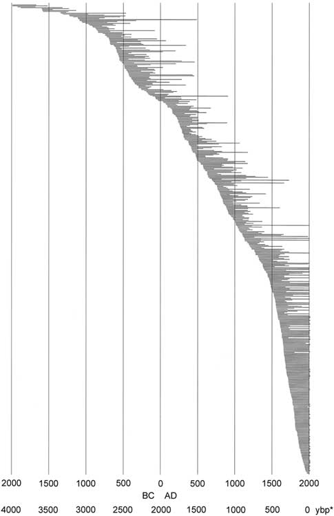
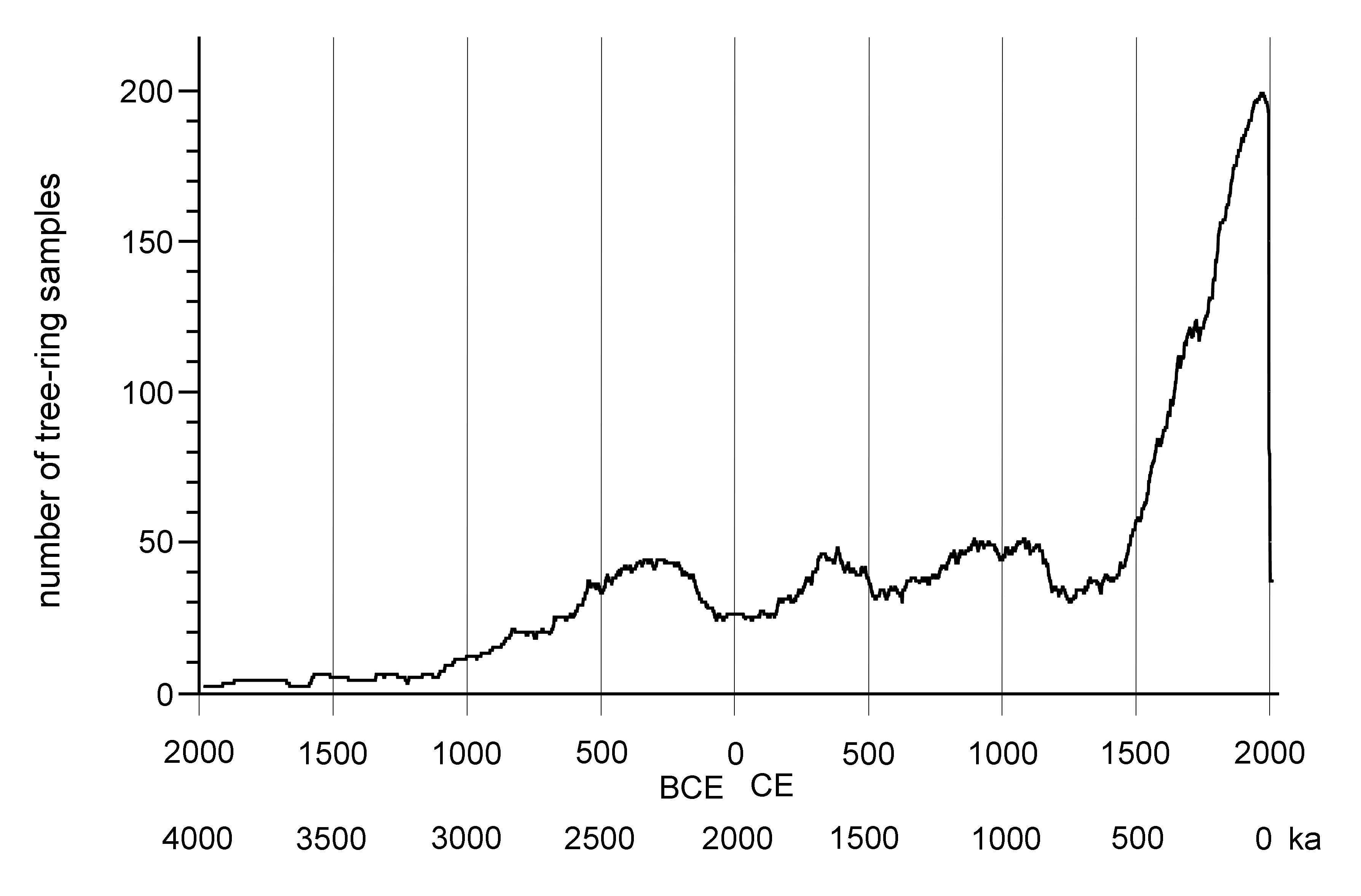
Core and wood samples retrieved from the Wassuk Range yielded 509 dated tree-ring series for the initial chronology (Fig. 3). These series represented 12 watersheds and all primary slope aspects (Table 3). Considering all series and locations together, dates were continuous from the present (outer ring; AD 2013) to 1983 BC (inner ring; two samples), thus extending across 3996 yr without gaps. Verification of a subsample of live trees in 2017 revealed no recent mortality, updating the field record to 4000 yr. Sample depth for all 100-yr intervals except the oldest period (>1100 BC) was at least 10 series/interval and usually many more (Supplemental Figure 1). For the period 1100 BC to 1750 BC, sample depth was 7–9; the oldest interval was represented by four series. Samples that included rings 1000 BC or older (21 series) were distributed across six of the nine drainages of Mt. Grant. The oldest live trees had 988 rings, and the longest deadwood series had 1575 rings. No samples dated older than 1983 BC despite the fact that sample depth was strong in the older intervals, older samples were well-preserved and scattered among locations, and standard chronologies exist that extend to much older dates, providing adequate reference.

Figure 3. Limber pine live and dead tree-ring series ordered chronologically by inside ring date; all dated stems (N=509). *, yr before present (present=AD 2017).
Table 3. Limber pine live trees and deadwood sampled for dendrochronological analysis, Wassuk Range, Nevada, with elevation and age ranges of sampled trees and wood. N, north; W, west; S, south; E, east; NW, northwest; SW, southwest.

1 np indicates no live trees were present in the watershed.
Demographic analyses based on the Webster method revealed significant differences within the last 3100 yr in number of series (abundance of stems; P<0.001), with significant decreases in abundance 100 BC–AD 300, AD 500–600, AD 1250–1300, and AD 1750 (Supplemental Figure 1). Changes in abundance described below were periods of significant differences. Individual series were sorted chronologically by inside ring (Fig. 3 and 4) to highlight trends over time related to tree recruitment. In some cases, especially for deadwood, the center (pith) and/or outer rings were not present due to wood erosion, making exact germination and death dates uncertain. Overall, north-facing slopes had the largest number of stems, live and dead, for all periods except dates older than 1200 BC; the oldest series occurred on westward aspects (Fig. 4). With the exception of that interval, only the north slopes had continuous occurrence of samples. Periods of apparent extirpation, and/or significant decreases in sample depth occurred on the other slope aspects, with synchronies in some periods while not in others. South and west aspect slopes had no samples with pith dates younger than AD 1200; on east slopes an interval of low sample depth (one series) occurred from AD 1150–1450. Low sample intervals occurred at roughly the same time on different aspects: from 350 BC–AD 150 on east aspects (including a gap in the record from 150 BC–AD 100) and north slopes; from 250 BC–AD 200 on south slopes; and from 50 BC–AD 250 on west slopes. A gap in the record on west slopes occurred from 1250 BC–1100 BC. An inflection point of inside rings occurred at ~ AD 1400, with an interval of increased death rates (outside rings) at AD 1600–1700.

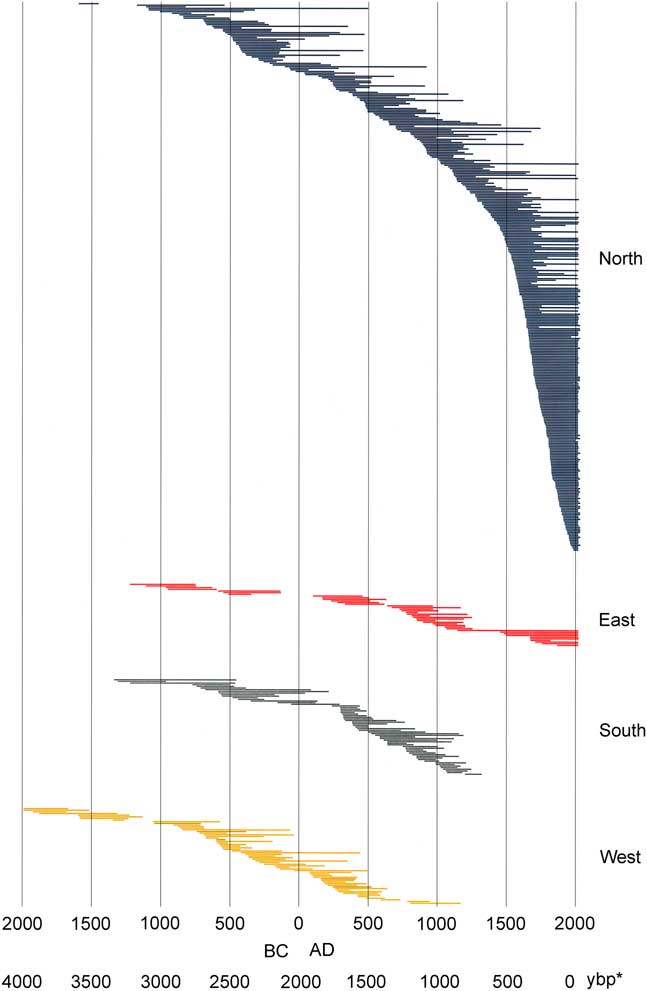
Figure 4. (color online) Limber pine live and dead tree-ring series ordered chronologically by inside ring date and by slope aspect. *, yr before present (present=AD 2017)
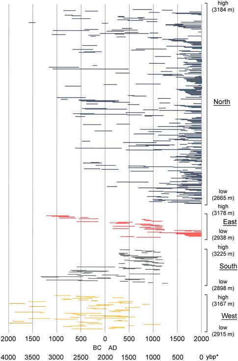
Elevations of live trees and deadwood samples overall extended from 2655–3182 m (Table 3). Live trees and deadwood occurred across the same elevation ranges: overall, sampled live trees extended 54 m lower than deadwood, whereas deadwood extended 12 m higher than live trees; these differences were due only to a few outliers. Patterns of elevation occurrence over time varied by aspect (Fig. 5). On north and west slopes, no trend was obvious; on east slopes, elevations of samples decreased over time (highest, 1200 to 200 BC; lowest elevations, AD 1500 to present); and on the south slopes, elevation of samples increased over time (lowest, 1200 BC to AD 100; highest, AD 250 to 1200). Samples on all aspects had their widest elevation spans during the period from AD 200 to 1200.
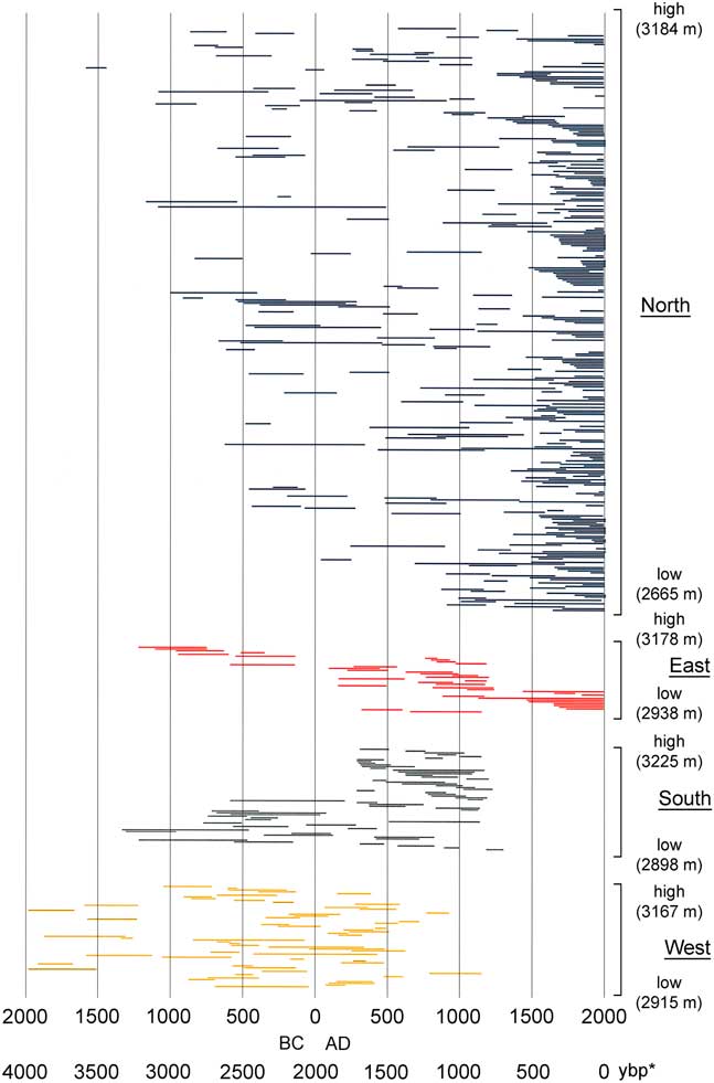
Figure 5. (color online) Limber pine live and dead tree-ring series ordered by aspect and elevation. Within each aspect group, the highest elevation sample is at the top and the lowest elevation sample is at the bottom. Elevation ranges for each aspect group were similar (Table 3). *, yr before present (present=AD 2017)
Trends in radial growth
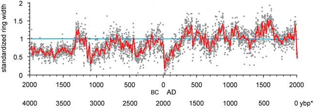
From the initial dated chronology, 290 series had correlations ≥0.45 and were included in the master chronology. Taken together, standardized ring widths showed periods of low-frequency variation with significant power (spectral density; 99% confidence intervals; Fig. 6, Supplemental Figure 2). Episodes equivalent to PDO (32 yr) and AMO (64 yr) periods were significant. Periods of highest magnitude were at about 500 yr and in the 1000–2048 yr range (Supplemental Figure 2). Interannual variation was rather high (s=0.30; s is an estimate of standard deviation) and highly persistent, with significant autocorrelation extending beyond 25 yr. An autoregressive, moving average process fit the data at 2-yr-autoregressive/2-yr moving-average (2, 2), the moving average showed persistence of lower-frequency effects throughout the chronology (Bunn et al., Reference Bunn, Jansma, Korpela, Westfall and Baldwin2013). Excluding the period before ~1100 BC (lower sample depth and variable interseries correlations with the master ), the strongest signal in the POR was an interval of very low growth from 20 BC to AD 150, which was lower than any other period. The second major pattern was low growth in the oldest 40% of the chronology (1100 BC to AD 150) relative to the 3116-yr truncated record, and high growth in the most recent 60% of the chronology (AD 150 to present). Within the recent 1500 yr, periods of low growth occurred at AD 600–800, 900–1050, 1150–1450, and 1650–1960. A short spike of high growth occurred from AD 1960–1980, followed by a rapid decline in growth during the last two decades. Growth in this most recent period was lower than at any time in the past 3116 yr except during the lowest growth interval of 20 BC to AD 150.

Figure 6. (color online) Standardized ring widths for Wassuk Range limber pine chronology across 3996 yr. To show low-frequency variation, smoothing was done with a cubic spline with lambda=10,000 (gray curve; SAS 2015). *, yr before present (present=AD 2017)
Ring-width-climate relationships relative to the instrumental period
Best-fit models of standardized ring widths to climate with stepwise regressions yielded R ≥ 0.72 and a model excluding mid-frequency indices had R 2≥0.55 (P<0.0001; Table 4). The highest individual correlation of radial growth was with the AMO (R=-0.52) and with CWD (R=-0.47). For the instrumental period (~AD 1900–present), CWD values corresponded to patterns of the AMO, with a period of low values at AD 1900–1920 and AD 1965–1990; intervals of high growth and a plateau with mid-range values at AD 1930–1965; and highest values from AD 1990 to present (Supplemental Figure 3). The periods of high CWD corresponded to low values of WYprecip and relatively high Tmax and Tmin, and to intervals of low ring width. Significant negative correlations also occurred with lead-year annual (calendar) Tmin, July and August Tmin, and lead-year July Tmax, respectively (all P < 0.0001). A strong positive correlation occurred with lead WYprecip (R=0.46); other significant positive correlations occurred with July and September precipitation (all P<0.0001). Interaction plots indicated that, under low values of July precipitation, increases in August Tmin decreased growth, whereas there was no change under high values of precipitation and similarly for low values of CWD and PDO indices relative to August Tmin. The response surface was a saddle point and critical values for dependent variables were outside their data range, as was the predicted value at solution for ring width (Box and Draper, Reference Box and Draper1987, p. 340), suggesting that the climate over the POR (past 120 yr) did not exceed the adaptive limits for growth.
Table 4. Model correlations and climate variables included in the best-fit stepwise regression analyses for radial ring-width models, based on the date range 1893 BC–AD 2016. Squared multiple correlation coefficients are given for models with and without low-frequency indices included. Simple correlations with variables not included in the full model are also shown.
a Models with the low-frequency indices included.
b Models with low-frequency indices omitted.
Aspect analysis of contemporary GB limber pines
Data from the Nevada conifer atlas contained 260 limber pine occurrence records from 49 mountain ranges. Of these, 63% occurred on northward aspects (north quadrant), a highly significant (P≪0.0001) deviation from equal representation by quadrant. Remaining records were relatively evenly distributed on the other three quadrants (14% east; 13% west; and 10% south); 11 occurrence records were on flat ground. Upland north slopes, particularly the north and northeast octants, in the Wassuk Range that currently support limber pines were estimated to receive significantly lower solar input than other aspects P<0.0001; Table 5). East-facing slopes received near-mean loading, while south and west aspects received significantly higher than mean loading (P<0.05).
Table 5. Solar radiation estimated for limber-pine upland slopes in the Wassuk Range, Nevada, averaged over slope octants. Area assessed included the 12 study watersheds. Units are watts per square meter. N, number of digital elevation model tiles representing limber pine habitat on these slopes.

DISCUSSION
Climate variability over 4000 yr and relationship to radial growth
Correlations of limber pine in this study with modern climate are similar to those we have calculated from shorter chronologies (last 250 yr; Millar et al., Reference Millar, Westfall, Delany, Flint and Flint2015), and differ somewhat from responses of other subalpine pine species in the region. Bristlecone pine growing in the GB through the last millennium generally responded to precipitation at lower tree line and temperature at upper tree line (Hughes and Funkhouser, Reference Hughes and Funkhouser2003; Salzer et al., Reference Salzer, Hughes, Bunn and Kipfmueller2009, Reference Salzer, Bunn, Graham and Hughes2014). Scuderi (Reference Scuderi1993) reported strong correlations for foxtail pine (Pinus balfouriana) growing in the eastern Sierra Nevada with high temperatures but not with precipitation. The same species growing near upper tree line in relatively mesic sites of the Sierra Nevada responded more similarly to limber pine in high radial growth with high lead winter precipitation but differed in having positive growth with high summer temperatures (Graumlich, Reference Graumlich1993). At the most xeric site, however, foxtail pine response resembled limber pine in having minimum growth rates when precipitation was below average and temperature was above average.
Millennial- and centennial-scale variability has been studied extensively for the GB using a variety of approaches (Grayson, Reference Grayson2011 for overview). We summarize major climate periods of the mid-late Holocene and compare these to patterns in limber pine radial growth. Multiple independent proxies document the Middle Holocene, ~7.5–4 ka, as an extensive dry, hot interval across most of the GB (Grayson, Reference Grayson2011). Lake levels were low or lakes were desiccated, arid-adapted flora and fauna expanded, and the bristlecone pine tree line rose by 153 m in the White Mountains, interpreted as a 1.5°C warming relative to the mid-twentieth century (LaMarche, Reference LaMarche1973) and a 2.8–7.2°C warming based on Pyramid Lake surface elevations (Benson et al., Reference Benson, Kashgarian, Rye, Lund, Paillet, Smoot, Kester, Mensing, Meko and Lindstrom2002).
The shift to cooler and wetter conditions commonly associated with the Neoglacial started ~5000 yr ago, at 4700 cal yr BP in the eastern GB (Ruby Marsh; Thompson, Reference Thompson1992), ~4400 and 3400 cal yr BP at Blue Lakes (Louderback and Rhode, Reference Louderback and Rhode2009), and ~4000 cal yr BP in the Snake Range, where a 1.5°C decline from peak Middle Holocene warmth was interpreted across the subsequent millennium (Reinemann et al., Reference Reinemann, Porinchu, Bloom, Mark and Box2009). Wetter conditions were interpreted from increases in lake levels: Owens Lake began to freshen ~3600 yr ago (Benson et al., Reference Benson, Lund, Smoot, Kashgarian and Burdett2001) and Pyramid Lake did the same ~3500 yr ago (Benson et al., Reference Benson, Kashgarian, Rye, Lund, Paillet, Smoot, Kester, Mensing, Meko and Lindstrom2002). In the Sierra Nevada, notable glaciations occurred at 3900, 3200, and 2800 cal yr BP (Konrad and Clark, Reference Konrad and Clark1998; Bowerman and Clark, Reference Bowerman and Clark2011). High stands are recorded for lakes in the western GB, including Mono Lake at ~3700 cal yr BP (Stine, Reference Stine1990) and Walker Lake, adjacent to the Wassuk Range, at ~3400 cal yr BP (Adams, Reference Adams2007).
Against this background and without records to verify, we speculate that limber pine extent was minimal or absent in the Wassuk Range during the hot, dry conditions of the Middle Holocene. Any trees existing then would likely have had very slow radial growth, and (per discussion about refugia below) be restricted to north aspects. The shift to Neoglacial cooler and wetter conditions likely triggered expansion of limber pines across the slopes of the Wassuk Range (or [re]colonization into the range) to the point when our records begin. Cold conditions would constrain growth in limber pine, despite ample precipitation.
Increasing aridity in the central GB began ~2800 and continued to ~1850 cal yr BP (Tausch et al., Reference Tausch, Nowak and Mensing2004; Mensing et al., Reference Mensing, Sharpe, Tunno, Sada, Thomas, Starratt and Smith2013), defining the Late Holocene Dry Period. This multi-century dry interval has been documented at many locations and with multiple proxies (Mensing et al., Reference Mensing, Sharpe, Tunno, Sada, Thomas, Starratt and Smith2013). Severe, prolonged drought is indicated by lakes, rivers, and marshes becoming desiccated or reaching low stands (e.g., Walker Lake [Adams, Reference Adams2007], Mono Lake [Stine, Reference Stine1990, Reference Stine1994], and Pyramid Lake [Mensing et al., Reference Mensing, Benson, Kashgarian and Lund2004, Reference Mensing, Smith, Norman and Allan2008]), and by expansion of dry-adapted vegetation. The most severe drought effects are recorded for the western GB (Mensing et al., Reference Mensing, Sharpe, Tunno, Sada, Thomas, Starratt and Smith2013). Temperatures during the LHDP were not obviously anomalous relative to the Neoglacial; no evidence exists for unusual warmth, given the continuing occurrence of glacial advances in the western and eastern parts of the region (Reinemann et al., Reference Reinemann, Porinchu, Bloom, Mark and Box2009; Bowerman and Clark, Reference Bowerman and Clark2011).
The extended multi-century period of low radial growth in limber pine (1100 BC to AD 150) corroborates aridity of the LHDP. Extreme low growth (20 BC to AD 150) in limber pine occurred at a time when other proxies also showed extreme dry conditions, as evidenced in Toiyabe, Toquima, and Monitor Ranges geomorphology (Miller et al., Reference Miller, House, Germanoski, Tausch and Chambers2004), Kingston Meadow, Toiyabe Range, sediments, (Mensing et al., Reference Mensing, Smith, Norman and Allan2008), Pyramid Lake vegetation (Mensing et al., Reference Mensing, Benson, Kashgarian and Lund2004), and surface elevations of Walker Lake (Adams, Reference Adams2007) and Mono Lake (Stine, Reference Stine1990).
A short, cool, wet period intervened between the end of the LHDP and the start of the next dry interval, the MCA (Stine, Reference Stine1994). Two severe and persistent droughts are recorded for the western GB MCA, at AD 900–1100 and AD 1200–1350 (Stine, Reference Stine1994), documented by low lake and stream levels (Stine, Reference Stine1990; Mensing et al., Reference Mensing, Benson, Kashgarian and Lund2004, Reference Mensing, Smith, Norman and Allan2008; Adams, Reference Adams2007), increase in arid-adapted vegetation (Mensing et al., Reference Mensing, Smith, Norman and Allan2008, Reference Mensing, Sharpe, Tunno, Sada, Thomas, Starratt and Smith2013), and other proxies. Anomalous warmth is interpreted from high-elevation conifer tree rings in the Sierra Nevada (Graumlich, Reference Graumlich1993; Scuderi, Reference Scuderi1993) and from an anomalous mixed-conifer forest that grew at high elevation during this period, with modeled temperatures warmer (+3.2°C) and drier than the mid-twentieth century (Millar et al., Reference Millar, King, Westfall, Alden and Delany2006). Separating the two centennial-scale MCA droughts was a 50-yr pluvial period, interpreted from Walker Lake records (Hatchett et al., Reference Hatchett, Boyle, Putnam and Bassett2015).
Limber pine growth paralleled climate trends of this time period, with an exception. Growth was above average from AD 200–700, corroborating return of wetter, cool conditions following the LHDP, as indicated by a high stand at Walker Lake (Adams, Reference Adams2007). An interval from AD 625–750, when limber pine had low growth, is not explained by climate indicators from other records. Low growth episodes characterized the two drought periods of the MCA, and high growth characterized the short mid-MCA pluvial. These patterns differ somewhat from the detailed analyses of bristlecone pine growth for this period (LaMarch, Reference LaMarche1974), particularly that the more northerly Wassuk Range is less influenced by strong monsoonal variability that the White Mountains.
Following the MCA, the global Little Ice Age (LIA) brought persistent cold and wet conditions to the GB from ~AD 1400 to 1920. These conditions are indicated by many proxies, including, for the western GB, tree line and tree rings (LaMarche, Reference LaMarche1974; Graumlich, Reference Graumlich1993; Scuderi, Reference Scuderi1993; Feng and Epstein, Reference Feng and Epstein1994; Lloyd and Graumlich, Reference Lloyd and Graumlich1997), glacial advances in the western and central GB (Osborne and Bevis, Reference Osborne and Bevis2001; Bowerman and Clark, Reference Bowerman and Clark2011), and increases in lake and river levels (Walker Lake levels might be misleading at this time due to diversions of the input river; Stine, Reference Stine1990; Mensing et al., Reference Mensing, Sharpe, Tunno, Sada, Thomas, Starratt and Smith2013). Decreases in summer minimum temperature of 0.2–2°C and increases in winter precipitation of 3–26 cm compared to modern times have been interpreted to explain glacial conditions (Bowerman and Clark, Reference Bowerman and Clark2011). Rapid cooling began ~AD 1600, with maximum cold ~AD 1700–1900; summers significantly cooler than the present persisted to AD 1930 (Feng and Epstein, Reference Feng and Epstein1994).
In the case of the LIA centuries, limber pine growth showed two distinct periods, dividing the interval by high growth (AD 1350–1600) and near-mean growth (AD 1650–1930). Given the climate responses of limber pine, this could be interpreted as the increase of moisture with cool temperatures of the early LIA centuries favoring growth, whereas intense cold after AD 1600 reduced growth, despite adequate precipitation, a response seen earlier in the record. In the White Mountains, the early period is marked by relatively strong growth at the lower border of bristlecone pine, interpreted as persistent moisture, whereas the latter period, like limber pine, had low growth, interpreted as cool and dry (LaMarche, Reference LaMarche1974).
Following the LIA, temperatures in the western GB warmed gradually in the early twentieth century to a mid-century plateau, then rapidly increased in the late century and early twenty-first century (Moritz et al., Reference Moritz, Patton, Conroy, Parra, White and Beissinger2008). Despite warmth, conditions remained relatively wet (Graumlich, Reference Graumlich1993), although multiyear droughts have punctuated the past 130 yr in the southwestern GB (Millar et al., Reference Millar, Westfall and Delany2007). Limber pine responded with increased growth as the twentieth century warmed and remained wet. Subsequent to an extreme wet period in the 1980s, increasing temperatures and drought, from the spline fit, appear related to the second largest continuous decline in limber pine growth in the record.
Shifts and persistence of limber pine by aspect and elevation and relationship to climate
Whereas radial-growth variability corresponded with trends in centennial climate as outlined above, patterns of limber-pine demography were far less coherent. We first consider potential biases of inner and outer dates for our series. Despite that recruitment and death dates were often not precise due to wood erosion, large sample depth throughout the record, and the coarse scale (centennial and millennial) of analysis should provide for an accurate picture of pine dynamics at the watershed scale over the last 4000 yr. Further, seedling establishment is much more sensitive to climate than tree death at these elevations (LaMarche and Mooney, Reference LaMarche and Mooney1967; Elliott, Reference Elliott2012; Barber, Reference Barber2013), and birth dates are more reliable in our record than death dates. Other biases in the record might include removal of wood through differential decomposition or by fire. North aspects, however, would be expected to have highest decomposition rates, yet these slopes retained the largest number of stems, except in the oldest interval when preservation limits might have been reached. Preservation of old wood on all slopes testifies to the lack of landscape fire.
Low correspondence of demographic and radial-growth trends might relate to differences in climate responses between seedlings and mature trees, as reported also for foxtail pine (Lloyd and Graumlich, Reference Lloyd and Graumlich1997; Bunn et al., Reference Bunn, Waggoner and Graumlich2005). Limber-pine seedling associations are quite similar to those for radial growth (Millar et al., Reference Millar, Westfall, Delany, Flint and Flint2015) and include positive correlations with water-year, summer, and autumn precipitation; and negative associations with annual and summer maximum temperatures and CWD. These did not, however, provide useful insight into demographic patterns. For instance, one expectation was that north aspects, with lower solar loading, lower temperatures, longer snow retention, and higher soil moisture than other aspects, would favor pine establishment and persistence during warm, dry periods relative to cold, wet intervals. Conversely, during cold periods, slopes that are warmer and drier would support pine stands. This was not the case in the Wassuk Range, as pines appeared to have flourished on all aspects, including the north, during the coldest and wettest part of the Neoglacial (i.e., before 2800 ka). Similarly, during the cold LIA, north and east slopes supported limber pines, whereas no pines grew on south and west aspects. The expectation that cooler, wetter north aspects would favor pine abundance during arid and/or warm intervals was also not supported in the Wassuk data. During the hot, dry LHDP, pines recruited and persisted on all aspects; during the warm, dry MCA, pines occurred on north, east, and south aspects. An influence of warm and dry conditions might be a lack of pine recruitment on west aspects at the start of the MCA, with eventual extirpation.
Expectations about elevation and climate also were not supported by limber-pine stand dynamics. We found no evidence to support the expectation that with warming and/or drying climates pines would shift up in elevation, as has been found for other pines in the GB, including foxtail pine (Graumlich, Reference Graumlich1993; Scuderi, Reference Scuderi1993; Lloyd and Graumlich, Reference Lloyd and Graumlich1997) and bristlecone pine (LaMarche, Reference LaMarche1973; Salzer et al., Reference Salzer, Bunn, Graham and Hughes2014). In that several periods in the last 4000 yr have been warmer and drier than present, including the LHDP and MCA, we expected to find, but did not, remnant wood at elevations above the current upper tree line. Ample area on the slopes and broad plateau above the current upper tree line exists in the Mt. Grant region, and there is no obvious reason why wood would not be preserved there. Further, if pines grew during the Middle Holocene, we expect they would have grown at higher elevations, as bristlecone pine famously did in the White Mountains, where the tree line advanced 150 m upward (La Marche, Reference LaMarche1973). In the Wassuk case, total stem erosion might have occurred for trees that existed prior to 2000 BC. Similarly, although records of live limber pines growing in extra-marginal low-elevation ravines throughout the GB (Millar et al., Reference Millar, Charlet, Westfall, King, Delany, Flint and Flint2018) suggest that the species might have moved downslope during earlier periods, decomposition in these wet sites likely removes evidence.
A further expectation is that upward shifts in the elevational range during warming climates would be more likely on drier slopes (south, west) than wetter slopes (north, east), while the converse would be expected during cool, wet periods. Limber pines in the Wassuk Range, however, showed no consistency with elevation and climate. On north slopes, pines occupied the full elevation range throughout the 4000-yr record; a similar pattern occurred on the west slope with the exception that pines were extirpated by ~1100 ka. On south and east slopes there was a trend of shifting elevations over time, but the patterns were not consistent with climate. South slopes had pines at lowest elevations during the hot, dry LHDP, and occupied the full elevation range during the hot, dry MCA; pines on east slopes generally declined over the millennia, with the broadest elevation range distribution during the MCA.
The single climate influence consistent with expectations of pine response were the extirpations on the east, south, and west slopes that corresponded with warm, dry conditions of the MCA. On west slopes, pines were not reproducing during this period, and most trees had been extirpated by the beginning of the MCA. Pines persisted longer on south aspects but had extirpated 150 yr before the end of the MCA, by ~AD 1200. On east slopes, pines did not reproduce at this time, although mature trees persisted, but, unlike the south and west aspects, recruitment began again on east slopes during the cool, wet LIA, and at low elevations, following expectations.
The relatively poor power of climate to explain stand dynamics suggests that other influences affect long-term demographics. At this scale, lack of seed source and long dispersal distances could override climate in determining presence or absence of forests. South and west slopes in the Wassuk Range occur within large watersheds currently barren of pine forests. Seed dispersal and germination in limber pine is assisted by the bird Clarks’ nutcracker (Nucifraga columbiana), which carries and caches limber pine seeds. While the birds can fly more than 20 km, they generally do not cache seeds where pines do not occur (Lorenz et al., Reference Lorenz, Sullivan, Bakian and Aubry2011). A further obstacle for seedling establishment on treeless slopes is the requirement of pine species for ectomycorrhizal fungi (EMF) in the soil, without which seedlings cannot establish or persist (Smith and Read, Reference Smith and Read2008). In moist environments seeds can germinate without EMF, but seedlings cannot grow beyond a few years without their symbiotic fungi (Collier and Bidartondo, Reference Collier and Bidartondo2009). Seedling survival without EMF in harsh environments is likely to be even more limited, and in semiarid subalpine regions fruiting of fungi is rare and ectomycorrhizal inoculum is restricted to spore banks that are only found in areas around live pines (Bidartondo et al., Reference Bidartondo, Baar and Bruns2001). Although EMF spores might persist for years to decades (Bruns et al., Reference Bruns, Peay, Boynton, Grubisha, Hynson, Nguyen and Rosenstock2009), eventually they are likely to be depleted, and colonization of EMF into treeless sites would be expected to be slow, requiring stepping stones of live pines for dispersal.
Poor seed dispersal and absence of EMF might explain not only a lack of pine recolonization on south and west slopes in the LIA, but also why east slopes did recolonize. East slopes in the Wassuk Range most often occur in watersheds of dominant north and northeast orientations, and thus are adjacent to locations that retained pines. The persistence of pines in abundance on north slopes during unfavorable climate periods might also relate to EMF persistence and seed availability. Deeper soils on north slopes (Toy et al., Reference Toy, Foster and Renard2002) could improve chances for seedling establishment and persistence, leading to higher stand densities. This, in turn, would translate to greater and persistent seed availability and retention of EMF spore banks. These factors could overwhelm climatic forcing.
The role of factors other than climate in limiting the location and timing of forest establishment is suggested from other limber-pine studies in the western GB. The only evidence for recruitment above the current tree line in the past 130 yr dated to one pulse in the late-twentieth century (Millar et al., Reference Millar, Westfall, Delany, Flint and Flint2015). The locations of recruitment occurred only in close proximity to existing live stands despite widespread pine habitat. Similarly, late-twentieth-century pulses of bristlecone pine recruitment occurred in a limited number of clusters above tree line in the White Mountains and near live stands (Salzer et al., Reference Salzer, Bunn, Graham and Hughes2014).
Beyond the role of seed availability and proximity, establishment of seedlings that persist into mature trees in subalpine species has been shown in several studies in western North America to have episodic nature (Millar et al., Reference Millar, Westfall, Delany, King and Graumlich2004; Bunn et al., Reference Bunn, Waggoner and Graumlich2005; Elliott, Reference Elliott2012; Salzer et al., Reference Salzer, Bunn, Graham and Hughes2014; Conlisk et al., Reference Conlisk, Castanha, Germino, Veblen, Smith and Kueppers2017). Although correlations between recruitment and climate often emerge at the annual-to-decadal scale, relative to longer timeframes, irregular and infrequent mature tree age groups in upper tree line zones testify to the complex factors that mediate establishment of seedlings and persistence of mature trees in long-lived subalpine pines (Lloyd and Graumlich, Reference Lloyd and Graumlich1997).
CONCLUSIONS: IMPLICATIONS FOR NORTH SLOPES AS REFUGIA
The persistence of limber pine forests on north aspects of the Wassuk Range across 4000 yr of climate variability prompts the possibility that these slopes have acted as long-term refugia. Abundant remnant wood further suggests that forests were relatively dense on north slopes. The existence of abundant north-slope habitat appears to be more important in providing resilience to climate change than elevation gradients in this semiarid mountain range.
Dobrowski (Reference Dobrowski2011) outlined a theoretical framework for terrain-based climate refugia in temperate mountain landscapes, emphasizing that, for refugia to exist and persist, micro-climatic processes must be decoupled from regional trends, otherwise refugia would be short-lived (see also Hampe and Jump, Reference Hampe and Jump2011). Our analyses corroborate reports wherein terrain influences appear to promote decoupling on north aspects, supporting cool-adapted conifers through the maintenance of appropriate temperature and water relations for persistence despite changing climates around them. Significantly lower solar loadings estimated for north slopes of the Wassuk Range translate to lower temperatures, which in turn promote longer snow retention (Coughlan and Running, Reference Coughlan and Running1997). Persistent snow affords north slopes more soil moisture in long, dry summers, decoupling these environments from regional climate means. Greater soil development on north slopes and feedbacks with increased vegetation (Toy et al., Reference Toy, Foster and Renard2002) would improve the chances for conifer establishment and persistence.
Lending support to the proposal that north slopes are refugial was the greater frequency on north aspects than others of contemporary (live) limber pines across 49 mountain ranges of the GB relative to other aspects. Beyond limber pine, data assessed from the Nevada conifer atlas (Millar et al., Reference Millar, Charlet, Westfall, King, Delany, Flint and Flint2018 indicate that 44% of 1393 records for 15 upland conifers across 122 Nevada mountain ranges occur on north-quadrant slopes, again a significantly greater frequency than expected. North aspects appear to have refugial characteristics important for many montane conifers in warm, semiarid regions such as the GB, where water availability as well as temperature is limiting (Dobrowski, Reference Dobrowski2011; Serra-Diaz et al., Reference Serra-Diaz, Scheller, Syphard and Franklin2015; Gentili et al., Reference Gentili, Baroni, Caccianiga, Armiraglio, Ghiani and Citterio2015). North-slope environments, especially those where upland conifers at present grow in semiarid mountains, deserve priority attention in vulnerability modeling and climate-adaptation planning.
ACKNOWLEDGMENTS
We thank Toni Lyn Morelli (USGS, NE Climate Science Center, Amherst, Massachusetts) and Chrissy Howell (USFS, Pacific Southwest Research Station, Albany, California) for reviews of early versions of the manuscript, and Lorraine Flint (USGS, California Water Science Center, Sacramento, California) for providing geo-referenced cumulative water deficit data for our study region. Many thanks to Johnny Peterson (US Army, Hawthorne Army Depot, Hawthorne, Nevada) and the US Army for providing access to the Mt Grant area of the Wassuk Range and permission to conduct studies on Army land. We thank journal associate editor, Dr. Patrick Bartlein, and external reviewers Dr. Scott Mensing and an anonymous reviewer for their careful reading of the submitted manuscript and constructive comments for the revision.
SUPPLEMENTARY MATERIAL
To view supplementary material for this article, please visit https://doi.org/10.1017/qua.2018.120