


INTRODUCTION
The Late Pleistocene and Holocene paleoenvironmental history of Alaska's Kenai Peninsula (Fig. 1) has long been of interest to geologists and climate scientists (e.g., Cooper, Reference Cooper1942; Karlstrom, Reference Karlstrom1964) due to the region's multi-phased deglaciation (Reger et al., Reference Reger, Sturmann, Berg and Burns2007), spatially and temporally complex transition from tundra to mixed coastal forest (Anderson et al., Reference Anderson, Kaufman, Berg, Schiff and Daigle2017), and sensitivity to synoptic patterns of ocean and atmospheric variability (Bailey et al., Reference Bailey, Klein and Welker2019) and modern climate change (Hayward et al., Reference Hayward, Colt, McTeague and Hollingsworth2017). In recent decades, the development of increasingly sophisticated methods for studying past environments has enhanced our ability to interpret paleoclimate datasets from southern Alaska. For example, developments in our understanding of oxygen isotope systematics and proxy systems have yielded numerous reconstructions of past hydroclimatic change inferred from lake sediment archives in the Kenai Peninsula and surrounding region (e.g., Schiff et al., Reference Schiff, Kaufman, Wolfe, Dodd and Sharp2009; Jones et al., Reference Jones, Wooller and Peteet2014, Reference Jones, Anderson, Keller, Nash, Littell, Wooller and Jolley2019; Broadman et al., Reference Broadman, Kaufman, Henderson, Berg, Anderson, Leng, Stahnke and Muñoz2020).
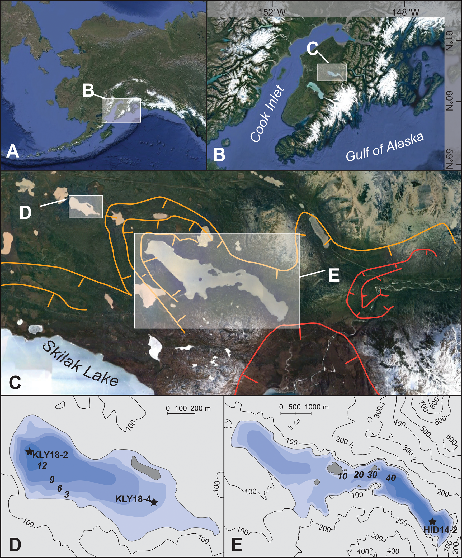
Figure 1. (A) Location of the Kenai Peninsula in Alaska; (B) location of the Hidden Lake and Kelly Lake region of the Kenai lowlands; (C) glacier margins during the Skilak (orange) and Elmendorf (red) stades of the Naptowne glaciation (Reger et al., Reference Reger, Sturmann, Berg and Burns2007), with the location of Kelly (D) and Hidden (E) Lakes indicated; (D) bathymetric map of Kelly Lake; and (E) bathymetric map of Hidden Lake; (D) and (E) show locations of sediment cores discussed in the text. Satellite images from Google Earth.
However, interpreting these datasets remains a challenge because of the many variables that can influence lake water oxygen isotope composition, such as the source of precipitation (e.g., Jones et al., Reference Jones, Wooller and Peteet2014), the balance between precipitation and evaporation (e.g., Anderson et al., Reference Anderson, Abbott, Finney and Burns2007), and the hydrological setting of the lake (e.g., Anderson et al., Reference Anderson, Birks, Rover and Guldager2013). Because these oxygen isotope based reconstructions must attempt to distinguish among these varied influences, many of these studies feature multi-pronged approaches, such as analyzing data from multiple climate proxies (e.g., Broadman et al., Reference Broadman, Kaufman, Henderson, Berg, Anderson, Leng, Stahnke and Muñoz2020) or evaluating the reproducibility of proxy data from multiple, neighboring lakes (e.g., McKay and Kaufman, Reference McKay and Kaufman2009; Krawiec et al., Reference Krawiec and Kaufman2014). Studies in other regions have demonstrated the utility of interpreting lacustrine oxygen isotope data alongside hydrologic and isotope mass balance modeling to constrain the roles of various constituents of a lake's hydrologic budget (e.g., Gibson et al., Reference Gibson, Prepas and McEachern2002; Steinman et al., Reference Steinman, Rosenmeier, Abbott and Bain2010; Lacey and Jones, Reference Lacey and Jones2018). These studies, which combine multiple lines of evidence and multiple modes of analysis, are often able to discern the influences of climate and environmental change recorded in proxy datasets, demonstrating the efficacy of these approaches for reconstructing paleoenvironmental conditions.
In southern Alaska, the increasing sophistication and nuance of recently published paleoclimate reconstructions builds on foundational studies that initially demonstrated the interconnectedness of environmental and climate change in the region. For example, Ager (Reference Ager and Wright1983) first showed that Late Pleistocene and Holocene climate changes in the Kenai Peninsula were accompanied by pronounced shifts in vegetation communities by analyzing pollen in a sediment sequence from Hidden Lake. The transition between glaciolacustrine sediments and gyttja at this site has also been used to constrain the timing of the retreat of glaciers that emanated from the Kenai Mountains and discharged into Hidden Lake during the Pleistocene–Holocene transition (Reger et al., Reference Reger, Sturmann, Berg and Burns2007). However, these environmental changes are constrained by a radiocarbon chronology consisting of only four ages over ca. 15,000 years, all of which were derived from bulk sediment samples (Ager, Reference Ager and Wright1983). In recent decades, studies have shown that bulk sediment samples incorporate old carbon and can yield ages several millennia older than those from macrofossils collected in the same stratigraphic horizon (Grimm et al., Reference Grimm, Maher and Nelson2009), and technological advances in accelerator mass spectrometry have permitted the analysis of smaller samples than was previously possible (Santos et al., Reference Santos, Moore, Southon, Griffin, Hinger and Zhang2007). These advances in our knowledge of radiocarbon, coupled with advances in our ability to analyze and interpret paleoenvironmental data, suggest that re-examining foundational studies (e.g., Ager, Reference Ager and Wright1983) may improve our insights into deglacial and Holocene climate and environmental change on the Kenai Peninsula.
To investigate late glacial and Holocene conditions along the mountain front of the eastern Kenai lowlands, we have developed new multi-proxy paleoclimate datasets from neighboring Hidden and Kelly lakes (Fig. 1C–E). We revisit the foundational pollen record from Hidden Lake (Ager, Reference Ager and Wright1983) and revise the late glacial and Holocene chronology of deglaciation and vegetation change in this region, which we interpret alongside new sedimentological data from this site. We also present Holocene diatom oxygen isotope, diatom assemblage, macrofossil, and sedimentological datasets from Kelly Lake, and use a simple hydrologic and isotope mass balance model to support and quantitatively constrain our interpretations of the diatom oxygen isotope dataset. In particular, we use this modeling approach to investigate the role of groundwater inflow to Kelly Lake during different time periods by providing ranges of plausible values for the other major components of the Kelly Lake hydrological system (precipitation rate, evaporation rate, and the isotope composition of precipitation and groundwater). The simplicity of the modeling framework is useful for constraining the drivers of large hydrologic and isotopic changes at Kelly Lake, because we consider only the most dominant influences on the hydrological budget.
Our findings demonstrate the importance of groundwater in the hydrologic budget at this site, suggesting that climate-driven changes in groundwater inflow can have a profound influence on lake water isotope values. Furthermore, by using varied sedimentological, biological, and geochemical proxy datasets from multiple lakes, coupled with mass balance modeling, we demonstrate the potential of such efforts in creating a multi-faceted reconstruction of paleoenvironmental change.
Study area and regional climate
The Kenai Peninsula is located in south-central Alaska, bordered by Cook Inlet and the Gulf of Alaska (Fig. 1A, B). The Kenai Mountains occupy the southeastern portion of the peninsula and act as a barrier to storms traveling from the North Pacific Ocean, creating a rain shadow effect in the Kenai lowlands to the northwest. Mean annual temperature at the Kenai Moose Pens SNOTEL site was 2.7°C, mean annual rainfall was 47.2 cm, and mean annual snow-water equivalent was 11.4 cm between 1995 and 2019 (National Water and Climate Center, https://www.nrcs.usda.gov/wps/portal/wcc/home/). The majority of precipitation in the Kenai Peninsula occurs from November to March (Fig. 2A), when the Aleutian Low atmospheric pressure cell (AL) strengthens and moves eastward, as opposed to spring and summer months when it weakens and moves westward (Overland et al., Reference Overland, Adams and Bond1999). These seasonal changes in precipitation are accompanied by changes in temperature and the oxygen isotope composition of precipitation (δP) (Fig. 2A), where the summer months are warmer, with higher δP values. Precipitation-weighted seasonal average δP measured in Anchorage are −14.5‰ for summer and −20.7‰ for winter, and −17.7‰ annually (Bailey et al., Reference Bailey, Klein and Welker2019) (Fig. 2A). Both seasonal and interannual shifts in average storm trajectories associated with AL variability can also influence δP (Berkelhammer et al., Reference Berkelhammer, Stott, Yoshimura, Johnson and Sinha2012; Porter et al., Reference Porter, Pisaric, Field, Kokelj, deMontigny, Healy and LeGrande2014). These interannual and longer-term AL fluctuations superimpose an isotope imprint on the average seasonal change in δP.
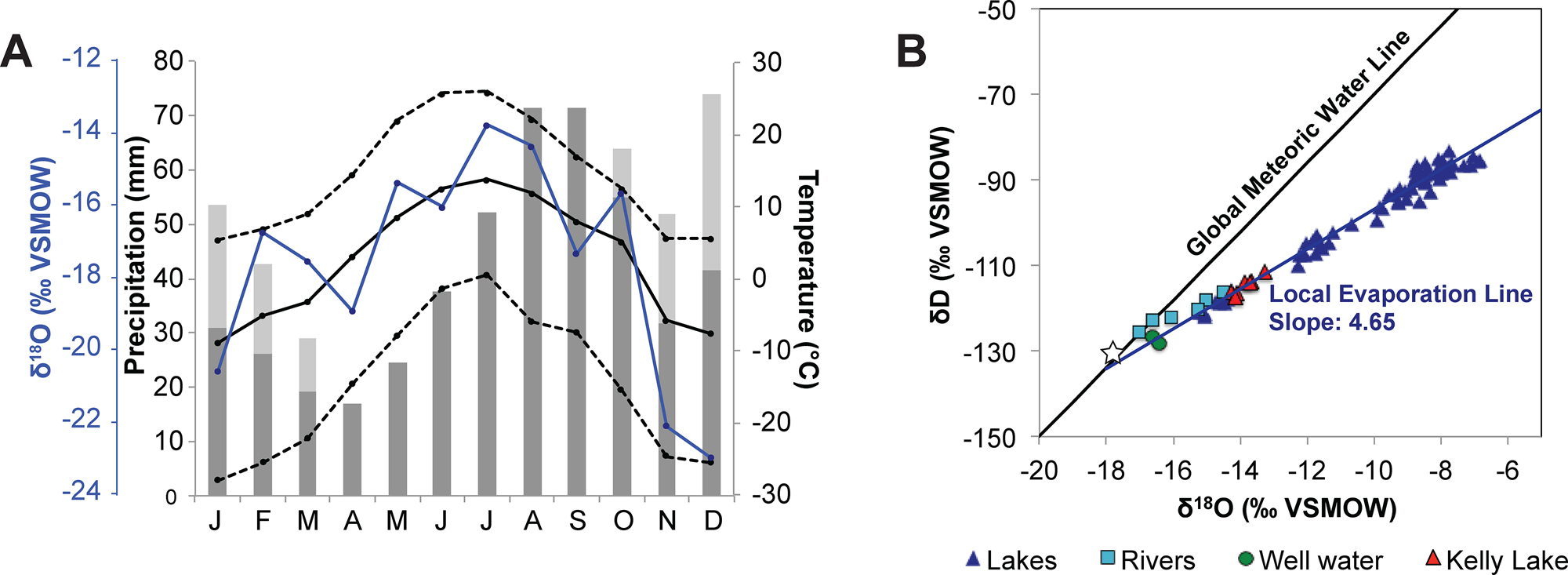
Figure 2. (A) Meteorological data from the Kenai Moose Pens SNOTEL station in Soldotna (https://www.nrcs.usda.gov/wps/portal/wcc/home/), showing the average (solid line), high (upper dashed line), and low (lower dashed line) temperatures alongside average monthly precipitation (dark-gray bars) and average monthly snow-water equivalent (SWE; light-gray bars) for 1995–2019 CE. The blue line shows monthly precipitation oxygen isotope values (δP) recorded at Tideview Station in Anchorage for 2005–2018 CE (Bailey et al., Reference Bailey, Klein and Welker2019). (B) Water isotope data for lakes, rivers, and groundwater in the Kenai lowlands collected between 2017 and 2018 CE (Broadman et al., Reference Broadman, Kaufman, Henderson, Berg, Anderson, Leng, Stahnke and Muñoz2020), shown with Local Evaporation Line (dark blue) plotted for all lake water samples, and the Global Meteoric Water Line (black). The annual average δP, weighted by monthly precipitation amount (shown in A), is indicated by the white star.
The Kenai Peninsula lowlands are dotted with kettle lakes that formed as the Cordilleran Ice Sheet retreated to both the Kenai Mountains and the Alaska Range following the Naptowne glaciation (Fig. 1C). The retreat of ice from its maximum extent was punctuated by several distinct stades throughout the Late Pleistocene, described by Reger et al. (Reference Reger, Sturmann, Berg and Burns2007). During the penultimate stade in this progression, the Skilak stade, lakes in the eastern Kenai lowlands located close to the mountains remained heavily influenced or occupied by glaciers. At this time, Kelly Lake (60.516°, −150.380°; 94 m asl) was deglaciated, but received meltwater from the glacier that occupied the Hidden Lake trough (60.485°, −150.267°; 86 m asl), ~4 km to the southeast (Fig. 1C). One event associated with termination of the Skilak stade is retreat of the Hidden Lake lobe, which halted the deposition of rock flour and meltwater in Hidden Lake's catchment. As such, the minimum limiting age for the Skilak stade termination is based on the transition between glaciolacustrine sediment and gyttja in a sediment core previously analyzed from Hidden Lake (Ager, Reference Ager and Wright1983), which is dated at ca. 16.6 ± 0.3 ka cal BP. This date is based on a bulk sediment sample originally analyzed using liquid scintillation (Ager, Reference Ager and Wright1983), and has been recalibrated in this study after Reimer et al. (Reference Reimer, Austin, Bard, Bayliss, Blackwell, Bronk Ramsey and Butzin2020).
The final stade of the Naptowne glaciation, the Elmendorf stade, has been associated with a Late Pleistocene readvance during the Younger Dryas (Reger et al., Reference Reger, Sturmann, Berg and Burns2007) and the subsequent retreat of glaciers from the Kenai lowlands by ca. 11 cal ka BP (Fig. 1C). Evidence for this latest stade in the Kenai lowlands is less robust than in the Matanuska and Knik valleys and in the Chugach Mountains, north of the Kenai Peninsula (Reger and Updike, Reference Reger, Updike, Péwé and Reger1983; Reger et al., Reference Reger, Combellick, Brigham-Grette, Combellick and Tannian1995, Reference Reger, Lowell and Evenson2011; Wiedmer et al., Reference Wiedmer, Montgomery, Gillespie and Greenberg2010; Kopczynski et al., Reference Kopczynski, Kelley, Lowell, Evenson and Applegate2017; Valentino et al., Reference Valentino, Owen, Spotila, Cesta and Caffee2021).
Today, glaciers terminate ~25 km southeast of Hidden Lake, and both Kelly and Hidden lakes are surrounded by boreal forest (Fig. 1C). Neither lake has a perennial surface inflow, although each lake has a minor surface outflow. Upwelling subaqueous springs are visible at the shallow eastern edge of Kelly Lake; the groundwater discharge likely comes from one of the two aquifers (surficial and deep) underlying the Kenai lowlands (Eilers et al., Reference Eilers, Landers, Newell, Mitch, Morrison and Ford1992).
METHODS
Sediment core recovery and sedimentological analyses
Sediment cores were collected from the depocenters of Hidden Lake (60.47226°, −150.21169°; 40 m water depth; Fig. 1E) and Kelly Lake (60.518770°, −150.39025°; 13 m water depth; Fig. 1D), from a raft in 2014 and 2018, respectively. The Hidden Lake core HD14-2 (252 cm long) and the uppermost 561 cm of the Kelly Lake sediment sequence (KLY18-2A) were collected using a percussion coring system. The stratigraphically lowest sections of the Kelly Lake sediment sequence (KLY18-2B) were collected using a 5-cm-diameter Livingstone piston corer, yielding a total length of 825 cm for composite core KLY18-2. An additional core collected from Kelly Lake, KLY18-4, also has been analyzed by Wrobleski (Reference Wrobleski2021).
Following recovery, cores were transported to the National Lacustrine Core Facility (LacCore) at the University of Minnesota, Minneapolis, where they were split, described, and analyzed for magnetic susceptibility (MS) and reflectance spectroscopy (between 400 and 700 nm) with a Geotek MSCL-XYZ automated core logger at 5 mm spacing. MS was analyzed using a Bartington MS2E surface probe, and reflectance was analyzed using a Konica Minolta spectrometer. The relative absorption-band depth (RABD) between 660 and 670 nm (RABD660;670) was calculated using Equation (1):

where R590 is reflectance at 590 nm, R730 is reflectance at 730 nm, and Rmin(660;670) is the minimum reflectance at either 660 or 670 nm (Rein and Sirocko, Reference Rein and Sirocko2002). RABD660;670 yields an estimate of sedimentary chlorin abundance, the diagenetic product of chlorophyll, which has absorption maxima between 660 and 690 nm (Wolfe et al., Reference Wolfe, Vinebrooke, Michelutti, Rivard and Das2006). RABD660;670 values are proportional to actual chlorin content, with typical values for lake sediments between ~1 and 2 (Butz et al., Reference Butz, Grosjean, Fischer, Wunderle, Tylmann and Rein2015).
Additional sedimentological analyses completed for these cores include bulk organic-matter content (OM), grain size distribution, and biogenic silica content (BSi). OM was measured using loss on ignition for every 3–4 cm of HD14-2, and for every 1–2 cm for KLY18-2. Each 1 cm3 (HD14-2) or 2.5 cm3 (KLY18-2) sample was weighed and dried overnight in an oven, then re-weighed and burned at 550°C for 2 hours, and finally weighed again to estimate OM content (Dean, Reference Dean1974). Grain size analysis was performed on 83 samples at ~5 cm increments throughout HD14-2. Samples weighing 0.2–0.6 g were treated with 30% H2O2 to remove organic matter and 10% Na2CO3 to remove biogenic silica, and were subsequently deflocculated in 5% Na6[(PO3)6]. Grain size was measured by laser diffraction using a LS-230 Beckman-Coulter analyzer, with 30 seconds of ultrasonic dispersion completed before each run. Finally, BSi was determined for samples from KLY18-2 using wet-alkaline extraction (10% Na2CO3), molybdate-blue reduction, and spectrophotometry (Mortlock and Froelich, Reference Mortlock and Froelich1989). Sampling resolution was every 1 cm for the upper 30 cm, and every 8–9 cm downcore (n = 130). A duplicate was analyzed for every 4 or 5 samples (n = 30) to determine the reproducibility of the procedure. Duplicates were processed in separate batches, and samples in each batch were selected randomly from all sample depths. Analytical reproducibility of the procedure, as indicated by differences between duplicate samples, averages 1.5 ± 1.0% (1σ).
Geochronology and proxy time-series correlations
Core chronologies were established using 10 (HD14-2) and 13 (KLY18-2) AMS 14C dates on plant and insect macrofossils (Table 1). For KLY18-2, aquatic plants were avoided due to the presence of a hard water effect. Sediment samples 1 cm thick were sieved at 150 μm, and macrofossils were picked, dried in an oven at 50°C, and identified under a Zeiss light microscope. Macrofossils were prepared and converted to graphite at Northern Arizona University, and 14C content was measured at the Keck-Carbon Cycle AMS facility at UC Irvine. Radiocarbon dates were incorporated into an age model for each sediment sequence using the R package Bacon (v2.5; Blaauw and Christen, Reference Blaauw and Christen2011), which calibrates 14C years to calendar years using IntCal20 (Reimer et al., Reference Reimer, Austin, Bard, Bayliss, Blackwell, Bronk Ramsey and Butzin2020).
Table 1. Radiocarbon (14C) ages for Hidden Lake core HD14-2 and Kelly Lake core KLY18-2. Depths are given as the midpoint of 1-cm-thick samples below lake floor (blf). Calibrated age is the median of the calibrated age probability density function. Uncertainty is one half of the calibrated two-sigma (2σ) range.

*Denotes a sample excluded from the Bacon age models.
To supplement the 14C chronology for the Kelly Lake sediment sequence, 210Pb and 137Cs profiles were used to constrain the chronology for the last ca. 170 years of core KLY18-2 (Supplementary Fig. 1; Supplementary Table 1). 210Pb, 214Pb, and 137Cs γ-activities were measured on 20 oven-dried and powdered samples from the upper 50 cm of surface core KLY18-2C using a Canberra Broad Energy Germanium Detector (BEGe; model no. BE3830P-DET) housed at the Marine Science Center of Northeastern University, with a count time of 24 hours. The Constant Rate of Supply (CRS) model (Appleby, Reference Appleby, Last and Smol2001) was used to estimate ages and confidence intervals of the samples with excess 210Pb activities above equilibrium with 214Pb.
Because several of the proxy datasets presented in this study are indicators of past productivity (especially chlorin, organic matter [OM], and biogenic silica [BSi] abundances), we calculated the extent to which these time series are correlated. For time series from the same site (either Hidden Lake or Kelly Lake), data were first resampled to average over the intervals of the time series with lower temporal resolution using the software package Analyseries (Paillard et al., Reference Paillard, Labeyrie and Yiou1996), and a correction for autocorrelation was performed (Bretherton et al., Reference Bretherton, Widmann, Dymnikov, Wallace and Bladé1999). To determine relationships among time series between Hidden and Kelly lakes, the ensemble outputs from the Bacon age models were used to calculate age-uncertain correlations with the R package geoChronR (v.1.0.6; McKay et al., Reference McKay, Emile-Geay and Khinder2021). Proxy data were binned into 500-year intervals prior to correlation. Significance was estimated with an “isospectral” approach, where characteristics of the time series’ power spectra are incorporated into significance testing to assess the impact of autocorrelation and other biases (Ebisuzaki, Reference Ebisuzaki1997). To avoid the possibility of test multiplicity when correlating among many ensemble members, a 5% false discovery rate (FDR) correction was applied, which controls for spurious correlations that might arise as an artifact of repeated testing (Benjamini and Hochberg, Reference Benjamini and Hochberg1995; Ventura et al., Reference Ventura, Paciorek and Risbey2004).
Pollen and macrofossils
To correlate the pollen zones identified by Ager (Reference Ager and Wright1983) with our dataset from HD14-2, 11 samples from core HD14-2 were analyzed for pollen following standard protocols (Faegri and Iverson, Reference Faegri and Iversen1989). Using these newly acquired data, the stratigraphic positions of the Ager (Reference Ager and Wright1983) pollen zones were located in HD14-2 (Supplementary Table 2), and revised ages were assigned using the output of the Bacon age model. For this study, the pollen data were plotted as percent relative abundance using the R package Rioja (v.0.9-26; Juggins, Reference Juggins2017), and an incremental sum-of-squares cluster analysis (CONISS) was applied (Grimm, Reference Grimm1987) using the R package Vegan (v.2.5-7; Oksanen et al., Reference Oksanen, Kindt, Legendre, O'Hara, Henry and Stevens2007).
To complement the pollen data from Hidden Lake, 74 samples (1 cm thick; 10 cm increments) from KLY18-2 were analyzed for macrofossils. Limited material in the upper ~50 cm of KLY18-2 excluded these youngest sediments from macrofossil analyses. Samples were deflocculated in 5% Na6[(PO3)6] and then sieved at 125 and 250 μm to isolate macrofossil material. Identifiable terrestrial and aquatic plant macrofossils were counted, and then plotted as concentration per 10 cm3 using the R package Rioja (v.0.9-26; Juggins, Reference Juggins2017).
Diatom assemblages
Twenty 1-cm-thick samples from KLY18-2 were selected at 25–50 cm increments for diatom species analysis. Samples were treated with 30% H2O2 and 70% HNO3 to remove organic matter, then mounted on slides using Naphrax© medium. A Zeiss light microscope was used to count 300 valves per slide along transects at 1000X, and taxonomic classifications were made according to Foged (Reference Foged1971, Reference Foged1981), Krammer and Lange-Bertalot (1986–1991), McGlaughlin and Stone (1986), and Mann et al. (Reference Mann, McDonald, Mayer, Droop, Chepurnov, Loke, Ciobanu and Du Buf2004). Diatom species counts were converted to percent relative abundance and graphed using the R package Rioja (v.0.9-26; Juggins, Reference Juggins2017), and a CONISS analysis was applied to dominant taxa with a relative abundance >5% in at least one sample (Grimm, Reference Grimm1987) to determine zone designations, using the R package Vegan (v.2.5-7; Oksanen et al., Reference Oksanen, Kindt, Legendre, O'Hara, Henry and Stevens2007). A principal component analysis (PCA) (ter Braak and Prentice, Reference ter Braak and Prentice1988) was completed on the correlation matrix of untransformed percentage data for all dominant taxa. The proportion of planktonic diatoms was calculated as the sum of all planktonic taxa divided by the sum of all planktonic and benthic taxa (excluding facultatively planktonic diatoms) (Wang et al., Reference Wang, Mackay, Leng, Rioual, Panizzo, Lu, Gu, Chu, Han and Kendrick2013).
Diatom oxygen isotopes
Samples for diatom oxygen isotope (δ18Odiatom) analysis (1 cm thick) were taken from KLY18-2 every ~10 cm down core, and every 1 cm of the upper 25 cm (n = 107). Sampling avoided visible tephra layers, as well as basal sediments that contain few diatoms. Samples were purified using a series of chemical digestions, sieving, and heavy liquid separations (Morley et al., Reference Morley, Leng, Mackay, Sloane, Rioual and Battarbee2004). All samples were visually inspected for contamination under a Zeiss light microscope, and 27 samples were inspected further using a Zeiss Supra 40VP variable pressure field emission scanning electron microscope (SEM) (e.g., Supplementary Fig. 2) and energy dispersive X-ray spectroscopy (EDS). δ18Odiatom values were measured using the stepwise fluorination method (Leng and Sloane, Reference Leng and Sloane2008) in the stable isotope facility at the British Geological Survey, UK. δ18O values are reported as per mil (‰) deviations of the isotopic ratio (18O/16O) calculated on the VSMOW scale using a within-run laboratory standard calibrated against NBS-28. δ18O of the standard biogenic silica (BFC) run alongside the sample diatoms was set to + 28.9‰ (n = 26) ±0.1‰ (1σ) (Chapligin et al., Reference Chapligin, Leng, Webb, Alexandre, Dodd, Ijiri and Lücke2011). Analytical reproducibility of the sample material was <0.2‰ (1σ).
Hydrologic and isotope mass balance modeling
A simple hydrologic and isotope mass balance model was used (e.g., Gibson et al., Reference Gibson, Prepas and McEachern2002; Steinman et al., Reference Steinman, Rosenmeier, Abbott and Bain2010) to investigate steady state conditions at different intervals during the Holocene (e.g., Lacey and Jones, Reference Lacey and Jones2018), to test the sensitivity of the hydrologic budget to changes in multiple inputs during the past, and to calculate the contribution of groundwater to Kelly Lake. Hydrologic (eq. 2) and isotope (eq. 3) mass balance expressions typically used for lake systems at steady state are given as:


where Si and Gi are the surface and groundwater inflow rates, So and Go are the surface and groundwater outflow rates, P and E are the precipitation and evaporation rates, V is the volume of water in the lake (L), and T is time. In Equation (3), each term in Equation (2) is multiplied by the annually averaged isotope composition of each inflow (i) and outflow (o). Groundwater and surface water outflows (Go and So) are assumed to have the isotope composition of the lake water (δL).

For the modern period, most terms in Equation (4) can be represented using measured values (Tables 2, 3). For P, the mean annual precipitation rate from 1995–2018 measured at the Kenai Moose Pens SNOTEL station (Fig. 2A) was converted to the volume of on-lake precipitation. The monthly weighted average of annual precipitation oxygen isotopes measured from 2005–2018 at the Tideview Station in Anchorage was used for δP (Bailey et al., Reference Bailey, Klein and Welker2019; Fig. 2A). Measurements of δL at Kelly Lake and δGi from a well in Sterling, Alaska, were collected in 2017 and 2018 (Broadman et al., Reference Broadman, Kaufman, Henderson, Berg, Anderson, Leng, Stahnke and Muñoz2020; Fig. 2B), and were assumed to be representative of annual average values. The annual average evaporation rate recorded from 1917–2005 at the Western Regional Climate Center in Gateway, Alaska (~130 km northeast of Kelly Lake; https://wrcc.dri.edu/Climate/comp_table_show.php?stype=pan_evap_avg) is essentially identical (within 0.01 m/year) to that calculated using the Linacre (Reference Linacre1992) simplification of the Penman (Reference Penman1948) formula for open water evaporation at Kelly Lake, and this value was used for E.
Table 2. Climate and hydrologic variables used as inputs for the Kelly Lake hydrologic and isotope mass balance modeling for each time period discussed in the text. Values are for annual averages.
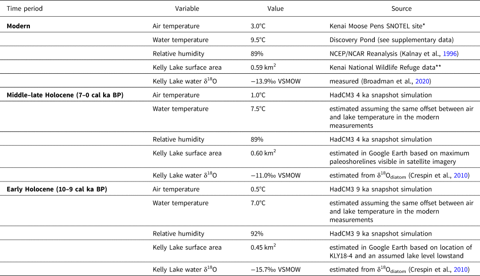
*Data for 1995–2018 from the National Water and Climate Center: https://www.nrcs.usda.gov/wps/portal/wcc/home/
**Data from the US Fish and Wildlife Service: https://www.fws.gov/refuge/Kenai/map.html
Table 3. Measurements and fluxes for hydrologic and isotopic inflows (precipitation, groundwater) and outflows (evaporation) used in the Kelly Lake modeling and sensitivity testing for each time period.

*Data for 1995–2018 from the National Water and Climate Center: https://www.wcc.nrcs.usda.gov/index.html
**Data from the Western Regional Climate Center: https://www.nrcs.usda.gov/wps/portal/wcc/home/
The isotope composition of evaporated water vapor (δE) was estimated using the Craig and Gordon (Reference Craig, Gordon and Tongiogi1965) evaporation model:

where δL is the isotope composition of the lake water. In Equation (5), α* is the reciprocal of the equilibrium isotope fractionation factor (α) estimated for δ18O in Equation (6) using the equation of Horita and Wesolowski (Reference Horita and Wesolowski1994), where TW is the temperature of the lake surface water (in K):

The normalized relative humidity (h) used in Equation (5) can be estimated using Equation (7) as the quotient of the saturation vapor pressure of the overlying air (es-a) and the saturation vapor pressure at the surface water temperature (es-w) (e.g., Steinman et al., Reference Steinman, Rosenmeier, Abbott and Bain2010). Both of these can be estimated with Equation (8) using annual average air temperature and surface lake water temperature, respectively. Annual average surface relative humidity (RH) for 1995–2018 was taken from the Kelly Lake grid cell of the NCEP/NCAR Reanalysis (Kalnay et al., Reference Kalnay, Manamitsu, Kistler, Collins, Deaven, Gandin and Iredell1996).


In lieu of year-round measurements of surface water temperature at Kelly Lake, we used the annual average surface water temperature measured from 2005–2007 at nearby Discovery Pond (~40 km to the northwest) in Equation (8) (Table 2; Supplementary Data).
The isotope composition of atmospheric moisture (δA) used in Equation (5) is assumed to be in equilibrium with precipitation in Equation (9). The equilibrium isotope separation factor (ɛ*) is the difference between the isotope composition of precipitation and atmospheric moisture (Gibson et al., Reference Gibson, Prepas and McEachern2002; eq. 10), known to be a function of temperature (Gonfiantini, Reference Gonfiantini, Fritz and Fontes1986; eq. 6). The total isotope separation factor (ɛ; eq. 11) also comprises a kinetic component (ɛK; Gibson et al., Reference Gibson, Prepas and McEachern2002), which can be constrained for oxygen isotope fractionation (Gonfiantini, Reference Gonfiantini, Fritz and Fontes1986; eq. 12).


To use the Krabbenhoft et al. (Reference Krabbenhoft, Bowser, Anderson and Valley1990) model (eq. 4) to investigate past environmental conditions, variables must be inferred from climate model output or derived empirically. Deriving δE (eq. 5) requires estimates for RH, air temperature, and water temperature; for these, and for estimates of P and E, we used the original (not downscaled) output of “snapshot” simulations performed using the coupled ocean-atmosphere circulation model HadCM3 (Singarayer and Valdes, Reference Singarayer and Valdes2010) (Tables 2, 3). Estimates were taken from snapshots for 9 ka (to investigate the Early Holocene) and 4 ka (to investigate the Middle to Late Holocene). Although approximate, these simulations provide appropriate past annual average baseline conditions that we used to assess hydrologic and isotope mass balance at Kelly Lake.
As might be expected, the mean values of variables from the climate simulation are somewhat different from the observed values for these variables near Kelly Lake (Supplementary Table 3). Simulated surface air temperature is ~2–3°C lower than observed at Kenai airport (air temperature; https://www.ncdc.noaa.gov/cdo-web/datasets), simulated precipitation is 0.05 m/year higher than observed at the Kenai Moose Pens SNOTEL station, and simulated evaporation is 0.09 m/year lower than observed at the Western Regional Climate Center station in Gateway. This might be because of relatively low-resolution parameterization and lack of downscaling, or because the simulations are not fully transient (Singarayer and Valdes, Reference Singarayer and Valdes2010), both of which might result in simulated conditions that fail to fully account for feedbacks of slow-responding components of the climate system. As such, for variables inferred from the HadCM3 simulations, we performed a bias adjustment by calculating the difference between observed recent climate data and the 0 ka HadCM3 simulation, and then applying this difference to the 9 ka and 4 ka values for each variable (Supplementary Table 3). This bias adjustment allows for a direct comparison between modern conditions at Kelly Lake, and the simulated difference between modern and past conditions. The offset between the surface air temperature and the surface water temperature was assumed to be equal to that recorded in the modern period at Discovery Pond (Table 2).
Estimates for P and E in Equation (4) require values both for precipitation and evaporation rates, and for lake surface area (Table 2). Uncertainties in the precipitation and evaporation rates were incorporated into sensitivity testing by modeling scenarios where P and E might be up to 25% higher or lower compared to the HadCM3-inferred values. Current and estimated maximum lake surface areas were measured from Google Earth satellite imagery taken in 2019. An estimate for the minimum lake surface area was based on bathymetry and evidence for continuous postglacial sedimentation at the shallow water core site, KLY18-4 (Wrobleski, Reference Wrobleski2021; Supplementary Fig. 3).
The approximate isotope composition of past lake water (δL) in Equation (4) was inferred from sedimentary δ18Odiatom values (Table 2). These estimates capture the magnitude of past changes, but the absolute value of past δL depends on the oxygen isotope fractionation factor between sedimentary diatom silica and lake water. There is consensus that this temperature-dependent equilibrium fractionation factor between cultured or living diatoms and lake water is approximately −0.2‰/°C (Brandriss et al., Reference Brandriss, O'Neil, Edlund and Stoermer1998; Moschen et al., Reference Moschen, Lücke and Schleser2005; Crespin et al., Reference Crespin, Sylvestre, Alexandre, Sonzogni, Pailles and Perga2010; Dodd and Sharp, Reference Dodd and Sharp2010). However, calibration studies based on sedimentary diatoms have yielded fractionation factors as large as −0.49‰/°C (Juillet-Leclerc and Labeyrie, Reference Juillet-Leclerc and Labeyrie1987; Shemesh et al., Reference Shemesh, Charles and Fairbanks1992), and a growing body of evidence suggests rapid geochemical alteration may overprint the δ18O of diatom silica in the decades following deposition (Dodd et al., Reference Dodd, Wiedenheft and Schwartz2017; Menicucci et al., Reference Menicucci, Spero, Matthews and Parikh2017; Tyler et al., Reference Tyler, Sloane, Rickaby, Cox and Leng2017). There is no clear solution to account for this possible diagenetic alteration in paleoenvironmental reconstructions, but we acknowledge that it adds uncertainty to reconstructing δL based on sedimentary δ18Odiatom. However, the lack of a consistent trend over the past several centuries among the δ18Odiatom values in datasets from this region (e.g., Schiff et al., Reference Schiff, Kaufman, Wolfe, Dodd and Sharp2009; Bailey et al., Reference Bailey, Kaufman, Sloane, Hubbard, Henderson, Leng, Meyer and Welker2018; Broadman et al., Reference Broadman, Kaufman, Henderson, Berg, Anderson, Leng, Stahnke and Muñoz2020; this study) indicates that these diagenetic effects are unlikely to systematically affect paleoenvironmental interpretations based on sedimentary δ18Odiatom data.
Inferring δL from δ18Odiatom also requires consideration of diatom ecology and diatom oxygen isotope systematics. Oxygen isotope fractionation between diatom silica and lake water occurs not only while a diatom is alive, but also while it sinks through the water column and settles on the lake floor (Dodd and Sharp, Reference Dodd and Sharp2010; Dodd et al., Reference Dodd, Sharp, Fawcett, Brearley and McCubbin2012; Tyler et al., Reference Tyler, Sloane, Rickaby, Cox and Leng2017). Therefore, while a diatom might dwell in the water column or near the water's surface during its life, the isotope signature recorded in a sedimentary diatom frustule will be at least partially overwritten by fractionation occurring at the lake floor. As such, we used 4°C as an estimate of average annual bottom water temperature (Vallentyne, Reference Vallentyne1957) to examine the modern (2018) relationship between δL and δ18Odiatom in Kelly Lake surface sediments. We found that the fractionation factor of −1.16‰/°C calculated by Crespin et al. (Reference Crespin, Sylvestre, Alexandre, Sonzogni, Pailles and Perga2010) (eq. 13), which can be rearranged to calculate δL (eq. 14), best captures the relationship between temperature, δL, and δ18Odiatom at our site:


where T is in °C, and δ18O values are in ‰ VSMOW. For the modern calculation, the average of the three youngest Kelly Lake δ18Odiatom values was used (from the uppermost 3 cm; mean = +24.6‰) to account for the probable effects of bioturbation and sediment mixing on the unconsolidated uppermost lake sediments. Using this modern δ18Odiatom value and a temperature of 4°C, Equation (14) yields a δL value of −14.0‰, which is analytically indistinguishable from the measured average value of −13.9‰ for Kelly Lake water (Broadman et al., Reference Broadman, Kaufman, Henderson, Berg, Anderson, Leng, Stahnke and Muñoz2020; Fig. 2B).
Equation (4) also requires an estimate of δP, which is difficult to constrain with certainty for past periods, because few Holocene isotope-enabled model simulations exist, especially for the Early Holocene. Therefore, we tested scenarios where δP values are much higher compared with today (similar to summer precipitation; −14.7‰), much lower compared with today (similar to winter precipitation −20.7‰), and similar to the modern annual average (−17.7‰). These values are in line with the magnitude of δP fluctuations inferred from other nearby paleo oxygen isotope datasets (Jones et al., Reference Jones, Wooller and Peteet2014, Reference Jones, Anderson, Keller, Nash, Littell, Wooller and Jolley2019; Bailey et al., Reference Bailey, Kaufman, Sloane, Hubbard, Henderson, Leng, Meyer and Welker2018; Broadman et al., Reference Broadman, Kaufman, Henderson, Berg, Anderson, Leng, Stahnke and Muñoz2020) (Table 3). ΔGi is heavily influenced by δP, and therefore was assumed to be within 1.5‰ of δP in all scenarios (Table 3). These scenarios were used to determine the components of the lake's hydrologic budget that most likely caused inferred changes in δL, as reflected by sedimentary δ18Odiatom, during different intervals of the Holocene. Tests were performed for three time periods: (1) modern, (2) Early Holocene (using inputs from the 9 ka HadCM3 snapshot), and (3) Middle to Late Holocene (using inputs from the 4 ka HadCM3 snapshot).
When determining model inputs for δP and δGi in Equation (4), necessary reasonable assumptions were made to ensure logical results (i.e., a positive value for Gi). To use this mass balance model (eq. 4), the values for δP, δE, and δGi must all be lower than δL (Krabbenhoft et al., Reference Krabbenhoft, Bowser, Anderson and Valley1990). δE is empirically derived (described above), and is necessarily lower than δL (Craig and Gordon, Reference Craig, Gordon and Tongiogi1965). It is also reasonable to assume that δL is always higher than the annual averages of both δP and δGi (e.g., Fig. 2B) due to the effects of evaporative isotope enrichment, a phenomenon that does not significantly affect either δP or δGi. The assumption that δL is always higher than δGi is critical for this simplified model, because Gi asymptotes as δL approaches δGi. Consequently, we do not simulate conditions where δL − δGi < 0.5, and we did not model scenarios where δP or δGi values violated this or any other aforementioned assumptions of the mass balance model equation.
RESULTS
Sediment properties
Basal sediments of the Hidden Lake core HD14-2 are composed of interbedded, gray, inorganic clay and silt, assumed to have been deposited while glaciers occupied the catchment. Postglacial sediments (above 228.2 cm) from HD14-2 are composed primarily of gyttja, which is interbedded with gray silt and clay for the stratigraphically lowest ~60 cm (Fig. 3). The sediment sequence contains 15 visible tephra beds (≥1 mm thick) that correspond to peaks in MS (Fig. 3; Supplementary Table 4). Above 228.2 cm, organic matter content (as measured by LOI) fluctuates between 1.5 and 21.0% (mean = 10.0%), and inferred chlorin content (as measured by RABD660;670) fluctuates between 1.00 and 1.18 (mean = 1.07). Median grain size (d50) ranges from 5–24 μm, and the coarsest grain-size fraction (d90) ranges from 32–175 μm (Fig. 3).
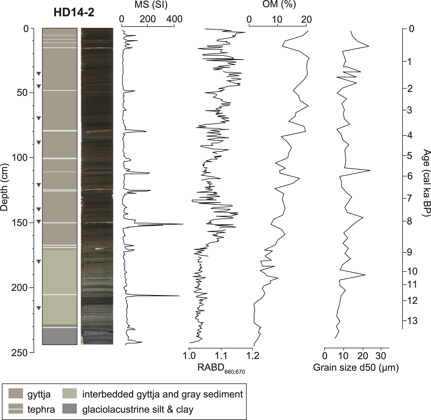
Figure 3. Stratigraphy of Hidden Lake core HD14-2 with magnetic susceptibility (MS), inferred chlorin content (RABD660;670), organic matter (OM), and the 50th percentile of clastic grain size (d50). Age scale is based on the age model shown in Figure 5. Gray triangles show calibrated 14C ages listed in Table 1.
Kelly Lake sediments are predominantly composed of gyttja, with 27 visible tephra beds (≥1 mm thick) that correspond to peaks in MS (Fig. 4; Supplementary Table 4). The basal ~60 cm of KLY18-2 is carbonate-rich mud interbedded with organic-rich clastic layers (Fig. 4). OM content ranges from 7–92% (mean = 33%), and inferred chlorin content ranges from 0.87–2.55 (mean = 1.33). BSi ranges from 1.0–34.6% (mean = 24.6%), with the lowest values in the basal carbonate mud. Correlations among indicators of past productivity (chlorin, organic matter, and BSi abundances) are shown for datasets within the same lake (Supplementary Fig. 4), and for datasets between different lakes (Supplementary Fig. 5) as histograms for the age-uncertain correlations.
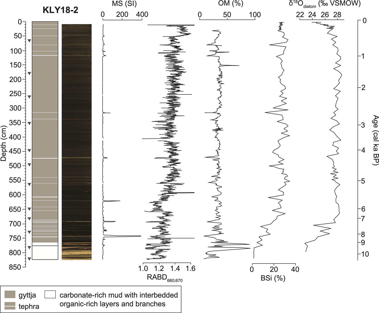
Figure 4. Stratigraphy of Kelly Lake core KLY18-2 with magnetic susceptibility (MS), inferred chlorin content (RABD660;670), organic matter (OM), biogenic silica (BSi), and diatom oxygen isotopes (δ18Odiatom). Age scale is based on the age model shown in Figure 5. Gray triangles show calibrated 14C ages listed in Table 1.
Geochronology
The oldest 14C age from Hidden Lake core HD14-2 is 12,618 ± 97 cal yr BP at 216.7 cm, 11.5 cm above the transition from glaciolacustrine mud to organic-rich sediment (Table 1). The extrapolated age for this transition is 13,089 ± 671 cal yr BP (Fig. 5). The average 95% confidence interval of the Bacon age model, evaluated every 1 cm back to 13,824 ± 955 cal yr BP, is ± 756 years (min = 4; max = 1909 years). One 14C age was excluded from the age model (UCIAMS 147382) because it deviates from the roughly linear downcore trend from the other 14C ages. Average sediment accumulation rate for the postglacial sediment (above 228.2 cm) is 0.17 mm/year. The Hayes tephra, identified at 79.2 cm in Hidden Lake and 473.0 cm in Kelly Lake based on preliminary geochemical analyses (B. Jensen, personal communication, 2020), is dated at 3837 ± 302 cal yr BP and 4234 ± 180 cal yr BP, respectively (Supplementary Table 4). These age ranges are consistent with previous estimates for the multiple deposits associated with Hayes eruptions at this time (Wallace et al., Reference Wallace, Coombs, Hayden and Waythomas2014; Davies et al., Reference Davies, Jensen, Froese and Wallace2016).
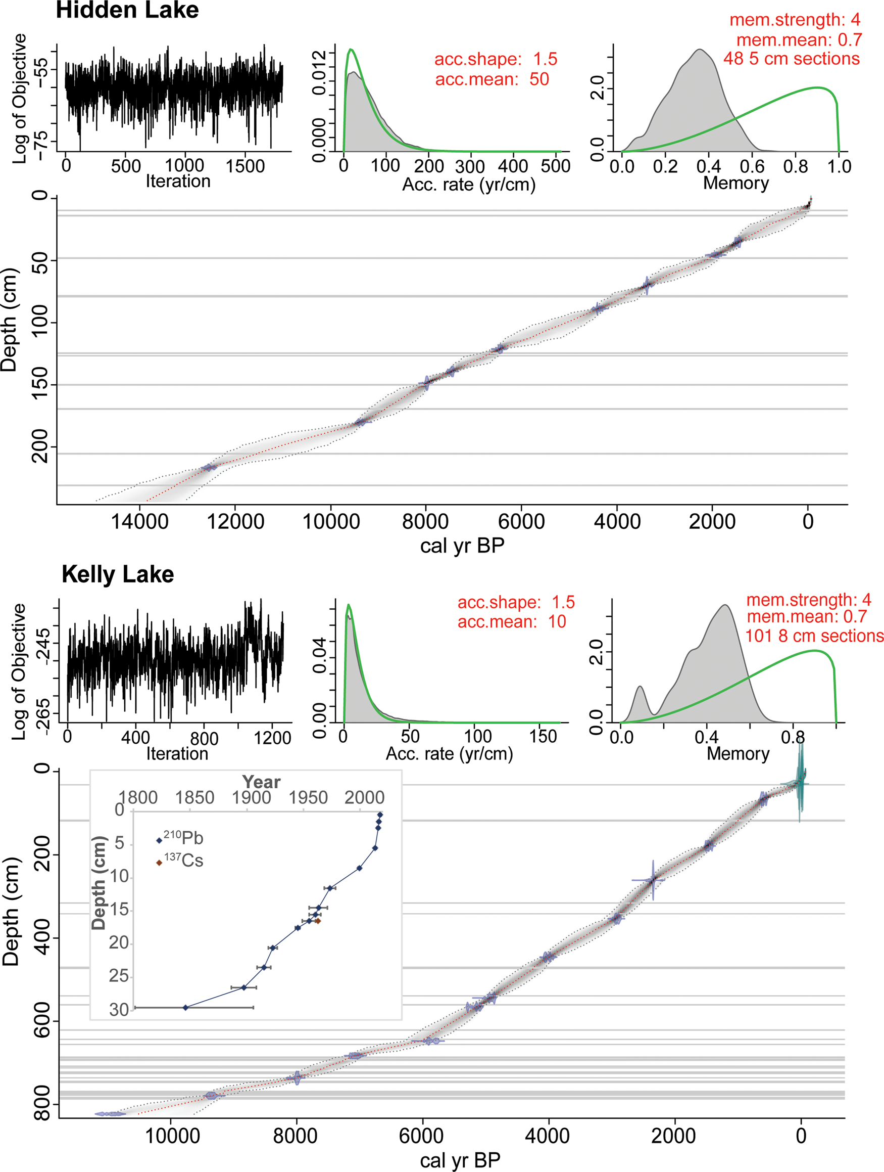
Figure 5. Age-depth models for Hidden Lake core HD14-2 and Kelly Lake core KLY18-2, created using Bacon (v2.2; Blaauw and Christen, Reference Blaauw and Christen2011). Gray horizontal lines mark visible tephra deposits (as well as large branches in Kelly Lake) that are assumed to have been deposited instantaneously. The depths and basal ages of the tephra layers are in Supplementary Table 3. Inset shows the 210Pb and 137Cs profile of the near-surface sediments from Kelly Lake (data in Supplementary Fig. 2 and Supplementary Table 1).
The oldest 14C age from Kelly Lake core KLY18-2 is 10,940 ± 200 cal yr BP at 823 cm, which is at the base of the core. The average 95% confidence interval for the age model is ± 200 years (min = 1; max = 683 years). One 14C age from an aquatic plant stem (UCIAMS 208325) was excluded from the age model; the sample was analyzed prior to realizing the influence of the hard water effect (Philippsen, Reference Philippsen2013) on aquatic macrofossil samples from Kelly Lake. Sedimentation rate increases from ~0.4 mm/year to 1.0 mm/year, starting at ca. 6500 cal yr BP. The 210Pb activities exhibit a gradual decline over the upper 36 cm of core KLY18-2C towards an equilibrium of ~11.7 Bq/kg (Supplementary Fig. 1; Supplementary Table 1). The peak in 137Cs activity at 16.5 cm (Supplementary Fig. 1) was used as a reference level to constrain the 210Pb model (Appleby, Reference Appleby, Last and Smol2001).
Pollen
Using the pollen data from core HD14-2, we detected the stratigraphic positions of the pollen zone transitions identified by Ager (Reference Ager and Wright1983) (Supplementary Table 2) in the new sediment sequence and determined ages for these zones according to the Bacon age model (Fig. 6). Ager (Reference Ager and Wright1983) described five major pollen zones, listed below, with the original stratigraphic depths from Ager (Reference Ager and Wright1983) and our updated ages from HD14-2.

Figure 6. Relative abundance of dominant pollen types in Hidden Lake from Ager (Reference Ager and Wright1983), shown alongside new ages and approximate depths associated with the pollen data from core HD14-2 and the corresponding age model shown in Figure 5. Pollen types include conifers (dark green), deciduous trees (pale green), and shrubs and grasses (orange). Dashed lines show the originally identified vegetation zones (Ager, Reference Ager and Wright1983). CONISS-designated clusters are shown on the right. Analyzed and plotted using the R packages Rioja (v.0.9-26; Juggins, Reference Juggins2017) and Vegan (v.2.5-7; Oksanen et al., Reference Oksanen, Kindt, Legendre, O'Hara, Henry and Stevens2007).
Zone 1 (13.6–12.9 cal ka BP; 290–260 cm)
Zone 1, the “herb zone,” is characterized by a high relative abundance of Cyperaceae (sedge) pollen, as well as the presence of Poaceae (grasses) and Artemisia (mugwort, wormwood, sagebrush). Salix (willow) is present (~5–10% abundance), probably as a dwarf shrub (Ager, Reference Ager and Wright1983), as has been inferred for other sites in the Kenai lowlands (e.g., Anderson et al., Reference Anderson, Hallett, Berg, Jass, Toney, de Fontaine and DeVolder2006, Reference Anderson, Berg, Williams and Clark2019). Arboreal taxa are absent from this zone, suggesting a landscape dominated by herbaceous taxa.
Zone 2 (12.9–11.0 cal ka BP; 260–205 cm)
Zone 2, the “Betula zone,” is dominated by Betula (birch) pollen, interpreted by Ager (Reference Ager and Wright1983) to reflect a dwarf-birch shrub tundra. Salix and tundra taxa that are dominant in Zone 1 remain present.
Zone 3 (11.0–9.3 cal ka BP; 205–190 cm)
Zone 3, the “Populus and Salix zone,” is characterized by a decrease in the abundance of Betula and an increase in the abundance of Populus (cottonwood) and Salix pollen. Herbaceous taxa remain present. The first occurrence of Alnus (alder) is recorded this zone. These changes indicate a transition from dwarf-birch tundra to a mixture of scrub forest and shrub tundra (Ager, Reference Ager and Wright1983).
Zone 4 (9.3–8.6 cal ka BP; 190–170 cm)
Zone 4, the “Alnus zone,” is characterized by high Alnus pollen values and declines in the abundance of all other taxa, indicating the development of an alder woodland. Picea (spruce) makes its first appearance at the end of this zone.
Zone 5 (8.6 cal ka BP–present; 170–0 cm)
Zone 5, the “Picea, Alnus, and Betula zone,” is characterized by the increased relative abundance of Picea pollen and the continued presence of Betula and Alnus. Most other previously documented taxa remain present, but in low abundances (<5%). These pollen data indicate the transition from an alder woodland to a spruce, birch, and alder forest (Ager, Reference Ager and Wright1983). Tsuga mertensiana (mountain hemlock) pollen appears in the upper 80 cm, indicating arrival of the species in the region at this point. Although we do not have a clear tie point to relate the arrival of T. mertensiana to our new age model, if we assume a linear sediment accumulation rate between the sediment surface and the first dated pollen zone transition reported by Ager (Reference Ager and Wright1983), this event can be crudely estimated at ca. 4 cal ka BP, which is ca. 1000–2000 years earlier than suggested for the Kenai Peninsula by Anderson et al. (Reference Anderson, Kaufman, Berg, Schiff and Daigle2017).
Macrofossils
The Kelly Lake terrestrial macrofossil data reveal shifts in the vegetation communities of the catchment from ca. 10,300–500 cal yr BP (Fig. 7), which closely reflects the vegetation transitions indicated by the Hidden Lake pollen data. Betula bracts and/or fruits are present throughout the nearly 11,000-year sediment sequence, whereas Alnus bracts and fruits and Picea needles first appear at ca. 8155 cal yr BP (Fig. 7). Bryophytes (mosses) are present continually throughout the sediment sequence. In addition, bryozoan statocysts (zooids) are present intermittently, but are concentrated in the sediments prior to ca. 8000 cal yr BP and again following ca. 5000 cal yr BP. Chara oospores, which are most prevalent prior to ca. 5500 cal yr BP, persist until ~ca. 900 cal yr BP.
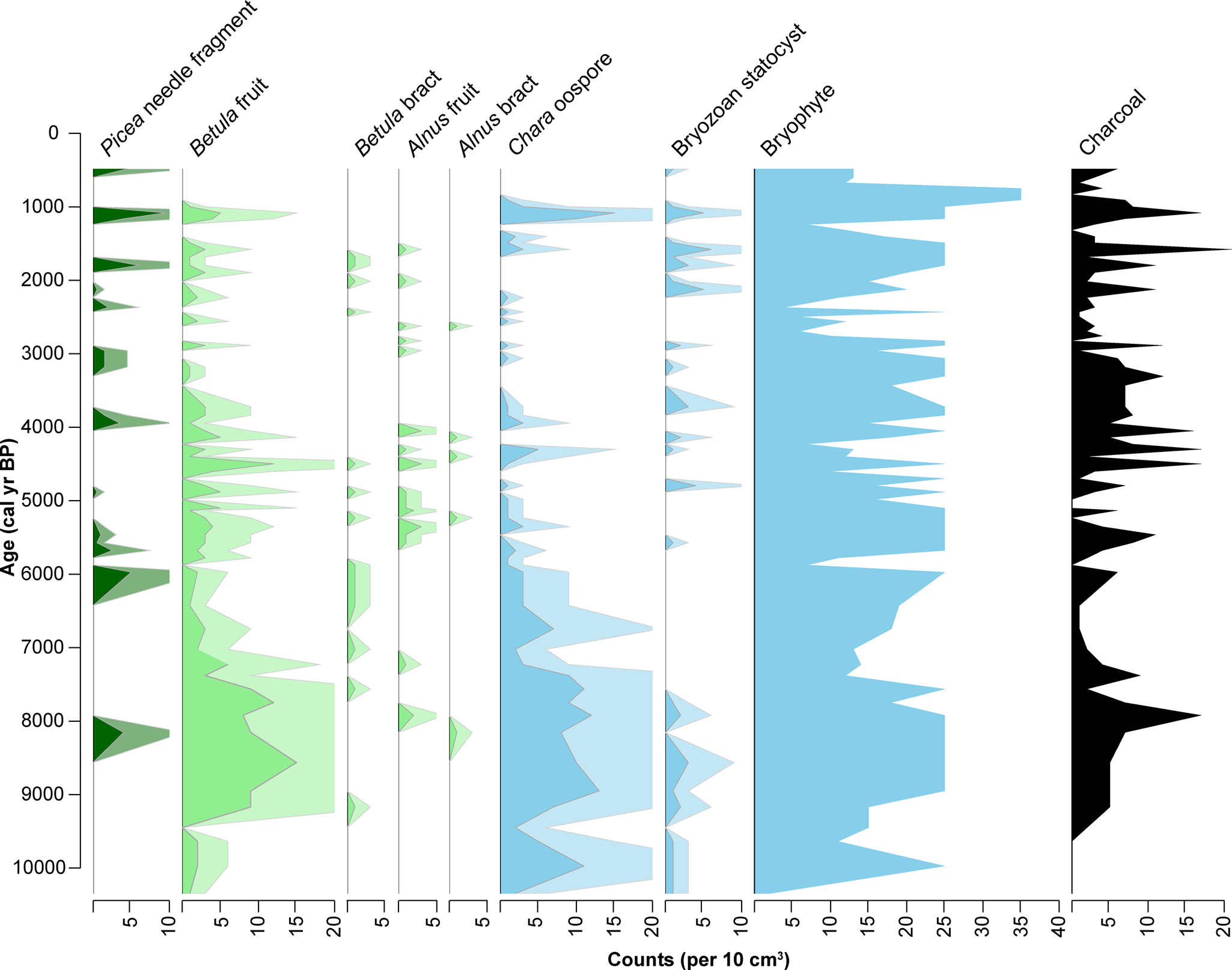
Figure 7. Concentration of terrestrial (green), aquatic (blue), and charcoal macrofossils identified in Kelly Lake core KLY18-2. Analyzed and plotted using the R package Rioja (v.0.9-26; Juggins, Reference Juggins2017). Pale shading is a 3x exaggeration of the actual concentration.
Diatom assemblages
The diatom assemblages from Kelly Lake are diverse, comprising 148 taxa in total, from which 12 species were classified as dominant (those with a relative abundance of >5% in at least one sample) (Fig. 8). Diatoms were too few to count in the basal carbonate-rich mud, and the diatom assemblage data therefore extend back to ca. 9.2 cal ka BP. Dominant species were grouped into one of three habitat types, as specified by Spaulding et al. (Reference Spaulding, Bishop, Edlund, Lee and Potapova2020): (1) planktonic diatoms, which are non-motile and occupy the water column; (2) facultatively planktonic diatoms, which may be motile, often dwelling in the lake's benthos, but can live in the water column when it is ecologically advantageous; and (3) benthic diatoms, which can be motile, or live attached to substrates on the lake floor or in shallow sediments. Dominant genera at Kelly Lake include planktonic (Aulacoseira, Discostella), facultatively planktonic (Staurosira, Staurosirella), and benthic (Pseudostaurosira, Staurosirella) diatoms. Based on the CONISS dendrogram, changes in the relative abundances of these taxa were divided into two main zones (Fig. 8).
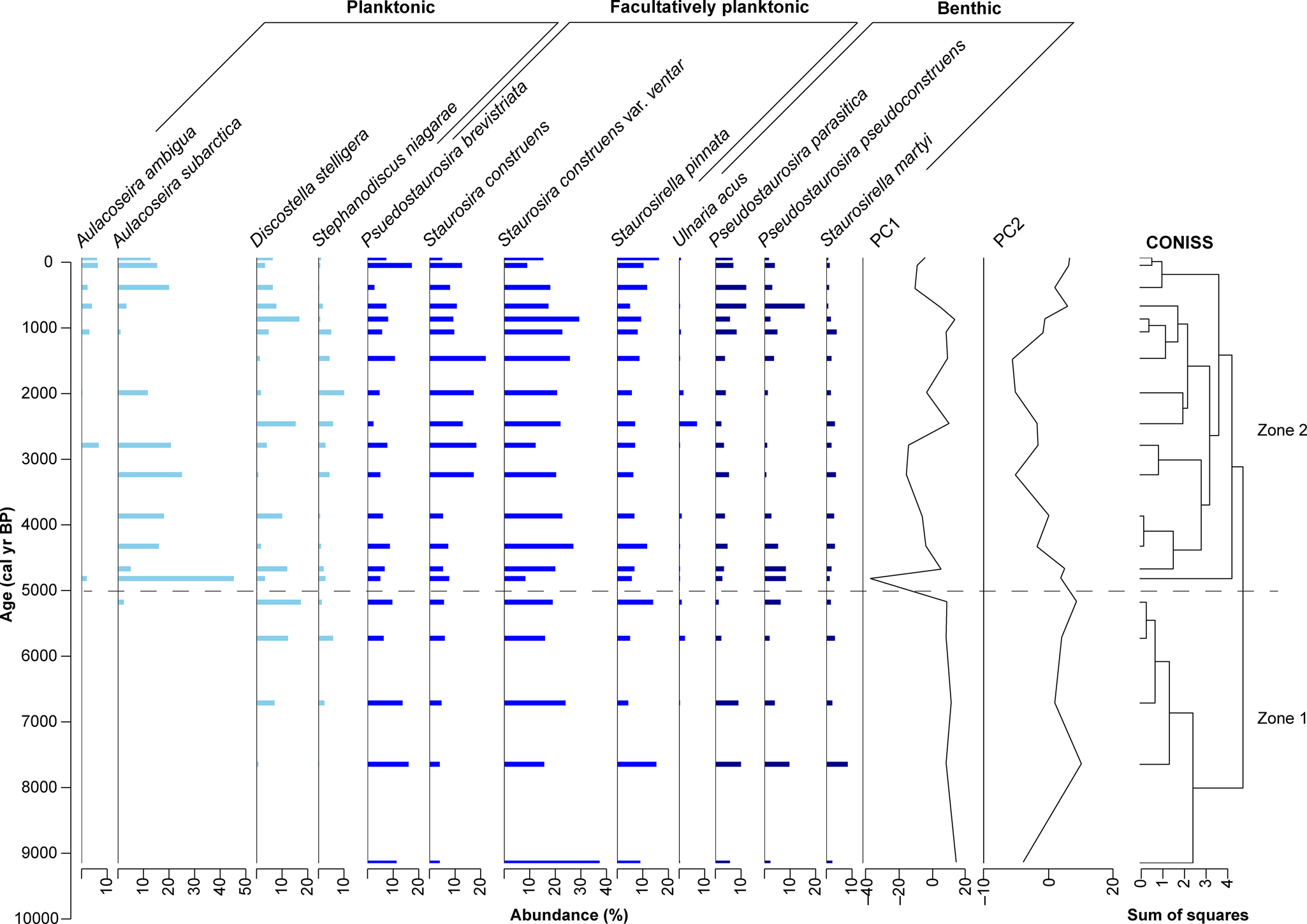
Figure 8. Relative abundances of 12 dominant diatom taxa in Kelly Lake core KLY18-2. CONISS-designated zones are indicated by the dashed line. Analyzed and plotted using the R packages Rioja (v.0.9-26; Juggins, Reference Juggins2017) and Vegan (v.2.5-7; Oksanen et al., Reference Oksanen, Kindt, Legendre, O'Hara, Henry and Stevens2007).
Zone 1 (9.2–5.0 cal ka BP; 772–543 cm)
Zone 1 is characterized by high abundances of facultatively planktonic taxa, especially Staurosira construens var. venter, and including Pseudostaurosira brevistriata, Staurosira construens, Staurosirella pinnata, and Ulnaria acus. Benthic taxa are present in relatively low abundances, including Pseudostaurosira parasitica, P. pseudoconstruens, Staurosirella martyi, and, in the most recent part of this zone, Ulnaria acus. Planktonic taxa are absent at first, although Stephanodiscus niagarae and Discostella stelligera appear in low abundances near the end of this zone, followed by Aulacoseira subarctica.
Zone 2 (5.0 cal ka BP–present; 543–0 cm)
Zone 2 features the expansion of planktonic taxa, most notably Aulacoseira subarctica. Aulacoseira ambigua makes its first appearance in this zone, though abundances remain low. Stephanodiscus niagarae and Discostella stelligera also remain present throughout this zone, with their abundances fluctuating over time. All facultatively planktonic and benthic taxa remain present throughout this zone. Facultatively planktonic diatoms, especially Staurosira construens var. venter and S. construens, are among the more prevalent taxa, whereas benthic species remain present in low abundances throughout. Toward the end of this zone, the abundances of Pseudostaurosira parasitica and P. pseudoconstruens increase.
The first two principal components (PCs) of the stratigraphic diatom assemblage data account for 65% of the overall variance in the record (λ 1 = 0.52; λ 2 = 0.13). PC1 largely tracks changes in Aulacoseira subarctica (λ 1), whereas PC2 is controlled by variations in numerous other species, most notably by the opposing relation of Discostella stelligera and Pseudostaurosira pseudoconstruens versus Staurosira construens and S. construens var. venter (Fig. 8; Supplementary Fig. 6).
Diatom oxygen isotopes
The Kelly Lake δ18Odiatom data, which cover the last ca. 9.7 cal ka BP (Fig. 4), show a range of 5.9‰ (+22.7 to + 28.6‰, n = 107), with a mean of + 27.0‰. The mean is + 24.5‰ (n = 9) prior to 7.3 cal ka BP, then shifts to + 27.6‰ (n = 83) between 7.3 cal ka BP and ca. 1960 CE, followed by a decrease to + 25.4‰ (n = 15) over the past ca. 60 years (Fig. 4). SEM images indicate that contamination by clay minerals and tephras is insignificant (e.g., Supplementary Fig. 2). EDS data reveal that the percent of Al2O3, commonly used as an indicator of siliceous clay contamination in purified biogenic silica (Brewer et al., Reference Brewer, Leng, Mackay, Lamb, Tyler and Marsh2008), is <1% in all samples. Because sedimentary diatom frustules may contain up to 1% Al2O3 incorporated into the silica matrix (Koning et al., Reference Koning, Gehlen, Flank, Calas and Epping2007), this result further indicates that samples analyzed for δ18Odiatom comprise pure biogenic silica.
Hydrologic and isotope mass balance modeling
Hydrologic and isotope mass balance calculations (Krabbenhoft et al., Reference Krabbenhoft, Bowser, Anderson and Valley1990) for the modern period suggest that groundwater inflow amounts to 1.2 × 10⁻⁴ km3/year, compared to 3.5 × 10⁻⁴ km3/year for on-lake precipitation and 2.6 × 10⁻⁴ km3/year for lake surface evaporation (Table 3). Using a fractionation factor of −0.16‰/°C between lake water (4°C) and diatom silica (Crespin et al., Reference Crespin, Sylvestre, Alexandre, Sonzogni, Pailles and Perga2010), δL for Kelly Lake in the Early Holocene (ca. 9.8–9.0 cal ka BP) was estimated to be −15.7‰, and −11.0‰ for much of the Middle and Late Holocene (ca. 7.0–0 cal ka BP) (Table 2). For these calculations (eq. 14), δ18Odiatom values were averaged over the time intervals of interest (n = 3, average = +22.9‰ for the Early Holocene; n = 80, average = +27.6‰ for the Middle to Late Holocene).
Output of the sensitivity tests reveals the quantity of Gi needed to produce our inferred (for the past) or measured (for the present) δL values in the Middle to Late Holocene (Fig. 9A–C), the Early Holocene (Fig. 9D, E), and the modern period (Fig. 9F, G). For the modern period, this output demonstrates the sensitivity of the results to the variables of interest. For past climate intervals, results reveal a range of possibilities for Gi, depending on input values for δP, and consequently δGi. Scenarios that yielded negative Gi values (indicating a net seepage from the lake to the groundwater) were considered unrealistic because the lake is known to be spring fed, therefore these were excluded from the presented results. An additional scenario is presented for the Middle to Late Holocene, where δP is elevated compared to that of modern annually averaged precipitation (Fig. 9C). This δP scenario violates the previously discussed model assumptions for both the Early Holocene and the modern time period, because inferred δL values at these times are lower than this higher δP value; this illustrates how the modeling exercise, combined with the δ18Odiatom data, provides a reasonable constraint on past δP.

Figure 9. Output of sensitivity tests conducted to investigate past hydrologic and isotope mass balance at Kelly Lake. (A–C) Middle to Late Holocene scenarios (HadCM3 4 ka snapshot). (D, E) Early Holocene scenarios (HadCM3 9 ka snapshot). (F, G) Modern scenarios. (A, D, F) Scenarios where precipitation and groundwater oxygen isotope values are lower compared with today. (B, E, G) Scenarios where precipitation and groundwater oxygen isotope values are similar to today. (C) Scenario where precipitation and groundwater oxygen isotope values are higher than today (this scenario is feasible only in the Middle to Late Holocene). Blue lines and shading show scenarios where P is 25% higher compared to the HadCM3 output; green shows P that is the same as the HadCM3 output; and pink shows P that is 25% lower. Solid blue, green, and pink lines show these P scenarios with the same evaporation rate as the HadCM3 output, whereas upper and lower bounds (dashed lines) show scenarios where E is reduced or increased 25% compared to the HadCM3 output. In all panels, the black dotted lines show the calculated groundwater inflow for the modern period (1.2 × 10⁻⁴ km3/year). The white star in (G) indicates the values of P, E, groundwater inflow, groundwater oxygen isotopes, and precipitation oxygen isotopes calculated using the modern measurements.
DISCUSSION
Controls on proxy records at Hidden and Kelly lakes
The datasets presented in this study encompass a broad array of paleoclimate proxies (chlorin, organic matter, grain size, biogenic silica, pollen, macrofossils, diatoms, and diatom oxygen isotopes), each of which reflects different aspects of past environmental conditions. By interpreting these datasets together, in two neighboring lakes with closely related environmental histories, we are able to reconstruct multiple features of regional paleoenvironmental change.
Indicators of past productivity
Chlorin is the diagenetic product of chlorophyll (Rein and Sirocko, Reference Rein and Sirocko2002), and therefore reflects changes in both terrestrial and aquatic photosynthetic organisms in the lakes and their catchments. The correlation between chlorin content at Hidden and Kelly lakes throughout the Holocene (median r = 0.64; p < 0.05 for 100% of ensembles; Figs. 3, 4; Supplementary Fig. 5) demonstrates that these data reflect processes that are not catchment specific and represent extra-local landscape patterns.
Chlorin abundance tends to be strongly related to OM fluctuations, which typically represent combined autochthonous and allochthonous OM tied to catchment-scale sediment composition and productivity (e.g., Shuman, Reference Shuman2003), changes in lake level (e.g., Digerfeldt et al., Reference Digerfeldt, Almendinger and Björck1992), or dilution by minerogenic material (e.g., Nesje and Dahl, Reference Nesje and Dahl2001). Chlorin and OM at Hidden Lake are strongly correlated (r = 0.77; p = 0.01; Fig. 3; Supplementary Fig. 4), but the two datasets do not always covary during the Holocene. In contrast, chlorin and OM at Kelly Lake are only weakly correlated (r = 0.28; p = <0.01; Fig. 4; Supplementary Fig. 4). These dissimilarities between the chlorin and OM time series at the two lakes (Figs. 3, 4; Supplementary Fig. 5) might result either from different sampling resolution at the two sites, or uncertainties in the age models. The mismatch might also result from differences in the composition or degradational state of OM, which could affect the measured RABD660;670 values, or might indicate that OM is sensitive to multiple, lake-specific processes at these sites.
BSi, in turn, might respond to a number of factors in high-latitude lakes, including length of the ice-free season (McKay et al., Reference McKay, Kaufman and Michelutti2008), nutrient availability (Perren et al., Reference Perren, Axford and Kaufman2017), dilution by minerogenic material (Krawiec and Kaufman, Reference Krawiec and Kaufman2014), or changes in water chemistry that cause dissolution (Bradbury et al., Reference Bradbury, Forester and Thompson1989). SEM imaging of diatoms in Kelly Lake sediments reveals well-preserved valves, indicating that dissolution is not a factor affecting BSi in this sequence (Supplementary Fig. 2). Fluctuations in BSi and OM at Kelly Lake are not significantly correlated at the 95% confidence level (r = 0.22; p = 0.12; Fig. 4; Supplementary Fig. 4), indicating either that changes in BSi at this site might be uncoupled from allochthonous OM inputs, or that BSi reflects processes that affect diatoms directly, such as changes in seasonality (Buczkó et al., Reference Buczkó, Szurdoki, Braun and Magyari2018) or taxon-specific responses of diatoms to changing climate or environmental conditions (Lotter and Hofmann, Reference Lotter, Hofmann and Tonkov2003). However, chlorin and BSi at Kelly Lake are moderately correlated (r = 0.40; p < 0.01; Fig. 4; Supplementary Fig. 4), indicating that BSi (dominantly composed of diatoms at this site) is an important component of total chlorophyll production in the lake and its catchment, and that BSi is influenced by at least some of the same climate variables that drive overall productivity at both lakes. Similar to diatom abundance (as reflected by BSi), the abundance of bryozoan statocysts in lake sediment can indicate past productivity, where more statocysts occur with higher concentrations of nutrients in the lake water (Crisman et al., Reference Crisman, Crisman and Binford1986; Hartikainen et al., Reference Hartikainen, Johnes, Moncrieff and Okamura2009).
Indicators of past vegetation change
Productivity also can be influenced by changes in plant community composition in the Hidden Lake and Kelly Lake catchments. For example, Alnus is known to increase local nitrogen availability (Shaftel et al., Reference Shaftel, King and Back2011), and its arrival has been shown to drive increases in BSi at nearby Sunken Island Lake (Broadman et al., Reference Broadman, Kaufman, Henderson, Berg, Anderson, Leng, Stahnke and Muñoz2020) and in southwestern Alaska at Farewell Lake (Hu et al, Reference Hu, Finney and Brubaker2001) and Lone Spruce Pond (Kaufman et al., Reference Kaufman, Axford, Anderson, Lamoureux, Schindler, Walker and Werner2012). These fluctuations in nutrient content associated with shifts in vegetation can also drive changes in diatom assemblages because some diatom species respond strongly to the presence of certain nutrients (e.g., Perren et al., Reference Perren, Axford and Kaufman2017).
Whereas pollen data tend to reflect regional vegetation changes, plant macrofossil data more closely reflect the taxa immediately surrounding the lake (e.g., Jackson et al., Reference Jackson, Booth, Reeves, Anderson, Minckley and Jones2014). Therefore, the presence of Picea, Alnus, and Betula macrofossils in Kelly Lake sediments confirm the presence of these taxa in the immediate vicinity of this site, while the Hidden Lake pollen record indicates the presence of these taxa over a broader region.
Indicators of past hydroclimate
Several indicators analyzed in this study are commonly used to reconstruct past hydroclimate conditions. For example, the presence of some micro- and macrofossils can indicate changes in lake level, including oospore macrofossils associated with Characean algae (Chara sp.). Chara is a genus of photosynthetic macrophyte that dwells in shallow, clear waters (typically ~1–3 m water depth; Pukacz et al., Reference Pukacz, Pełechaty and Frankowski2016). Large quantities of Chara oospores in lake sediment have been associated with dense meadows of Chara proximal to the site sampled (Zhao et al., Reference Zhao, Sayer, Birks, Hughes and Peglar2006; Ayres et al., Reference Ayres, Sayer, Skeate and Perrow2007), and with the persistent presence of Chara over prolonged time periods (Van den Berg et al., Reference Van den Berg, Coops and Simons2001). Therefore, an increase in the abundance of Chara oospores in Kelly Lake sediments indicates that these algae were more abundant near the coring site at the lake's depocenter. Simple bathymetric modeling (Supplementary Fig. 3) reveals that a decrease in lake level would shift shallower waters closer to this coring site. Therefore, an increase in the concentration of oospores likely reflects a lower lake level at Kelly Lake.
Similarly, the concentration of bryozoan statocysts can indicate lake level. Bryozoans attach themselves to logs and aquatic macrophytes (Francis, Reference Francis, Smol, Birks and Last2001; Wood, Reference Wood, Thorp and Covich2001), and therefore an increase in the concentration of statocysts may reflect a lower lake level at Kelly Lake. An increased concentration of statocysts also can be interpreted to indicate the presence of flowing surface or spring water, which is often (but not always) associated with shallow water (Francis, Reference Francis, Smol, Birks and Last2001; Wood, Reference Wood, Thorp and Covich2001). Diatom assemblages can provide yet another line of evidence for lake level fluctuations, where an increase in the relative abundance of planktonic diatom taxa can indicate a rise in lake level that creates additional habitat for these diatoms (Wolin and Duthie, Reference Wolin, Duthie, Smol and Stoermer1999).
These inferred lake level changes can be interpreted to reflect changes in hydroclimate. For example, a rise in inferred lake level might indicate an increased contribution of groundwater (e.g., from melting glaciers), or an increase in the amount of precipitation relative to evaporation (increased P-E). Precipitation rate and P-E, in turn, are strongly influenced in this region by the strength of the Aleutian Low, where a stronger pressure cell typically results in increased storminess and generally wetter winters in southern Alaska (Rodionov et al., Reference Rodionov, Bond and Overland2007).
δ18Odiatom is also sensitive to changes in past hydroclimate. The temperature-dependent fractionation between diatom silica and lake water is relatively small, meaning it is often overwhelmed by larger fluctuations in δL that can occur due to changes in P-E, δP, or other changes in lake hydrology (see Leng and Barker, Reference Leng and Barker2006) for a summary of the influences on δ18Odiatom). This is particularly relevant in the North Pacific region, where relatively large magnitude changes in both P-E and δP have been documented during the Holocene. Therefore, δ18Odiatom from Kelly Lake is interpreted primarily in terms of hydroclimatic variables, as has been done for other δ18Odiatom records from southern Alaska (Schiff et al., Reference Schiff, Kaufman, Wolfe, Dodd and Sharp2009; Bailey et al., Reference Bailey, Kaufman, Henderson and Leng2015, Reference Bailey, Kaufman, Sloane, Hubbard, Henderson, Leng, Meyer and Welker2018; Broadman et al., Reference Broadman, Kaufman, Henderson, Berg, Anderson, Leng, Stahnke and Muñoz2020), rather than in terms of Holocene temperature changes.
While P-E and evaporative isotope enrichment are major influences on δL in many closed-basin lakes (e.g., Broadman et al., Reference Broadman, Kaufman, Henderson, Berg, Anderson, Leng, Stahnke and Muñoz2020), several lines of evidence suggest their influence at Kelly Lake is minimal in recent years compared with nearby lakes. First, according to a survey of regional water isotopes (Broadman et al., Reference Broadman, Kaufman, Henderson, Berg, Anderson, Leng, Stahnke and Muñoz2020), modern δL at Kelly Lake (−13.9‰ VSMOW; n = 7) is only slightly elevated above that of local rivers (−14.8‰ and −16.6‰ for the Moose and Kenai rivers), regional groundwater (−16.5‰), and the precipitation-weighted annual average of regional precipitation (−17.7‰, recorded in Anchorage from 2005–2018; Bailey et al., Reference Bailey, Klein and Welker2019). In contrast, δL at many closed-basin lakes in the Kenai lowlands ranges from −10‰ to −6‰ (Fig. 2B). Second, δ18Odiatom values have decreased in recent decades (upper 18 cm of sediment), while annual temperature has increased (Fig. 10H) and average annual precipitation rates have remained constant or slightly decreased since 1940 CE (see data for Kenai airport at https://akclimate.org/data/data-portal/). Were δ18Odiatom sensitive to P-E, this would be the opposite of the pattern that would be expected, because rising temperature leads to increased evaporation, a phenomenon that was documented in the most recent sediments of nearby Sunken Island Lake (Broadman et al., Reference Broadman, Kaufman, Henderson, Berg, Anderson, Leng, Stahnke and Muñoz2020).
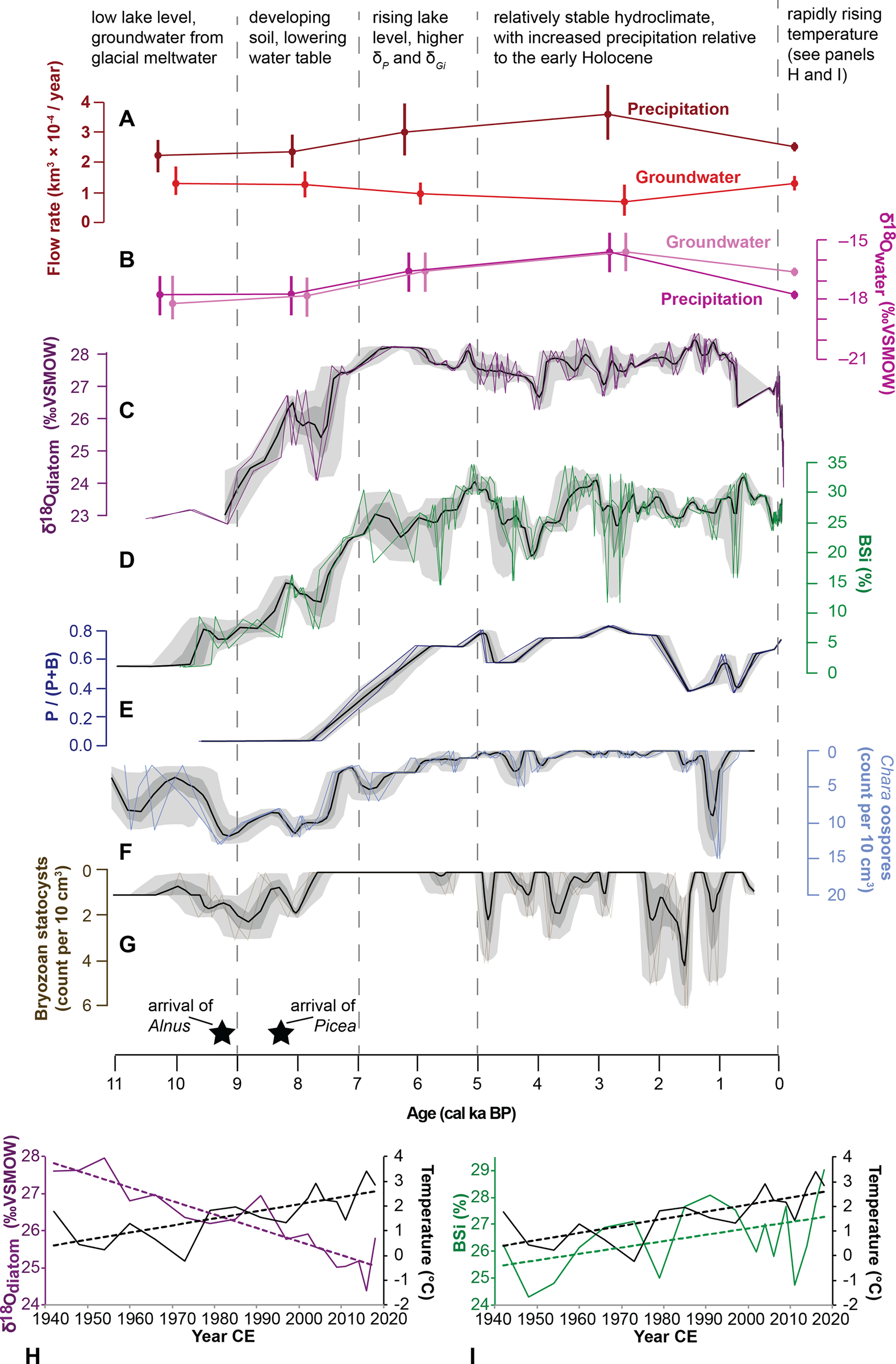
Figure 10. Summary of key hydroclimate indicators from Hidden and Kelly Lakes. (A, B) Most plausible modeled scenarios (Fig. 9) for each time period for: (A) rates of groundwater inflow and precipitation, and (B) oxygen isotope composition for each of these hydrologic inputs to Kelly Lake. Vertical bars are uncertainty estimates, some of which are based on measurements, and some of which are simulated or inferred. (C–G) Ribbon plots of proxy data from Kelly Lake; black lines are the mean of the age model ensembles, dark- and light-gray shading encompass 68% and 95% of the ensemble members, respectively; colored lines show five representative members of the age model ensemble. Ribbon plots show the following datasets: (C) δ18Odiatom (‰ VSMOW); (D) BSi (%); (E) proportion of planktonic diatoms, calculated as the number of planktonic diatoms (P) divided by the sum of all planktonic and benthic diatoms (P + B); (F) concentration of Chara oospores (count per 10 cm3); and (G) concentration of bryozoan statocysts (count per 10 cm3); the first occurrences of Alnus and Picea macrofossils at Kelly Lake are shown (black stars). (H) Temperature at Kenai airport (black) shown with Kelly Lake δ18Odiatom (purple) data from 1944–2018 CE, with linear trend lines. (I) Temperature at Kenai airport (black) shown with Kelly Lake BSi (green) abundance from 1944–2018 CE, with linear trend lines. The age-uncertain correlations for data in B and C are shown in Supplementary Figure 5.
Another factor influencing δL at Kelly Lake is change in the flux and isotope composition of groundwater (Gi and δGi). Several lines of evidence suggest that Gi is an important component of Kelly Lake's hydrological budget, including the presence of visibly discharging subaqueous springs, and a substantial contribution of Gi calculated in the mass balance model output for the modern period (Fig. 9G). In the Kenai lowlands there are two possible sources for Gi: a surficial aquifer and a deep aquifer (Eilers et al., Reference Eilers, Landers, Newell, Mitch, Morrison and Ford1992). Geochemical evidence from a survey of lakes in the Kenai lowlands suggests that lakes fed by the deep aquifer have higher alkalinity and total dissolved solids (TDS) compared with lakes fed by the surficial aquifer (Eilers et al., Reference Eilers, Landers, Newell, Mitch, Morrison and Ford1992). The presence of carbonate muds (marl) during the late glacial and Early Holocene, as well as relatively high values for limnological indicators analyzed at Kelly Lake in June 2021 (pH: 7.8; conductivity: 144 μm; alkalinity: 62 ppm; total hardness: 62 ppm) suggest that Kelly Lake is fed by relatively deep groundwater. Furthermore, similar but slightly higher values for all indicators analyzed at Hidden Lake (pH: 8.3; conductivity: 183 μm; alkalinity: 75 ppm; total hardness: 78 ppm) indicate this groundwater might travel to Kelly Lake via Hidden Lake. Deep groundwater is likely recharged by snowmelt at high altitudes in the Kenai Mountains, and thus is primarily fed by winter season precipitation, which has low δ18O (Fig. 2A). In addition to climatic fluctuations that could influence Gi, groundwater sourced from a deep aquifer also could be influenced by tectonic activity because Kelly Lake is located proximal to a fault that lies along the mountain front (Karlstrom, Reference Karlstrom1964). The influence of tectonism on groundwater discharge has been demonstrated at other lakes adjacent to fault zones (e.g., Hosono et al., Reference Hosono, Yamada, Manga, Wang and Tanimizu2020; Ide et al., Reference Ide, Hosono, Kagabu, Fukamizu, Tokunaga and Shimada2020).
It is also possible that Kelly Lake is fed by surficial groundwater, which is likely recharged in part by glacier meltwater. Studies examining glacier retreat during recent decades have demonstrated that the meltwater generated by receding glaciers can recharge a surface aquifer and form an important component of lowland river discharge, even as glacier ice retreats into the mountains (e.g., Liljedahl et al., Reference Liljedahl, Gädeke, O'Neel, Gatesman and Douglas2017). Continental ice tends to incorporate primarily snowfall that fell at high elevation (Fig. 2A), and therefore glacier ice can be expected to have relatively low δ18O (e.g., Bhatia et al., Reference Bhatia, Das, Kujawinski, Henderson, Burke and Charette2011). Therefore, during periods of glacial retreat, it is likely that surficial groundwater in the Kenai lowlands would have relatively low δ18O. If Kelly Lake is currently or was previously fed by the surficial aquifer, glacial meltwater might contribute substantially to Gi at this site during periods of glacier retreat. However, a physical connection between the surficial aquifer and the Kelly Lake subaqueous springs remains uncertain, limiting our ability to definitively identify the source of Gi (surficial or deep).
Regardless of the mechanism(s) influencing Gi at this site, it is likely that δGi at Kelly Lake would be relatively low, both now and in the past, because both the deep and surficial groundwater in the region are recharged by sources at high elevations that dominantly incorporate winter precipitation. This is supported by the δ18O of local well water (−16.5‰), which is lower than the modern δL of Kelly Lake (−13.9‰) (Fig. 2B; Broadman et al., Reference Broadman, Kaufman, Henderson, Berg, Anderson, Leng, Stahnke and Muñoz2020). Therefore, increased Gi would likely decrease δL at Kelly Lake.
Both δGi and δL are also sensitive to changes in δP, which is influenced by seasonal changes in air temperature (Dansgaard, Reference Dansgaard1964) (Fig. 2A) and the trajectories of storms that deliver precipitation (e.g., Bailey et al., Reference Bailey, Kaufman, Henderson and Leng2015). In south-central Alaska, summer season (JJA) precipitation tends to have higher δP values, whereas the winter season (DJF) has lower δP (Fig. 2A). Therefore, a shift in the seasonality of precipitation (e.g., a larger proportion of annual precipitation falling in the summer) would influence annually weighted δP, as well as the contribution of δGi derived from recent precipitation, and would subsequently change δL.
The other important influences on δP in this region are the source area and trajectory of storms, which are controlled by the position and intensity of the Aleutian Low (AL). Because a strong AL encourages south-to-north (meridional) transport from the Gulf of Alaska to the Kenai lowlands (Cayan and Peterson, Reference Cayan, Peterson and Peterson1989; Mock et al., Reference Mock, Bartlein and Anderson1998; Rodionov et al., Reference Rodionov, Bond and Overland2007; Berkelhammer et al., Reference Berkelhammer, Stott, Yoshimura, Johnson and Sinha2012), storms associated with a strong AL tend to travel less distance and cross fewer continental barriers before arriving in the Kenai lowlands. Conversely, a weak AL encourages west-to-east (zonal) transport from farther west in the North Pacific Ocean. Storms during a weak AL tend to travel greater distances and cross more continental barriers, and therefore are likely to experience more rain-out of 18O, depleting δP arriving in the Kenai lowlands. This relationship between the AL and δP has been corroborated by several isotope-enabled model experiments (Berkelhammer et al., Reference Berkelhammer, Stott, Yoshimura, Johnson and Sinha2012; Porter et al., Reference Porter, Pisaric, Field, Kokelj, deMontigny, Healy and LeGrande2014).
In contrast, some authors have suggested the opposite relationship, where a stronger AL results in lower δP. However, studies that invoke this opposing relationship between δP and AL strength have attributed it to unique characteristics of their study sites, such as a strong rain-out effect (Anderson et al., Reference Anderson, Abbott, Finney and Burns2005), high altitude (Fisher et al., Reference Fisher, Osterberg, Dyke, Dahl-Jensen, Demuth, Zdanowicz and Bourgeois2008), or sensitivity to summer conditions (Jones et al., Reference Jones, Wooller and Peteet2014). Furthermore, the limited available modern δP data from Anchorage (Bailey et al., Reference Bailey, Klein and Welker2019) indicates that stronger AL years between 2005 and 2018 had higher δP than weak AL years (Broadman et al., Reference Broadman, Kaufman, Henderson, Berg, Anderson, Leng, Stahnke and Muñoz2020). Therefore, we interpret that a stronger AL most likely results in higher δP values on decadal to multi-millennial timescales at our site. However, the relationship between the AL and δP is superimposed on other hydroclimatic influences (e.g., P-E, seasonality, melting glacier ice), making it difficult to disentangle the influence of AL behavior both in modern δP (Bailey et al., Reference Bailey, Klein and Welker2019) and in paleo oxygen isotope datasets (Broadman et al., Reference Broadman, Kaufman, Henderson, Berg, Anderson, Leng, Stahnke and Muñoz2020) in this region.
As a result of the presence of multiple hydroclimatic variables that influence δL and δ18Odiatom at Kelly Lake, the scenarios simulated with the mass balance model include a range of possible values for δP, δGi, P, and E (Fig. 9A–E). By modeling sensitivity of the system to ranges of values for all these variables, we are able to assess their influence on changes to Gi.
Deglacial and Holocene landscape, vegetation, and hydroclimatic change
Deglaciation and the earliest Holocene (ca. 13.1–9.0 cal ka BP)
The new age model presented in this study places the transition from glaciolacustrine sediments to gyttja in Hidden Lake (Fig. 3) at ca. 13.1 cal ka BP, ca. 3500 years later than suggested by the previously acquired radiocarbon age (Ager, Reference Ager and Wright1983). This stratigraphic transition is associated with retreat of glaciers from the Hidden Lake catchment, and previously has been cited as the termination of the Skilak stade of the Naptowne glaciation, with the Elmendorf stade following shortly thereafter (Fig. 1C; Reger et al., Reference Reger, Sturmann, Berg and Burns2007). Moraines previously thought to correlate with the Elmendorf stade lie immediately up valley from Hidden Lake (Fig. 1C; Reger et al., Reference Reger, Sturmann, Berg and Burns2007). However, the absence of glaciolacustrine deposits in the Hidden Lake sediments after ca. 13.1 cal ka BP suggests these presumed Elmendorf-age moraines were formed earlier. A recently revised chronology of the Elmendorf moraine near Anchorage suggests that ice receded from the Matanuska and Knik valleys in two stages: the first between ca. 16.8–16.4 cal ka BP, and the second concluding by ca. 13.7 cal ka BP (Kopczynski et al., Reference Kopczynski, Kelley, Lowell, Evenson and Applegate2017). It is possible the moraines in our study region (Fig. 1C) represent a similar progression of events, with the second phase of ice retreat concluding by ca. 13.1 cal ka BP, ending the deposition of glaciolacustrine sediment at Hidden Lake. Because the recovered Hidden Lake sediments terminate in glaciolacustrine silt and sand (rather than till or bedrock), we cannot definitively say whether these sediments at the ca. 13.1 cal ka BP age correspond to termination of the Skilak stade, or a time period thereafter when glaciers were upvalley in Hidden Lake's catchment.
Though a vegetation transition occurs during the Younger Dryas, characterized by a rise in Betula and a decrease in Cyperaceae (Fig. 6), there is no evidence for a substantial climate perturbation reflected in the Hidden Lake sedimentological indicators at this time. Therefore, if glaciers in the Kenai Mountains advanced during the Younger Dryas, they were not extensive enough to re-encroach into the Hidden Lake catchment. It is also possible that the influence of groundwater sourced from retreating glaciers at this location near the Kenai Mountains would mask changes documented at nearby sites during the Younger Dryas, as these fluctuations are mostly associated with precipitation and/or atmospheric circulation patterns (e.g., Yu et al., Reference Yu, Walker, Evenson and Hajdas2008; Kaufman et al., Reference Kaufman, Anderson, Hu, Berg and Werner2010; Broadman et al., Reference Broadman, Kaufman, Henderson, Berg, Anderson, Leng, Stahnke and Muñoz2020).
As arboreal taxa increased from ca. 12.8–9.3 ka cal BP following the retreat of glaciers (Figs. 6, 7), charcoal in the Kelly Lake sediment sequence (Fig. 7) indicates the occurrence of fire that accompanied these developing forests (e.g., Anderson et al., Reference Anderson, Hallett, Berg, Jass, Toney, de Fontaine and DeVolder2006), likely driven in part by warmer summer temperatures (Clegg et al., Reference Clegg, Kelly, Clarke, Walker and Hu2011). Throughout this interval, sediments are composed of interbedded gyttja and gray silt and clay (Fig. 3). These lines of evidence coupled with low values for productivity proxies (chlorin and OM; Fig. 3) suggest a postglacial landscape characterized by low productivity, potentially driven by relatively cool temperatures caused by cold, glacially derived groundwater inputs.
The oldest sediments in Kelly Lake core KLY18-2, which span ca. 10.7–9.2 cal ka BP, are rich in both OM and carbonate (see Wrobleski, Reference Wrobleski2021, for a detailed description of the carbonate deposits at Kelly Lake). The presence of numerous Chara oospores (Figs. 4, 7, 10F) indicates that at least some of the carbonate production at this time was Chara-mediated. This profusion of oospores also suggests that Chara plants were present in high abundances near the coring location at this time (Zhao et al., Reference Zhao, Sayer, Birks, Hughes and Peglar2006). The abundance of Chara oospores also indicates that Kelly Lake's water level was lower than present, including at the coring location (Supplementary Fig. 3), because the distribution of Chara species in a lake is typically limited to shallow waters (Pukacz et al., Reference Pukacz, Pełechaty and Frankowski2016). The presence of bryozoan statocysts in the macrofossil assemblage at this time also suggests low lake level (Francis, Reference Francis, Smol, Birks and Last2001; Wood et al., Reference Wood, Thorp and Covich2001).
These findings are consistent with evidence for lowered lake level in the Early Holocene based on dated transitions between minerogenic sediments and terrestrial peat at Sunken Island Lake, 28 km to the northwest (Broadman et al., Reference Broadman, Kaufman, Henderson, Berg, Anderson, Leng, Stahnke and Muñoz2020; Berg et al., Reference Berg, Kaufman, Anderson, Wiles, Lowell, Mitchell, Hu and Wernerin press). In light of these lines of evidence, in our sensitivity tests for this climate interval, we estimate that Kelly Lake's water level and surface area were reduced, but were still high enough to account for the continuous sediment deposition observed at the coring site of KLY18-4 (Fig. 1D; Table 2; Supplementary Fig. 3). High OM, but low chlorin and BSi, might indicate low productivity in the lake, but with significant allochthonous organic inputs from the Betula-dominated hardwood forest, as indicated by the Kelly Lake macrofossil data (Fig. 7) and the Hidden Lake pollen data (Fig. 6). The oldest sample with well-preserved diatoms at ca. 9.2 cal ka BP is dominated by facultatively planktonic taxa, which previously have been shown to thrive in Early Holocene Arctic lakes, possibly due to elevated summer air temperature (Finkelstein and Gajewski, Reference Finkelstein and Gajewski2008).
The oldest δ18Odiatom samples, from ca. 9.7–9.2 cal ka BP, have the lowest values recorded in the time series (mean = +22.9‰, n = 3), indicating a commensurately low δL value (~ −15.7‰; Table 2). Hydrologic and isotope mass balance modeling suggests two δP scenarios that could result in this δL value: (1) low δP, which might reflect either a weaker AL or a greater annual contribution of winter season precipitation, and less groundwater inflow (Fig. 9D); or (2) δP values similar to today's, with similar or larger groundwater inflows (Fig. 9E). Paleoclimate reconstructions also generally indicate δP lower than or similar to modern in the Early Holocene (Jones et al., Reference Jones, Wooller and Peteet2014, Reference Jones, Anderson, Keller, Nash, Littell, Wooller and Jolley2019; Bailey et al., Reference Bailey, Kaufman, Sloane, Hubbard, Henderson, Leng, Meyer and Welker2018).
While it is not possible to definitively exclude any of these scenarios, it is most likely that δP was similar to today (−17.7‰; Bailey et al., Reference Bailey, Klein and Welker2019), and Gi was similar to its current rate (Fig. 9E). In modeled scenarios where δP is substantially lower compared to today (Fig. 9D), P must be ~25% lower (or evaporation must be ~25% higher) than that simulated by HadCM3. The 9 ka snapshot already simulates a ~15% decrease in P during the Early Holocene relative to the modern period (Table 3), and it is unlikely that P would be reduced an additional 25% compared to the model simulation. A scenario with lower δP also would require much lower Gi compared to today (Fig. 9D), which is unlikely given the recently deglaciated landscape and likely continued contribution of glacially derived water. Therefore, it is most likely that δP was similar to that of today, P was similar to or slightly reduced from the Early Holocene model simulated value, and Gi was similar to that of today (Figs. 9E, 10A–C). δGi was probably similar to or lower than δP, potentially due to an elevated contribution of meltwater from snow or glacier ice recharging Kenai lowland aquifers following deglaciation (Figs. 9E, 10A–C).
The Early to Middle Holocene transition (ca. 9.0–7.0 cal ka BP)
After the postglacial period characterized by low lake level, groundwater likely sourced from glacial meltwater, and relatively low lacustrine productivity, the following two millennia were transformative. At Kelly Lake, BSi increases over this interval (Fig. 4), coincident with the expansion and dominance of Alnus in the region, with the highest relative abundances at ca. 9.3–8.6 cal ka BP (Figs. 6, 10D). The increase in BSi might be driven by the presence of Alnus in the Kelly Lake catchment, resulting in nitrogen fixation, more available nitrogen, and consequent diatom blooms (e.g., Perren et al., Reference Perren, Axford and Kaufman2017; Broadman et al., Reference Broadman, Kaufman, Henderson, Berg, Anderson, Leng, Stahnke and Muñoz2020). Though Alnus macrofossils do not appear in the Kelly Lake sediments until ca. 8.2 cal ka BP (Fig. 7), the regional increase in Alnus (Fig. 6) coupled with the increase in BSi (Fig. 10D) indicates a relationship between the two at Kelly Lake. The diatom assemblage remains dominated by facultatively planktonic taxa (Fig. 8), and Chara oospores and bryozoan statocysts remain relatively abundant (Fig. 10F, G), suggesting there was little change in lake level over this interval.
δ18Odiatom increases over this interval by ~5‰ (from + 22.9‰ prior to 9 cal ka BP to + 27.9‰ during the two millennia starting at 7 cal ka BP), indicating a transition either in the lake's hydrologic inputs (e.g., precipitation or groundwater) or in regional hydroclimate. The cause of the transition between ca. 9–7 cal ka BP is likely associated with a change in Gi and δGi, potentially due to the decreased influence of meltwater from retreated glaciers by ca. 7 cal ka BP. Because Kelly Lake lies close to the mountains (Fig. 1C), it might be more strongly influenced by glacier melt compared with sites further north or west in the Kenai lowlands. Kelly Lake's proximity to the mountains relative to these other sites might explain the lack of evidence for a shift in hydrology or hydroclimate at this time in nearby oxygen isotope reconstructions (e.g., Jones et al., Reference Jones, Wooller and Peteet2014, Reference Jones, Anderson, Keller, Nash, Littell, Wooller and Jolley2019; Broadman et al., Reference Broadman, Kaufman, Henderson, Berg, Anderson, Leng, Stahnke and Muñoz2020). This possibility is supported by the Middle to Late Holocene model scenarios, which require lower Gi compared to the present (Fig. 9A–C).
The diminished influence of groundwater would have resulted in a lower water table and less saturated soils, which might help explain the establishment and expansion of Picea near Hidden and Kelly lakes in the Early Holocene. Picea glauca (white spruce) is the Picea species that most likely arrived initially, as documented in many nearby locations at this time (Anderson et al., Reference Anderson, Hallett, Berg, Jass, Toney, de Fontaine and DeVolder2006, Reference Anderson, Kaufman, Berg, Schiff and Daigle2017, Reference Anderson, Berg, Williams and Clark2019). The first occurrence of Picea macrofossils at Kelly Lake (ca. 8.2 cal ka BP; Fig. 7) occurs approximately concurrent with that recorded at other locations in the Kenai lowlands, suggesting that migration of P. glauca is regionally consistent; however, the transition to a Picea-dominated forest (by ca. 8.0 cal ka BP; Fig. 6) occurs substantially earlier (e.g., Anderson et al., Reference Anderson, Hallett, Berg, Jass, Toney, de Fontaine and DeVolder2006, Reference Anderson, Kaufman, Berg, Schiff and Daigle2017, Reference Anderson, Berg, Williams and Clark2019). Picea glauca does not tolerate saturated soils (Landhausser et al., Reference Landhausser, Silins, Lieffers and Liu2003), and it has been suggested that it will not become established until soil properties, including soil moisture, are sufficient for it to succeed (Henne et al., Reference Henne, Elkin, Reineking, Bugmann and Tinner2011). Therefore, the relatively early transition to a Picea-dominated forest might be explained in part by a shift in soil properties (i.e., less water-logged soils) driven by a reduction in Gi. Once established, P. glauca likely affected soil properties (Messender, Reference Messender1980; Ranger and Nys, Reference Ranger and Nys1994; Orlova et al., Reference Orlova, Lukina, Smirnov and Artemkina2016), potentially creating a positive feedback between Picea expansion and soil development.
Rising lake level during the Middle Holocene (ca. 7.0–5.0 cal ka BP)
Following the preceding transition in lake hydrology and soil development, proxy data suggest lake level at Kelly Lake may have risen from ca. 7.0– 5.0 cal ka BP, in agreement with conclusions based on other sites in this region (Kaufman et al., Reference Kaufman, Axford, Henderson, McKay, Oswald, Saenger and Anderson2016; Broadman et al., Reference Broadman, Kaufman, Henderson, Berg, Anderson, Leng, Stahnke and Muñoz2020; Berg et al., Reference Berg, Kaufman, Anderson, Wiles, Lowell, Mitchell, Hu and Wernerin press). While most sedimentological data indicate little change occurred at this time (Figs. 3, 4), by 5 cal ka BP there is an increase in the proportion of planktonic diatoms (Fig. 10E), which might reflect an increase in available water column habitat caused by rising lake level (Wolin and Duthie, Reference Wolin, Duthie, Smol and Stoermer1999). At the same time, concentrations of Chara oospores and bryozoan statocysts decline, with low concentrations prevailing during the Late Holocene starting at ca. 5 cal ka BP (Fig. 10F, G). While likely related to rising lake level, we suggest that the decline of Chara might also have been driven by a decrease in pH associated with establishment of coniferous forest. Following these lines of evidence, and because satellite imagery reveals that lake level was higher compared to modern conditions at some point in the past (Supplementary Fig. 3), sensitivity tests for the Middle to Late Holocene (Fig. 9A–C) assume lake level was slightly higher compared to modern conditions.
δ18Odiatom (average = +27.9‰, n = 14) and inferred δL values are elevated compared to previous millennia, and fluctuate relatively little over this 2000 year period, despite evidence for rising lake level. Due to the diminished influence of groundwater sourced from retreating glaciers, the dominant controls on δL likely shifted to P, E, and δP. Results of the sensitivity tests suggest that high δL could plausibly have resulted from δP either higher than (Fig. 9C) or similar to (Fig. 9B) that of today. A scenario with higher δP requires wetter conditions than simulated by HadCM3 (Fig. 9C), whereas scenarios with lower δP require drier conditions (Fig. 9A, B). Reconstructions from nearby sites suggest δP remained relatively low at ca. 7 cal ka BP, but increased by ca. 5–4 cal ka BP (Jones et al., Reference Jones, Wooller and Peteet2014, Reference Jones, Anderson, Keller, Nash, Littell, Wooller and Jolley2019; Bailey et al., Reference Bailey, Kaufman, Sloane, Hubbard, Henderson, Leng, Meyer and Welker2018; Broadman et al., Reference Broadman, Kaufman, Henderson, Berg, Anderson, Leng, Stahnke and Muñoz2020). A synthesis of hydroclimate records from this region also indicates that southern Alaska became wetter during the Late Holocene, compared with a relatively drier Middle Holocene (Kaufman et al., Reference Kaufman, Axford, Henderson, McKay, Oswald, Saenger and Anderson2016). Therefore, it is likely that δP was similar to modern, and P was relatively low at ca. 7 cal ka BP, but that both began to increase by ca. 5 cal ka BP (Figs. 9C, 10A–C).
High lake level and relative stability during the Late Holocene (ca. 5.0–0 cal ka BP)
Relatively high δP and increased P (Fig. 9C) likely persisted for much of the Late Holocene. δ18Odiatom values during the most recent ca. 5 cal ka BP exhibit relatively little variability (mean = +27.6‰; n = 66), and inferred lake level is stable compared to previous millennia (Figs. 4, 10E–G). Continued relatively high δ18Odiatom (and therefore δL) over this time period might be driven by increased δP associated with a strengthened AL, which has been documented in previous studies to begin at ca. 5.5–4.5 cal ka BP (Jones et al., Reference Jones, Wooller and Peteet2014, Reference Jones, Anderson, Keller, Nash, Littell, Wooller and Jolley2019; Bailey et al., Reference Bailey, Kaufman, Sloane, Hubbard, Henderson, Leng, Meyer and Welker2018; Broadman et al., Reference Broadman, Kaufman, Henderson, Berg, Anderson, Leng, Stahnke and Muñoz2020; Du et al., Reference Du, Hendy, Hinnov, Brown, Zhu and Poulsen2020).
An increase in the abundance of both BSi and bryozoan statocysts (Fig. 10D, G) at this time might indicate increased productivity and nutrient concentrations in Kelly Lake (Crisman et al., Reference Crisman, Crisman and Binford1986; Hartikainen et al., Reference Hartikainen, Johnes, Moncrieff and Okamura2009; Perren et al., Reference Perren, Axford and Kaufman2017). Additionally, the increased concentration of bryozoan statocysts and, to a lesser extent, Chara oospores (Fig. 10F, G), might have resulted from an increase in lake level that inundated the shallowest area of Kelly Lake (Supplementary Fig. 3), creating additional habitat for these organisms that are limited to shallow waters (Francis, Reference Francis, Smol, Birks and Last2001; Wood, Reference Wood, Thorp and Covich2001; Pukacz et al., Reference Pukacz, Pełechaty and Frankowski2016). Composition of the surrounding vegetation (Figs. 6, 7) and indicators of both productivity (Figs. 3, 4) and lake level (Fig. 10E–G) remain relatively stable throughout the Late Holocene.
Whereas many paleo isotope datasets from southern Alaska show one of the largest step-shifts and/or changes in variability during the Middle to Late Holocene transition, or during the Late Holocene (e.g., Schiff et al., Reference Schiff, Kaufman, Wolfe, Dodd and Sharp2009; Jones et al., Reference Jones, Wooller and Peteet2014, Reference Jones, Anderson, Keller, Nash, Littell, Wooller and Jolley2019; Bailey et al., Reference Bailey, Kaufman, Sloane, Hubbard, Henderson, Leng, Meyer and Welker2018; Broadman et al., Reference Broadman, Kaufman, Henderson, Berg, Anderson, Leng, Stahnke and Muñoz2020), this is not the case for Kelly Lake. Here, the largest step shift prior to the instrumental period occurs from the Early to Middle Holocene (Fig. 10C). This pronounced difference might indicate the importance of Gi and δGi in influencing δL at Kelly Lake, due to its location adjacent to mountains and glaciers. Furthermore, the Kelly Lake proxy data do indicate that lake level increased by ca. 5 cal ka BP, suggesting a hydroclimatic and/or hydrologic shift may have occurred at this time (Fig. 10E–G), likely associated with shifts in P, E, and δP (rather than by changes in Gi and δGi). Overall, it is most likely that the influence of a strengthened AL by ca. 5–4 cal ka BP that dominates the Holocene oxygen isotope datasets from several nearby sites is subdued in this δ18Odiatom dataset due to Kelly Lake's hydrologic setting.
Abrupt change in recent decades (1950 CE–present)
While most datasets analyzed in this study do not extend through recent decades, or do not have sufficient temporal resolution to examine trends over the instrumental period, both BSi and δ18Odiatom values at Kelly Lake do have sufficient resolution for this, and show abrupt changes since ca. 1950 CE. Specifically, BSi increases from 1944–2018 CE (average = 26.7%, n = 16; Fig. 10I), whereas δ18Odiatom decreases over this time period, to values approaching those of the earliest Holocene (average = +25.5‰, n = 16; Fig. 10H). These trends in δ18Odiatom and BSi coincide with rapidly increasing temperature at Kenai airport (Fig. 10H, I; https://akclimate.org/data/data-portal/). To compare these temperature data with the proxy data time series, the daily measurements were compiled into annual averages, and age-uncertain correlations were performed using geoChronR (v.1.0.6; McKay et al., Reference McKay, Emile-Geay and Khinder2021). Data were binned into 2-year intervals and then corrected for both autocorrelation (using “isospectral” significance testing; Ebisuzaki, Reference Ebisuzaki1997) and a false discovery rate (FDR; Ventura et al., Reference Ventura, Paciorek and Risbey2004). These analyses reveal that δ18Odiatom is negatively correlated with temperature over this period (median r = −0.54; p < 0.05 for 100% of ensembles; Supplementary Fig. 5), though BSi is not significantly correlated with temperature (Supplementary Fig. 5). However, the linear trends (Fig. 10H, I) indicate that both sets of proxy data generally covary with temperature over this interval.
Rising temperature has affected the Kenai Peninsula in numerous ways (Hayward et al., Reference Hayward, Colt, McTeague and Hollingsworth2017) and might have had direct effects on these two paleoenvironmental indicators. For example, the timing of ice-out strongly depends on air temperature throughout Alaska (Arp et al., Reference Arp, Jones and Grosse2013). Therefore, rising air temperatures over recent decades in the Kenai lowlands very likely has reduced the duration of perennial lake ice cover, as has been demonstrated at a circum-Arctic scale (Šmejkalová et al., Reference Šmejkalová, Edwards and Dash2016). This would lengthen the growing season, encouraging diatom blooms that cause increased BSi.
As described previously, the direct influence of temperature on δ18Odiatom tends to be subsumed by larger fluctuations in hydroclimatic variables (Leng and Barker, Reference Leng and Barker2006). However, this decrease in δ18Odiatom could be driven in part by rising air temperature and the resulting effect on δP (Dansgaard, Reference Dansgaard1964), or might reflect indirect effects of rising temperature, such as an increased contribution of glacially derived groundwater, or an increase in the relative contribution of winter precipitation. Rising temperature has caused glaciers to retreat rapidly in the nearby Kenai Mountains (Hayward et al., Reference Hayward, Colt, McTeague and Hollingsworth2017), potentially resulting in an increased relative proportion of glacial meltwater in the surficial groundwater that might feed Kelly Lake (e.g., Liljedahl et al., Reference Liljedahl, Gädeke, O'Neel, Gatesman and Douglas2017). Rising temperatures have also caused a reduction in the extent and annual duration of sea ice in Cook Inlet (NSIDC, Reference Fetterer, Savoie, Helfrich and Clemente-Colón2018), potentially leading to an increased contribution of winter season precipitation with low δP values. This relationship between Cook Inlet sea ice cover and δP has been previously documented in Anchorage (Bailey et al., Reference Bailey, Klein and Welker2019).
These rapid, recent changes, which occur following ca. 7000 years of relative stability in both proxy datasets, indicate that anthropogenic climate change is drastically altering the hydrology and productivity of Kelly Lake, demonstrating the sensitivity of this site to global warming. The recent decrease in δ18Odiatom values also highlights that Kelly Lake's current and future hydrologic balance may be more similar to that of the Early Holocene than much of the last ca. 7000 years. Though some hydrologic inputs differ between the Early Holocene and today (e.g., precipitation seasonality and AL strength), the increased influence of Gi driven by melting snow or glacier ice in both time periods may be sufficient to dominate δL and δ18Odiatom.
CONCLUSIONS
The data presented in this study reveal a dynamic deglacial and Holocene hydrologic and environmental history at Hidden and Kelly lakes. An updated chronology for sediment accumulation shows that Hidden Lake was deglaciated by ca. 13.1 cal ka BP; this minimum age for deglaciation is ca. 3500 years younger than the previously reported minimum age (Ager, Reference Ager and Wright1983). Glacial meltwater that likely recharged aquifers during the Early Holocene was likely a key component in the hydrological budget of Hidden and Kelly lakes, due to their mountain-adjacent locations. From ca. 7–5 cal ka BP, lake level at Kelly Lake rose, possibly due to increased precipitation associated with a strengthening AL. By 5 cal ka BP, lake level likely had reached or exceeded its modern level. Elevated lake level persisted throughout the Late Holocene, likely due to sustained, increased precipitation and a strong AL, which has been documented throughout southern Alaska and southeastern Yukon. Since the 1940s, rapid changes in BSi and δ18Odiatom indicate that rising temperatures have altered the Kelly Lake ecosystem, likely due to reduced seasonal ice cover in both the lake and nearby Cook Inlet, and possibly an increased contribution of glacial melt in the groundwater that feeds Kelly Lake. These results demonstrate the vulnerability of this region to climate change, and suggest that warming-related perturbations are causing dramatic changes following ca. 7000 years of relatively stable climate conditions.
Our results reveal a site-specific response to Late Pleistocene and Holocene environmental change in the Kenai lowlands, characterized in part by the importance of groundwater sourced from snow or glacier ice, both during the Early Holocene and in recent decades. Our findings also demonstrate that a multi-lake, multi-proxy approach complemented by simple quantitative modeling can be useful in reconstructing past hydroclimatic change. For example, output from the mass balance modeling experiments provide estimates for past groundwater and meteoric inputs to Kelly Lake at a multi-millennial timescale (Fig. 10A, B), and the diatom assemblage and macrofossil data reflect changes in past lake level (Fig. 10E–G). We have also demonstrated that Kelly Lake δ18Odiatom (Fig. 10C) represents the integrated influence of multiple controls on δL, and that this dataset cannot be interpreted in terms of a single hydroclimate variable. As such, the results from this study reinforce four recommendations pertinent to interpreting lacustrine paleo oxygen isotope data. (1) Simple hydrologic and isotope mass balance models can be effective in complementing and constraining interpretations derived from proxy-based isotope data, and can help identify the most likely scenario out of many possibilities. (2) Examining numerous proxies in neighboring lakes can yield a more complete understanding of past hydrologic and environmental change, as opposed to relying on a single site or single dataset that might be disproportionately influenced by site- or proxy-specific characteristics. (3) Inflow rates and isotope composition of groundwater can be major influences on lake water isotope composition, both now and in the past. The role of groundwater may be particularly important in lowland regions adjacent to mountain glaciers, and might be a more influential component of hydrologic and isotope mass balance than is generally considered for lake-sediment-based paleo isotope datasets. (4) Even where regional or synoptic scale climate influences are thought to dominate Holocene hydroclimate (e.g., Aleutian Low variability), site-specific responses can yield unexpected and counter-intuitive results. As such, investigators must consider how site-specific responses might confound regional climate influences.
Supplementary Material
The supplementary material for this article can be found at https://doi.org/10.1017/qua.2021.75.
Author Contributions
EB and DSK conceptualized the study. EB led fieldwork at Kelly Lake, purified the diatom oxygen isotope samples, prepared and analyzed the diatom assemblage samples, prepared Kelly Lake samples for geochronological analyses, oversaw the BSi analysis, and wrote the original manuscript. DSK reviewed early versions of the manuscript, and co-led fieldwork at Hidden Lake. RSA provided expert assistance for the interpretation of pollen and macrofossil data, oversaw the Kelly Lake macrofossil analysis, and identified macrofossils for 14C analysis. SB analyzed and interpreted the Kelly Lake macrofossil data. MF analyzed and interpreted the Kelly Lake BSi data. DF co-led fieldwork at Hidden Lake and performed sedimentological and pollen analyses on samples from Hidden Lake. ACGH provided expert assistance for the interpretation of the diatom oxygen isotope and diatom assemblage analyses. JHL analyzed the diatom oxygen isotope samples, and MJL oversaw those analyses. NPM provided expert assistance with geoChronR and with the mass balance modeling. SEM analyzed and interpreted the 210Pb and 137Cs gamma data. All authors read and edited the manuscript.
Acknowledgments
Many people and organizations contributed to the success of this project. We thank the U.S. Fish and Wildlife Service, Kenai National Wildlife Refuge, for their interest in this research and for assisting with field work, as well as Ed Berg, Annie Wong, Emmy Wrobleski, Abby Boak, Al Werner, and Cody Routson for assisting with sediment coring at Kelly and Hidden lakes. We are also grateful to Eric Sandberg and Molly McNally for housing our field teams and assisting with water and sediment sampling, and to Polar Field Services/CH2M Hill for outfitting our field teams. Aibhlin Ryan and Sean Stahnke completed the Kelly Lake loss-on-ignition analyses, and Dan Cameron and Jai Beeman assisted with Hidden Lake sedimentological analyses. Katherine Whitacre, Jordon Bright, and Chris Ebert assisted with preparation of the 14C samples, and staff at the UC Irvine Keck Carbon Cycle Laboratory analyzed the 14C samples. Jamie Brown assisted with water isotope analyses at the Colorado Plateau Isotope Laboratory. Staff at LacCore/CSDCO assisted with Initial Core Description. We benefited from comments and assistance from Ed Berg, Tom Ager, Dick Reger, and Jeff Pigati while finalizing our interpretations. The manuscript was improved following constructive reviews from Ben Gaglioti and an anonymous reviewer, as well as from Mary Edwards (associate editor). We thank Don Charles and other volunteers at the Neotoma Paleoecology Database for archiving our datasets. This project was funded by National Science Foundation award 1602106 to DSK, and by grants and scholarships to EB from the GSA Limnogeology Division, the Phycological Society of America, and the School of Earth and Sustainability at Northern Arizona University.
Data Availability
All original datasets reported and code used in this study are available in the Supplementary Data. All proxy datasets are being archived and will be available at the Neotoma Paleoecology Database (https://www.neotomadb.org/), at site identification numbers 1071 (Hidden Lake) and 28335 (Kelly Lake).
Competing Interests Statement
The authors declare that they have no conflict of interest.


