INTRODUCTION
The Quaternary glacial record of the Pyrenees is essential for reconstructing regional paleoclimate and provides crucial information on the response of terrestrial ice masses to variability in the North Atlantic atmosphere-ocean circulation system (Pallàs et al., Reference Pallàs, Rodés, Braucher, Bourlès, Delmas, Calvet and Gunnell2010). However, determining causal links between climate and glacier response is predicated on the development of robust chronological frameworks. Recent advances in terrestrial cosmogenic nuclide (TCN) and optically stimulated luminescence (OSL) dating techniques and their application to glacial and glaciofluvial deposits have helped constrain the chronology of late Pleistocene glaciation (Würmian stage) and in particular the timing of the Würmian maximum ice extent (MIE). 10Be ages from Ariège (Delmas et al., Reference Delmas, Calvet, Gunnell, Braucher and Bourlès2011, Reference Delmas, Braucher, Gunnell, Guillou, Calvet and Bourlès2015) and Malniu (Pallàs et al., Reference Pallàs, Rodés, Braucher, Bourlès, Delmas, Calvet and Gunnell2010) show that MIE glaciers in the eastern Pyrenees terminated just downvalley of last glacial maximum (LGM) limits (23.3–27.5 ka; Hughes and Gibbard, Reference Hughes and Gibbard2015). This appears to contrast with glaciers in the western Pyrenees, where LGM glaciers failed to reach MIE limits by ~15 km (Jalut et al., Reference Jalut, Monserrat Marti, Fontugne, Delibrias, Vilaplana and Julia1992; Calvet et al., Reference Calvet, Delmas, Gunnell and Bourle2011; Delmas, Reference Delmas2015), perhaps reflecting the contrasting influence of Atlantic and Mediterranean climates (Delmas et al., Reference Delmas, Calvet, Gunnell, Braucher and Bourlès2011). However, this hypothesis is limited by the relative scarcity of geochronological data and the increasing fragmentation of trunk glaciers into isolated ice masses during retreat and downwastage of the Pyrenean ice field. These difficulties, exacerbated by the fragmentary nature of the geomorphological record, preclude straightforward stratigraphic correlation of glacial deposits and have thus far prevented a Pyrenean-scale synthesis of post-Marine Isotope Stage (MIS) 4 glaciation.
TCN dating is well suited to address this knowledge gap as glacial deposits are well preserved in the Pyrenees. However, moraine stabilisation (Hallet and Putkonen, Reference Hallet and Putkonen1994) and nuclide inheritance (Putkonen and Swanson, Reference Putkonen and Swanson2003) can result in “young” and “old” ages, respectively (Heyman et al., Reference Heyman, Stroeven, Harbor and Caffee2011; Murari et al., Reference Murari, Owen, Dortch, Caffee, Dietsch, Fuchs, Haneberg, Sharma and Townsend-Small2014). The most significant barrier to isolating these ages is the cost of TCN dating, which often precludes high-sample studies and, in turn, prevents statistically robust identification and rejection of erroneous results. Thus, new cost- and time-efficient dating techniques are necessary that complement existing radiometric techniques and can be applied widely to undated glacial landforms. In the British Isles, a clear relationship between TCN exposure ages and Schmidt hammer (SH) rebound values (R values) was recorded for 54 dated granite surfaces (R 2=0.94, P<0.01; 0.8–23.8 ka; Tomkins et al., Reference Tomkins, Dortch and Hughes2016, Reference Tomkins, Huck, Dortch, Hughes, Kirkbride and Barr2018) and permits the estimation of exposure time based on surface R values. This TCN-SH calibration curve has been applied to glacial landforms in the Mourne Mountains (Barr et al., Reference Barr, Roberson, Flood and Dortch2017) and the Lake District (Tomkins et al., Reference Tomkins, Dortch and Hughes2016), with results consistent with existing radiometric ages (10Be, 14C). However, direct application of this calibration curve to Pyrenean deposits is unsuitable as long-term weathering rates exhibit systematic variability between climatic regimes (Riebe et al., Reference Riebe, Kirchner and Finkel2004). This variability is likely significant between the temperate-oceanic climate of the British Isles and the comparatively dry, continental Pyrenees. In this article, we develop and verify the first Pyrenean SH exposure dating (SHED) calibration curve and generate new chronological data to constrain the deglacial chronology of Têt glacier, a major outlet of the Pyrenean ice field. These new chronological data are supported by independent 10Be ages, are consistent with previous geomorphological assessments (Delmas et al., Reference Delmas, Gunnell, Braucher, Calvet and Bourlès2008), and contribute significantly to our understanding of post–MIS 4 glacier dynamics.
METHODS
Fifty-four TCN-dated granite surfaces from across the Pyrenees were sampled using the N-type SH (Fig. 1, Table 1; Pallàs et al., Reference Pallàs, Rodés, Braucher, Carcaillet, Ortuño, Bordonau, Bourlès., Vilaplana, Masana and Santanach2006, Reference Pallàs, Rodés, Braucher, Bourlès, Delmas, Calvet and Gunnell2010; Crest et al., Reference Crest, Delmas, Braucher, Gunnell and Calvet2017). Sampled surfaces (Fig. 2) include moraine boulders (n=39) and ice-sculpted bedrock (n=15) from a range of elevations (981–2817 m) and geomorphological settings. All surfaces were of sufficient size (Sumner and Nel, Reference Sumner and Nel2002) and were free of surface discontinuities (Williams and Robinson, Reference Williams and Robinson1983) and lichen (Matthews and Owen, Reference Matthews and Owen2008). Sampled surfaces were coarse- to medium-grained granite and granodiorite from the Hercynian Axial Zone (Crest et al., Reference Crest, Delmas, Braucher, Gunnell and Calvet2017). Axial zone granites were uplifted during and after the late Cretaceous following collision of Europe and the Iberian microplate, with deformation ceasing at ~20–25 Ma, followed by postorogenic uplift over the last ~10 Ma (Gunnell et al., Reference Gunnell, Calvet, Brichau, Carter, Aguilar and Zeyen2009; Ortuño et al., Reference Ortuño, Martí, Martín-Closas, Jiménez-Moreno, Martinetto and Santanach2013). The predominant style of weathering is subaerial, as evidenced by granular disintegration of the crystalline rock surface (André, Reference André2002). There is no clear variability in grain size or rock composition between sites (Fig. 1B). Thirty R values were recorded per surface. This exceeds the recommendation of Niedzielski et al. (Reference Niedzielski, Migoń and Placek2009) of 20 R values for granite surfaces (minimum sample size in terms of mean at α=0.05). Carborundum treatment was used to remove surface irregularities prior to testing (Katz et al., Reference Katz, Reches and Roegiers2000; Cěrná and Engel, Reference Cěrná and Engel2011; Engel et al., Reference Engel, Traczyk, Braucher, Woronko and Kŕížek2011; Viles et al., Reference Viles, Goudie, Grab and Lalley2011; Kłapyta, Reference Kłapyta2013). There is ongoing debate as to whether rock surfaces should be smoothed prior to testing (Moses et al., Reference Moses, Robinson and Barlow2014). However, the data presented in this study indicate that a consistent sampling approach enables age-related information to be retained—that is, recently exposed surfaces (<5 ka) generate significantly different R values from those exposed during the Younger Dryas (YD), the LGM and the Würmian MIE. R values were recorded perpendicular to the tested surface to reduce the risk of frictional sliding of the plunger tip (Viles et al., Reference Viles, Goudie, Grab and Lalley2011), with single impacts separated by at least a plunger width (Aydin, 2009), and no outliers were removed following Niedzielski et al. (Reference Niedzielski, Migoń and Placek2009). Reported R values are the arithmetic mean of 30 R values and the standard error of the mean. To account for SH drift with use (Tomkins et al., Reference Tomkins, Huck, Dortch, Hughes, Kirkbride and Barr2018), instrument calibration was based on the University of Manchester calibration boulder (Dortch et al., Reference Dortch, Hughes and Tomkins2016) and performed using SHED-Earth, an online calculator developed to enable wider and more consistent application of SHED (pre–data collection: 48.27±2.02; post–data collection: 48.23±1.92; correction factor: 0.999).
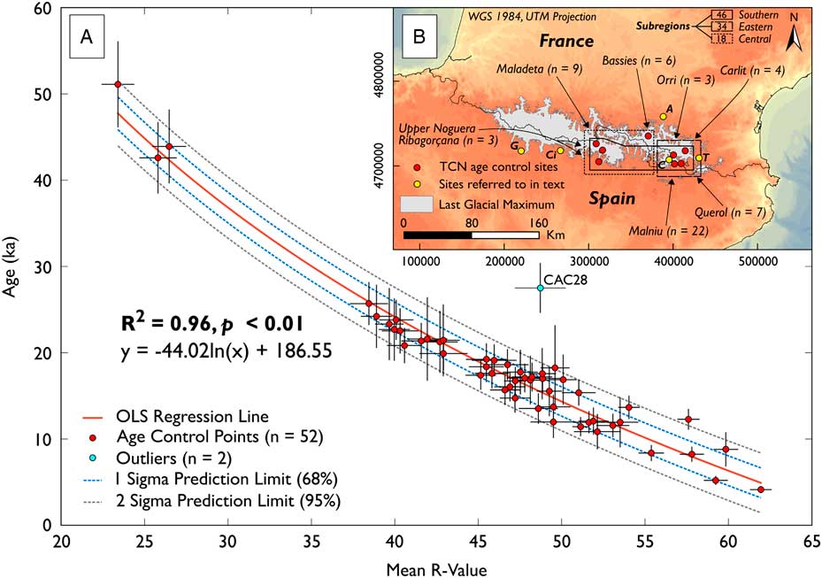
Figure 1 (colour online) Schmidt hammer exposure dating calibration curve for the Pyrenees. (A) Correlation between Schmidt hammer R values and terrestrial cosmogenic nuclide (TCN) exposure ages (n=53). Inherited outlier ICM04 not shown as it is beyond the graph axis (age=80.7±7.9 ka, R value=24.98±1.17). (B) Map of age control sites, sites referred to in text (A, Ariege; C, Campcardós; Ci, Cinca; G, Gállego; T, Têt), and the last glacial maximum extent after Calvet et al. (Reference Calvet, Delmas, Gunnell and Bourle2011).
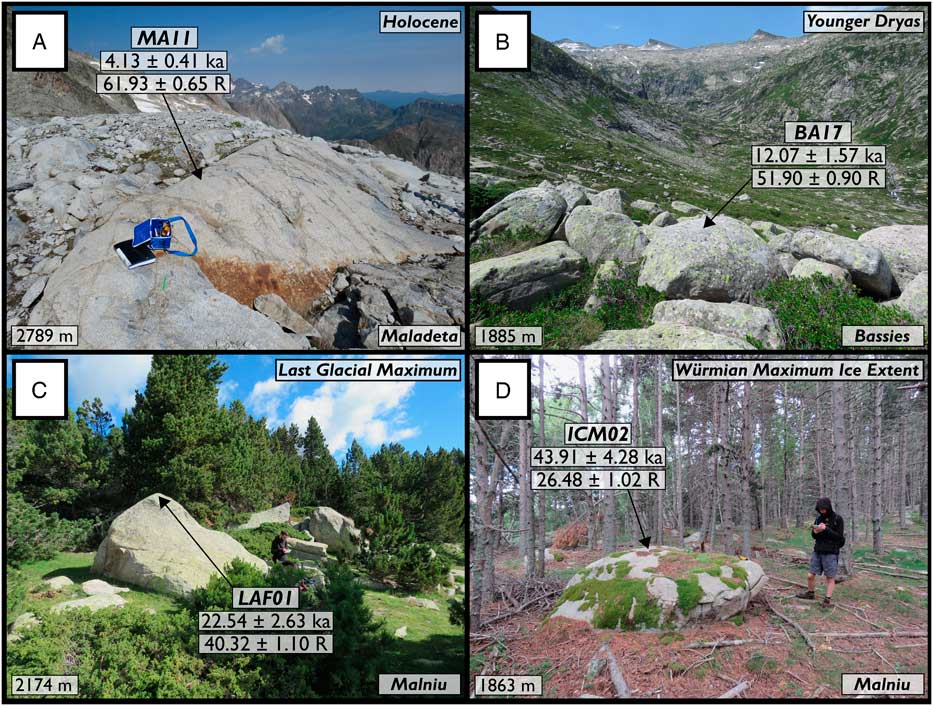
Figure 2 (colour online) 10Be-dated surfaces sampled using the Schmidt hammer. Holocene (A), Younger Dryas (B), last glacial maximum (C), and Würmian maximum ice extent (D) dated surfaces from Pallàs et al. (Reference Pallàs, Rodés, Braucher, Bourlès, Delmas, Calvet and Gunnell2010) and Crest et al. (Reference Crest, Delmas, Braucher, Gunnell and Calvet2017). Reported 10Be ages were recalibrated using the online calculators formerly known as the CRONUS-Earth online calculators (Balco et al., Reference Balco, Stone, Lifton and Dunai2008). Reported R values are the arithmetic mean of 30 R values (excluding no outliers)±the standard error of the mean.
Table 1 Details of 10Be-dated surfaces sampled using the Schmidt hammer.

a With reference to WGS 1984 31 T.
b C, central; E, eastern; S, southern.
c SEM, standard error of the mean.
d Inherited surface.
10Be exposure ages were recalibrated using the online calculators formerly known as the CRONUS-Earth online calculators (http://hess.ess.washington.edu/math/, accessed September 14, 2017, wrapper script 2.3, main calculator 2.1, constants 2.3, muons 1.1; Balco et al., Reference Balco, Stone, Lifton and Dunai2008). Exposure ages are based on the primary calibration data set of Borchers et al. (Reference Borchers, Marrero, Balco, Caffee, Goehring, Lifton, Nishiizumi, Phillips, Schaefer and Stone2016), the time-dependent Lm scaling (Lal, Reference Lal1991; Stone, Reference Stone2000), and assuming 0 mm/ka erosion. This approach is suitable as erosion rates for most glaciated crystalline rock surfaces are usually low (0.1–0.3 mm/ka; André, Reference André2002). Recalibrated ages must be treated as “minimum” ages because of the potential impact of surface erosion or transient shielding by snow or sediment cover. Two 10Be ages are likely compromised by prior exposure (inheritance) and are excluded from further analysis. Sample CAC28 from the Cometa d’Espagne cirque (26.96±2.89 ka; Crest et al., Reference Crest, Delmas, Braucher, Gunnell and Calvet2017) is proximal (~2 m) to three tightly clustered bedrock ages (CAC25=10.85±2.04 ka; CAC26=11.97±1.86 ka; CAC27=11.95±2.92 ka; mean squared weighted deviation [MSWD]=0.094). Similarly, sample ICM04 from the Malniu catchment (age=80.73±7.92 ka; Pallàs et al., Reference Pallàs, Rodés, Braucher, Bourlès, Delmas, Calvet and Gunnell2010) is proximal (~10 m) to three dated moraine boulders (ICM01=51.12±4.84 ka; ICM02=43.91±4.28 ka; ICM03=42.59±4.15 ka; MSWD=0.945). Both of these data sets are internally consistent (MSWD <1; ICM01-03; CAC25-27), which suggests that prior exposure, rather than post-depositional exhumation, accounts for the positively skewed distribution of 10Be ages. Remaining data (n=52) are used to construct an ordinary least squares regression from which numerical ages can be interpolated based on SH R values.
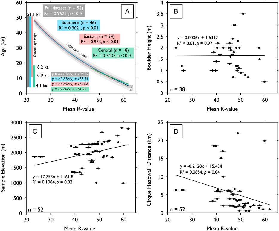
To test for regional variation in rates of subaerial weathering, age control data (n=52) were separated into subregions (Fig. 3A; southern, n=46; eastern, n=34; central, n=18). These data sets were used to construct logarithmic regressions for each subregion. For each subregion regression, ages were calculated at R value intervals of 0.1 over the associated calibration period (southern=4.1–51.1 ka; eastern=10.9–51.1 ka; central=4.1–18.2 ka). Interpolated ages were compared with the ages generated by the full age control data set, with two-sample Student’s t-tests used to evaluate whether the difference between subregion and full data set results was statistically significant. Subregion information is presented in Table 2.

Figure 3 Local and regional controls on surface R values. (A) Full data set (black) and subregion calibration curves for the southern (blue), eastern (red), and central Pyrenees (green). Subregion calibration curves fall within 1σ (dark grey) and 2σ (light grey) prediction limits of the full data set curve and imply no significant variation in the rate of rock surface weathering between subregions. (B) Boulder height (m) and surface R values (n=38). (C) Sample elevation (m) and surface R values (n=52). (D) Cirque headwall distance (km) and surface R values (n=52). These data (panels A–D) imply that site-specific factors have a negligible impact on subaerial weathering of granite surfaces in the central and eastern Pyrenees. (For interpretation of the references to colour in this figure legend, the reader is referred to the web version of this article.)
Table 2 Analysis of subregion data sets and comparison with the full age control data set (n=52).
These data imply little variation in the rate of subaerial weathering between subregions.
a Ages interpolated at R-value interval of 0.1 within these ranges.
b Mean variation from full data set ± mean absolute deviation.
c Mean calibration curve uncertainty of the full data set ± mean absolute deviation over the associated calibration period.
d P value of two-sample Student’s t-tests assuming unequal variance.
e H1, the difference between the two populations is statistically significant at P=0.05; H0, the difference between the two populations is not statistically significant at P=0.05.
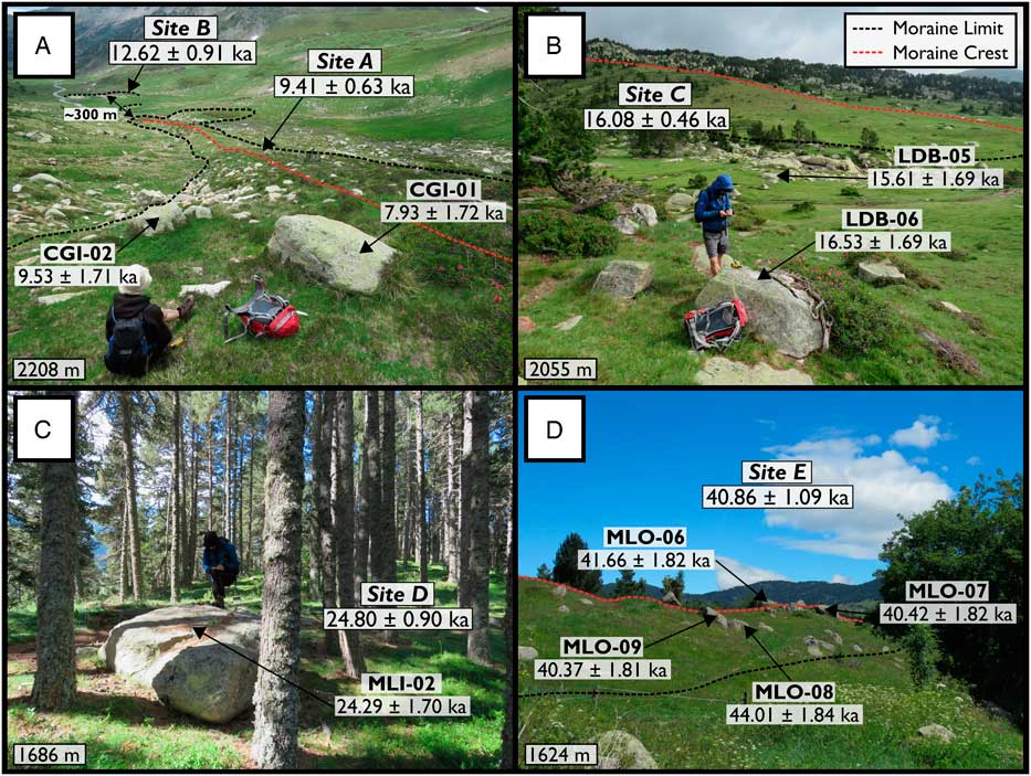
To verify the suitability of this TCN-SH calibration curve, 100 granite surfaces were sampled from five ice-front positions along an ~18 km transect of the Têt catchment, eastern Pyrenees (Fig. 4), with results validated against independent 10Be and 14C ages (Delmas et al., Reference Delmas, Gunnell, Braucher, Calvet and Bourlès2008)—that is, 10Be ages that do not comprise one of the 52 age control surfaces that underpin the calibration curve (Fig. 1). Of the 26 10Be ages reported by Delmas et al. (Reference Delmas, Gunnell, Braucher, Calvet and Bourlès2008), many postdate the timing of final deglaciation, likely because of moraine stabilisation processes (Hallet and Putknonen, Reference Gunnell, Calvet, Brichau, Carter, Aguilar and Zeyen1994). Despite this limitation, these data, in addition to geomorphological mapping of moraine stages (Fig. 5), provide a useful chronological framework for ice recession in the Têt catchment and can be used as independent evidence to verify the results of SHED. Sampled sites include proximal inner (site A, 1 km from catchment headwall, ~2200 m) and outer cirque moraines (site B, 1.3 km, ~2168 m). Based on existing 10Be ages, these moraines may reflect ice margin oscillations during the YD or early Holocene, although considerable age scatter (n=5; 12.00–13.99 ka) prevents accurate separation of glacial stages. Downvalley from these sites, glacially deposited boulders adjacent to a prominent lateral moraine (site C, 5.5 km, ~2051 m) are indicative of a post-LGM readvance of Têt glacier. This site is downvalley of the Grave-amont core site, which has produced 14C ages in the range 19.47–20.26 ka cal BP (n=3). These data suggest that Têt glacier was confined to the cirque environment as early as ~20 ka. Farther south, a large terminal moraine (site D, 18.5 km, ~1686 m), dated to 24.22±4.58 ka (n=1), likely marks the LGM ice extent. 10Be ages from this glacial stage exhibit considerable scatter (n=6; 15.6–24.2 ka) and likely reflect post-depositional exhumation of moraine boulders (Hallet and Putkonen, Reference Hallet and Putkonen1994). As a result, the precise age of this landform is unclear, which limits our understanding of the dynamics of Têt glacier during the global LGM. Finally, ~300 m outside of the LGM limit, the two outermost moraines of Têt glacier (site E, 18.8 km, ~1624 m) mark the Würmian MIE, although the precise age of this landform is unclear. These moraines record the maximum extent of glaciation in the Têt catchment, as the downstream landscape is dominated by fluvial incision. These moraines are morphologically distinct from proximal LGM moraines (Delmas et al., Reference Delmas, Gunnell, Braucher, Calvet and Bourlès2008), but it is not currently clear whether these landforms were deposited synchronously, with the outer moraines subject to intense moraine stabilisation processes since the LGM, or instead, whether the outer moraines represent an earlier glacial stage (MIS 3–4; Calvet et al., Reference Calvet, Delmas, Gunnell and Bourle2011). At each site, 20 surfaces were sampled for SHED following the methods described previously, with SH exposure ages and 1σ uncertainties calculated using SHED-Earth (http://shed.earth/, accessed September 15, 2017; Tomkins et al., Reference Tomkins, Huck, Dortch, Hughes, Kirkbride and Barr2018). To account for geologic uncertainty, which typically displays as positive and negative skew of data sets, probability density estimates (PDEs) were produced and modelled to separate out the highest probability Gaussian distribution (Fig. 5) as per the methods of Dortch et al. (Reference Dortch, Owen and Caffee2013). Using the KS density kernel in MATLAB (2015) and a dynamic smoothing window based on age uncertainty, PDE peaks and tails were separated into individual Gaussian distributions, the sum of which integrates to the cumulative PDE at 1000 iterations to obtain the best fit. The reintegrated PDE (made from the isolated Gaussians) goodness of fit is indicated graphically (Dortch et al., Reference Dortch, Owen and Caffee2013). Full sample information for the 100 surfaces sampled in the Têt catchment can be found in the Supplementary Materials.

Figure 4 (colour online) Sampled sites for Schmidt hammer exposure dating (SHED) from the Têt catchment, eastern Pyrenees. (A) Holocene (site A; 9.41±0.62 ka) and Younger Dryas moraines (site B; 12.62±0.91 ka). (B) The prominent lateral moraine and proximal surfaces sampled for SHED (site C; 16.08±0.46 ka). (C) Sampled surface from the large terminal moraine, previously dated to 24.22±4.58 ka (10Be, n=1; Delmas et al., Reference Delmas, Gunnell, Braucher, Calvet and Bourlès2008), which marks the maximum extent of ice during the last glacial maximum (site D; 24.80±0.90 ka). (D) The outermost moraine of Têt glacier and the Würmian maximum ice extent for this catchment (site E; 40.86±1.09 ka).
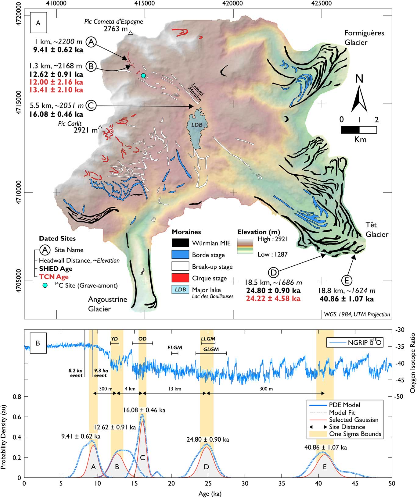
Figure 5 (colour online) A deglacial chronology for the Têt catchment, eastern Pyrenees. (A) Geomorphological map showing the Würmian maximum ice extent (MIE) for Têt, Angoustrine, and Formiguères glaciers. Moraine stages modified and terrestrial cosmogenic nuclide (TCN) exposure ages recalibrated from Delmas et al. (Reference Delmas, Gunnell, Braucher, Calvet and Bourlès2008). Schmidt hammer sampled sites (Circles A–E) are shown. (B) Probability density estimates (PDEs) and Gaussian models for sampled sites. (Plots A–E) are plotted against the North Greenland Ice Core Project (NGRIP) δ18O curve (Rasmussen et al., Reference Rasmussen, Bigler, Blockley, Blunier, Buchardt, Clausen and Cvijanovic2014). Key events are shown: Younger Dryas (YD), Oldest Dryas (OD), global last glacial maximum (GLGM), local last glacial maximum (LLGM), and the Eurasian last glacial maximum (ELGM).
RESULTS
A clear correlation between TCN exposure ages and SH R values is expressed by a logarithmic regression (Fig. 1A; n=52, R 2=0.96, P=<0.01). Boulder height (Fig. 3B; n=38; R 2=<0.01; P=0.97), sample elevation (Fig. 3C; R 2=0.11; P=0.02), and cirque headwall distance (Fig. 3D; R 2=0.09; P=0.04) have a negligible correlation with R values. Significant differences in R values between recently exposed surfaces (<5 ka; R values >60) and those exposed during the YD (R values ~50), the LGM (R values ~40), and the Würmian MIE (R values ≤30) indicate that age-related information can be retained with carborundum treatment (Moses et al., Reference Moses, Robinson and Barlow2014). There is no significant variation in subaerial weathering rate between subregions (Table 2, Fig. 3A) as eastern (n=34), central (n=18) and southern (n=46) curves are completely enclosed by the 1σ boundaries of the full data set curve and generate SH ages that vary from the full data set by ≤0.37 ka, ≤0.93 ka, and ≤0.22 ka, respectively. In addition, the average subregion variation from the full data set is limited to 0.11±0.06 ka and 0.14±0.08 ka for the southern and eastern data sets, respectively, increasing to 0.43±0.22 ka for the central data set. This likely reflects the limited calibration period (4.1–18.2 ka) and low number of age control surfaces (n=18) for the central data set. As a result, TCN-SH calibration curves should be based on large age control data sets (≥25 10Be ages; Tomkins et al., Reference Tomkins, Dortch and Hughes2016, Reference Tomkins, Huck, Dortch, Hughes, Kirkbride and Barr2018) to minimise the effect of individual exposure age errors. Despite this, two-sample Student’s t-tests indicate that variation between age estimates derived from the full data set and southern, eastern, and central data sets is not statistically significant (Table 2; P values >0.91).
In the Têt catchment, SH sampling of undated glacially deposited boulders reveals statistically significant differences (two-sample Student’s t-tests, P<0.01) between the mean SH R values of sequential glacial landforms (A-B, B-C, C-D, D-E). Statistically significant differences in mean SH R values are evident between both proximal (~300 m; A-B; D-E) and distal landforms (~13 km; C-D). These data were converted into numerical ages based on the TCN-SH calibration curve presented in this article (y=44.02ln(x) + 186.55), although these must be considered minimum ages as post-depositional erosion is assumed to be negligible (0 mm/ka). Incorporating an erosion rate of 0.3 mm/ka (André, Reference André2002) increases calibration 10Be ages (n=52) by ≤1.43% and by an average of ~0.64%, equivalent to ~0.7 ka for sample ICM01 (~50 ka) and ≤0.16 ka for surfaces exposed within the last ~25 ka. This variation is within measurement uncertainty for 10Be ages and is significantly less than the 1σ uncertainty of individual SH exposure ages (minimum=1.69 ka; maximum=1.85 ka). As a result, incorporating erosion has a negligible impact on calculated SH exposure ages, even for landforms deposited prior to the LGM. To account for geologic uncertainty in interpolated ages, PDE modelling (Dortch et al., Reference Dortch, Owen and Caffee2013) produces peak Gaussian distributions for glacial landforms in the Têt catchment of 9.41±0.62 ka (A), 12.62±0.91 ka (B), 16.08±0.46 ka (C), 24.80±0.90 ka (D), and 40.86±1.09 ka (E).
DISCUSSION
First, a strong correlation between 10Be ages and SH R values indicates that the primary control on surface R values is cumulative exposure to subaerial weathering (Tomkins et al., Reference Tomkins, Dortch and Hughes2016, Reference Tomkins, Huck, Dortch, Hughes, Kirkbride and Barr2018). This correlation is observed despite marked variability in sample elevations (elevation range=~1836 m), boulder heights (height=~0.5 to ~3.5 m), cirque headwall distances (~0.6 to ~22 km), and relative positions along the axis of the Pyrenean mountain range (Fig. 1B; maximum distance between samples=~110 km). These data match previous evidence from the British Isles (Tomkins et al., Reference Tomkins, Dortch and Hughes2016, Reference Tomkins, Huck, Dortch, Hughes, Kirkbride and Barr2018) and the Krkonoše Mountains, Poland/Czech Republic (Engel, Reference Engel2007; Engel et al., Reference Engel, Traczyk, Braucher, Woronko and Kŕížek2011), for a relationship between 10Be ages and subaerial weathering of granite surfaces. However, clear differences in effective calibration time scales in the British Isles (~25 ka), the Krkonoše Mountains (~15 ka), and the Pyrenees (~50 ka) indicate that weathering rates vary significantly between these regions, likely as a function of latitudinal gradients in either precipitation or temperature. The data presented in this study also provide further evidence that weathering rates are not linear but decrease over time (White and Brantley, Reference White and Brantley2003; Stahl et al., Reference Stahl, Winkler, Quigley, Bebbington, Duffy and Duke2013). For surfaces exposed prior to the LGM, slower rates of weathering likely reflect the formation of stable weathering residues, which slow water transport to unaltered material and impede chemical transport away from it (Colman, Reference Colman1981). Finally, these data imply little variation in the rate of rock surface weathering between subregions over the last ~50 ka (Table 2, Fig. 3A). It must be noted that this interpretation is based on the assumption that recalibrated 10Be ages are accurate ages for deglaciation, with no post-depositional erosion. If this assumption is not valid, then variable regional weathering rates could influence 10Be ages and introduce bias to the SHED calibration curve as distal surfaces exposed synchronously could return contrasting 10Be ages. However, under the assumption of minimal weathering of crystalline rock surfaces (0–3 mm/ka; André, Reference André2002), post-depositional erosion is unlikely to have significant impact on the results of SHED as differences in 10Be ages because of erosion are significantly smaller than 10Be measurement uncertainty (sample ICM01; 10Be age uncertainty=± 4.99 ka; age difference 0–3 mm/ka erosion=~0.7 ka). This appears to contrast with recent evidence from New Zealand, with marked local variability in rates of rock surface weathering (Stahl et al., Reference Stahl, Winkler, Quigley, Bebbington, Duffy and Duke2013). This variability necessitates local calibration curves for proximal sites (~100 km distance), which are applicable over contrasting calibration time scales (Saxton and Charwell River terraces=~10 ka; Waipara River terraces=~1 ka; cf. Fig. 2 in Stahl et al., Reference Stahl, Winkler, Quigley, Bebbington, Duffy and Duke2013). New data from the Pyrenees indicate that subaerial weathering of granite surfaces is consistent across the central and eastern Pyrenees, which implies that equivalent time-dependent weathering of granite surfaces can occur over significant spatial scales for regions of similar climate (Tomkins et al., Reference Tomkins, Dortch and Hughes2016, Reference Tomkins, Huck, Dortch, Hughes, Kirkbride and Barr2018).
In the Têt catchment, age estimates derived from PDE modelling of Gaussian distributions (Dortch et al., Reference Dortch, Owen and Caffee2013) are in correct stratigraphic order, are consistent with existing interpretations of post-MIE glaciation (Fig. 5), and are supported by independent 10Be ages, which provide a chronological framework for the retreat dynamics of Têt glacier during the Würmian (Delmas et al., Reference Delmas, Gunnell, Braucher, Calvet and Bourlès2008). Gaussian ages clearly differentiate LGM (D: 24.80±0.90 ka) and Würmian MIE (E: 40.86±1.09 ka) glacial deposits and provide firm evidence of comparable glacier lengths during MIS 2 and MIS 3 (~300 m difference). This contrasts markedly with evidence from the western Pyrenees, where glaciers failed to reach MIE limits during the LGM (≥15 km difference; Gállego catchment; Jalut et al., Reference Jalut, Monserrat Marti, Fontugne, Delibrias, Vilaplana and Julia1992; Calvet et al., Reference Calvet, Delmas, Gunnell and Bourle2011). The proximity of MIE and LGM deposits matches the geomorphological record in Malniu (~330 m) and Querol (~600 m) and indicates that glaciers in the eastern Pyrenees advanced significantly during MIS 2 to near MIE limits, irrespective of glacier size (Querol: ~25 km; Têt: ~18.5 km; Malniu: ~6 km). A MIS 3 Würmian MIE (40.86±1.09 ka) matches ages from a terminal moraine in Malniu (TCN; n=3; 42.6–51.1 ka; Pallàs et al., Reference Pallàs, Rodés, Braucher, Bourlès, Delmas, Calvet and Gunnell2010), a midvalley lateral moraine in the Ariege (TCN; n=1; 37.89±9.98 ka; Delmas et al., Reference Delmas, Calvet, Gunnell, Braucher and Bourlès2011), and OSL ages from the Senegüe terminal moraine in the Gállego catchment (n=2; ~36 ka; Lewis et al., Reference Lewis, Mcdonald, Sancho, Peña and Rhodes2009). These data contrast with MIS 4 ages from ice-contact lake deposits in the Cinca catchment (OSL; n=3; 46–71 ka; Lewis et al., Reference Lewis, Mcdonald, Sancho, Peña and Rhodes2009) and from the terminal moraine in the Ariege catchment (TCN; n=1; 88.78±18.37 ka; Delmas et al., Reference Delmas, Calvet, Gunnell, Braucher and Bourlès2011). Regardless of the precise timing of the MIE, one of the most valuable contributions of SHED is its ability to differentiate proximal LGM and MIE glacial deposits and thus enable robust comparison of glacier length fluctuations across the Pyrenees.
By comparison, the timing of the local MIS 2 glacial maximum in the Têt catchment is constrained by both TCN (n=1; 24.22±4.58 ka) and SHED ages (n=13; 24.80±0.90 ka). These data accord with recent evidence that ice masses in the European Alps reached their maximum extents at 24–26 ka because of the growth of the Laurentide Ice Sheet, which reached its maximum close to this time (>23.0±0.6 ka; Ullman et al., Reference Ullman, Carlson, LeGrande, Anslow, Moore, Caffee, Syverson and Licciardi2015), and the southward advection of the polar front (Monegato et al., Reference Monegato, Scardia, Hajdas, Rizzini and Piccin2017). These events coincided with reduced solar radiation towards the solar minimum in the Northern Hemisphere at ~24 ka (Alley et al., Reference Alley, Brook and Anandakrishnan2002). In addition to SHED and TCN ages from the Têt catchment, an Alpine LGM is supported by post-maximum TCN ages from Querol (YRA samples; n=3; 22.7–24.2 ka), the oldest ages from the frontal lobe (OEC01; 23.8±2.3 ka) and a coeval lateral moraine (LAF04; 25.7±2.7 ka) in Malniu (Pallàs et al., Reference Pallàs, Rodés, Braucher, Bourlès, Delmas, Calvet and Gunnell2010), and 14C ages from the Gállego catchment, which indicate that the MIS 2 MIE occurred by 24.21 ka cal BP (Jalut et al., Reference Jalut, Monserrat Marti, Fontugne, Delibrias, Vilaplana and Julia1992). The asynchroneity of Alpine glaciers and the Eurasian ice sheets at the global LGM, the latter reaching its maximum extent at ~21 ka (Hughes et al., Reference Hughes, Gyllencreutz, Lohne, Mangerud and Svendsen2016), demonstrates the sensitivity of Alpine ice masses to the advection of moisture from the Mediterranean Sea (Luetscher et al., Reference Luetscher, Boch, Sodemann, Spötl, Cheng, Edwards, Frisia, Hof and Müller2015). The contrasting size of Pyrenean glaciers at the LGM likely reflects the relative influence of weather systems from the Atlantic and the western Mediterranean, the latter favouring cyclogenesis, convection of moist air, and increased precipitation to coastal mountain ranges (Kuhlemann et al., Reference Kuhlemann, Rohling, Krumrei, Kubik, Ivy-Ochs and Kucera2008). However, this hypothesis is tentative owing to limited geochronological data for MIS 2 glaciers in the western Pyrenees. SHED is a viable method to address this knowledge gap as the calibration curve is well constrained by age control points that span the global LGM and is able to reproduce the LGM TCN age in the Têt catchment, varying by <0.6 ka.
Finally, the geomorphological record indicates that post-LGM retreat was dynamic (Fig. 5; Borde and Cirque Stages). A number of readvance events are captured by SHED, with moraines deposited during the Oldest Dryas (OD; C: 16.08±0.46 ka), YD (B: 12.62±0.91 ka), and early Holocene (A: 9.41±0.62 ka). Evidence for a significant readvance during the OD is matched by TCN ages from the Orri (CPM; n=3; 16.41±0.58 ka) and Malniu catchments (IMA; n=5; 16.68±0.52 ka) and is consistent with evidence for major advances in the western Pyrenees (Palacios et al., Reference Palacios, García-Ruiz, Andrés, Schimmelpfennig, Campos and Léanni2017). However, these data conflict markedly with 14C ages from the Grave-amont core site (Fig. 5; 19.47–20.26 ka cal BP), which indicate rapid post-LGM retreat (~3.3 km/ka). New SHED data indicate that this deposit must have been overridden (Delmas et al., Reference Delmas, Gunnell, Braucher, Calvet and Bourlès2008; Crest et al., Reference Crest, Delmas, Braucher, Gunnell and Calvet2017). In addition, SHED clearly differentiates proximal (~300 m) YD (B: 12.62±0.91 ka) and Holocene (A: 9.41±0.62 ka) moraines. TCN exposure ages from the YD moraine (sample N; 12.0±2.2 ka) and proximal bedrock surfaces (sample O2; 13.4±2.1 ka) give contrasting age estimates but are broadly consistent with the SHED estimate. The age of the inner cirque moraine (A) overlaps with the 9.3 ka event (Rasmussen et al., Reference Rasmussen, Bigler, Blockley, Blunier, Buchardt, Clausen and Cvijanovic2014), although complete deglaciation and readvance of ice in the Têt catchment after the YD seems unlikely owing to the short time frame of this cooling event (~110 yr). Instead, this moraine likely marks a stillstand or readvance of the ice margin from sheltered cirques below Pic Cometa d’Espagne. These data in their totality indicate that cirque (A-B) and valley moraines (C) reflect stillstands or readvances of Têt glacier, potentially in response to North Atlantic climate fluctuations (OD, YD, 9.3 ka event). These glacial deposits provide a valuable record of ice margin fluctuations, and yet the post-LGM history of the Pyrenean ice field is currently poorly understood (Calvet et al., Reference Calvet, Delmas, Gunnell and Bourle2011). Future research using SHED must seek to accurately differentiate post-LGM ice masses to provide robust information on the response of these glaciers to North Atlantic climate variability.
This new SHED calibration curve demonstrates that this method can be applied successfully in contrasting climatic regimes and that equivalent time-dependent weathering of granite surfaces can occur within regions of similar climate (Tomkins et al., Reference Tomkins, Dortch and Hughes2016, Reference Tomkins, Huck, Dortch, Hughes, Kirkbride and Barr2018). TCN-SH calibration curves based on significant age control data sets (n ≥ 50) have been shown to produce robust ages for glacial landforms, as demonstrated through comparison with independent radiometric ages (10Be), and in aggregate, can generate results of comparable accuracy and precision to TCN dating. This approach could be replicated in similar well-dated granite regions throughout the world (e.g., Himalaya, Patagonia, and Sierra Nevada) and has the ability to revolutionise high-sample, low-budget quantitative studies in Quaternary science. In the Pyrenees, future applications of SHED are needed to (1) separate LGM and Würmian MIE landforms across the mountain range and (2) address gaps in our understanding of post-LGM retreat (Calvet et al., Reference Calvet, Delmas, Gunnell and Bourle2011). The relative scarcity of geochronological data, particularly in the western Pyrenees, has thus far prevented a Pyrenean-scale synthesis of post–MIS 4 glaciation, although progress continues to be made (e.g., Palacios et al., Reference Palacios, García-Ruiz, Andrés, Schimmelpfennig, Campos and Léanni2017). Widespread application of SHED across the Pyrenees would generate a wealth of new chronological data related to glacier oscillations over the last ~50 ka and would likely accelerate progress in our understanding of the last Pleistocene glacial cycle.
To apply this regional calibration curve to undated landforms or to verify its accuracy on landforms dated using radiometric methods (TCN, OSL, 14C), users should follow the methods described previously and perform (1) instrument calibration and (2) age calibration procedures as described fully in Tomkins et al. (Reference Tomkins, Huck, Dortch, Hughes, Kirkbride and Barr2018). To perform instrument calibration, users should sample a suitable surface before and after data collection that returns R values that lie within the range of R values measured in the field (Tomkins et al., Reference Tomkins, Huck, Dortch, Hughes, Kirkbride and Barr2018). In contrast, instrument calibration using the test anvil (R value=81±2; Proceq, 2004) is inappropriate for surfaces typically tested by Quaternary researchers (R values: 25–60) and should only be utilised for the hardest natural rock surfaces (R values ≥70). To perform age calibration and to standardise different SHs and different user strategies to the Pyrenean calibration curve, users should test their SH on one of three calibration surfaces provided (mean of 30 R values; Table 3; sample photos available at http://shed.earth) rather than the University of Manchester calibration boulder as described in Dortch et al. (Reference Dortch, Hughes and Tomkins2016). Users should compare the recorded mean R value against the assigned value (Table 3) to calculate a correction factor, which is then applied to all user data. This functionality is incorporated into SHED-Earth. These procedures facilitate comparison between studies and encourage wider and more consistent application of SHED throughout the Pyrenees.
Table 3 Age calibration surfaces for the Pyrenees.

Detailed information on age calibration can be found in Tomkins et al. (Reference Tomkins, Huck, Dortch, Hughes, Kirkbride and Barr2018) or at http://shed.earth. Users should test their Schmidt hammer on one of these calibration surfaces provided (mean of 30 R values) and input their results into the SHED-Earth online calculator. Age calibration standardizes different Schmidt hammers and user strategies to the regional calibration curve.
a With reference to WGS 1984 31 T.
b SEM, standard error of the mean.
CONCLUSIONS
Quaternary deposits in the Pyrenees are ideally placed for paleoclimate studies given their proximity to both the North Atlantic and the Mediterranean. However, limited geochronological data sets, the increasing fragmentation of trunk glaciers, and the incomplete nature of the geomorphological record have prevented a regional-scale synthesis of post–MIS 4 glaciation. The Pyrenees are ideally suited for SHED given the excellent preservation of glacial deposits and the abundance of granite glacial boulders and erosion surfaces.
In this study, we show that SHED is a viable geochronological technique, as a strong correlation between 52 TCN exposure ages and SH R values (R 2=0.96, P<0.01) permits the use of the SH as a numerical dating tool. The effectiveness of this method is demonstrated for the Têt catchment in the eastern Pyrenees, where SH exposure ages are in correct stratigraphic order, are consistent with existing geomorphological interpretations, and show excellent agreement with previous TCN ages. SHED data confirm comparable glacier lengths during the LGM and the MIE in the eastern Pyrenees (~300 m), in contrast to evidence from the western Pyrenees (>15 km), and also confirm the antiquity of the MIE, which likely occurred during MIS 3 (40.86±1.09 ka). Moreover, SHED data show that glaciers in the eastern Pyrenees reached their maximum extents during the global LGM, synchronous with Alpine ice masses (24–26 ka). Glacier expansion was driven by enhanced moisture availability caused by southward advection of the polar front coinciding with the maximum extent of the Laurentide Ice Sheet and a solar minimum at ~24 ka.
SHED is cost and time efficient and can differentiate proximal glacial deposits (~300 m), and in aggregate, can generate results of comparable accuracy and precision to TCN dating. Moreover, our approach provides new evidence for non-linear weathering of granitic surfaces through time, likely associated with the formation of stable weathering residues. Finally, our data imply little variation in the rate of subaerial weathering between subregions over the last ~50 ka, which indicates that our calibration curve can be applied widely throughout the central and eastern Pyrenees.
ACKNOWLEDGMENTS
This project was supported by the Royal Geographical Society (with the Institute of British Geographers) with a Dudley Stamp Memorial Award and by the University of Manchester SEED Fieldwork Support Fund. MT is a recipient of a University of Manchester President’s Doctoral Scholar Award and this research forms part of his PhD. JMD, PDH, and JJH would like to thank the University of Manchester Research Stimulation Fund. We would also like to thank Prof. John Matthews, associate editor Prof. James Shulmeister, and an anonymous reviewer for their constructive reviews.
SUPPLEMENTARY MATERIAL
To view supplementary material for this article, please visit https://doi.org/10.1017/qua.2018.12