


INTRODUCTION
Resolving temporal questions at decadal or annual scales using radiocarbon (14C) dates is difficult (Bronk Ramsey, Reference Bronk Ramsey2008). This is especially true of cases in which researchers attempt to distinguish a synchronous event from an asynchronous process that occurred over multiple years or decades. Here, we consider two 14C datasets relevant to this problem: 14C measurements associated with the Laacher See volcanic eruption in Germany (Baales et al., Reference Baales, Jöris, Street, Bittmann, Weninger and Wiethold2002) and 14C measurements associated with the hypothesized Younger Dryas extraterrestrial impact, recovered from contexts in Asia, Europe, and North America (Fig. 1; Kennett et al., Reference Kennett, Kennett, Culleton, Aura Tortosa, Bischoff, Bunch and Daniel2015). In principle, calibrated 14C measurements of organic material associated with each event or hypothesized event should be tightly clustered around a value corresponding to the calendar year of that event. However, in practice, multiple sources of uncertainty may cause 14C measurements to be more dispersed than expected, obscuring the difference between a synchronous depositional event and a depositional process that occurred over multiple decades or centuries (Baillie, Reference Baillie1991).

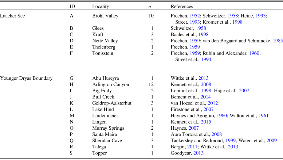
Figure 1. Map of Laacher See Tephra (LST) and Younger Dryas Boundary (YDB) localities. Inset map (green border) shows detailed view of localities in northern Europe. Alphabetic site IDs are listed in Table 1. (For interpretation of the references to color in this figure legend, the reader is referred to the web version of this article.)
Sources of uncertainty include imprecision in the measurement of 14C, captured in reported measurement errors, and in the calibration of those measurements into calendar years (Bronk Ramsey, Reference Bronk Ramsey2008). The 14C measurement and calibration process produces continuous non-normal, often multimodal, calendar date distributions with high probability regions that can span multiple centuries (Bronk Ramsey, Reference Bronk Ramsey2009a). Additional uncertainty can arise from chronological mismatches between the death and deposition of sample organisms, often referred to as “old wood” effects (Dean, Reference Dean1978; Schiffer, Reference Schiffer1986; Bronk Ramsey, Reference Bronk Ramsey2009b), as well as systematic biases in laboratory measurements and variability in measurement repeatability between laboratories (Polach, Reference Polach, Stanley and Scoggins1974; International Study Group, 1982; Scott et al., Reference Scott, Aitchison, Harkness, Cook and Baxter1990, Reference Scott, Harkness and Cook1998, Reference Scott, Cook, Naysmith, Bryant and O'Donnell2007, Reference Scott, Cook and Naysmith2010a, Reference Scott, Cook and Naysmith2010b Boaretto et al., Reference Boaretto, Bryant, Carmi, Cook, Gulliksen, Harkness, Heinemeier, McClure, McGee and Naysmith2003; Christen and Pérez, Reference Christen and Pérez2009). The direction and magnitude of these sources of uncertainty are not constant, varying from one set of 14C measurements to another.
Existing statistical methods for evaluating synchroneity in 14C datasets do not fully account for these context-dependent uncertainties. One such method applies a χ2 test to a series of 14C measurements under the null hypothesis that the 14C measurements are of the same calendar age (Ward and Wilson, Reference Ward and Wilson1978). However, when this approach is applied to complex synchronous 14C datasets with many sources of uncertainty, it can generate large χ2 test statistics with low P values, and so falsely reject synchroneity. A more recent approach to determining whether two dates could be synchronous involves calculating the distribution of temporal distances between both calibrated age densities (Parnell et al., Reference Parnell, Haslett, Allen, Buck and Huntley2008; see also, the Difference command in the Oxcal 14C calibration software [Bronk Ramsey, Reference Bronk Ramsey2008]). If the 95% highest density interval of this distribution includes zero (i.e., there is some overlap in the calibrated age densities at the 95% threshold), synchroneity is considered plausible and therefore not rejected. However, this approach cannot estimate the probability of obtaining the observed age densities, given a synchronous event, and thus does not distinguish between datasets that are unlikely to have been generated by a synchronous event and those that are more likely to have been deposited synchronously.
In this paper, we develop a simulation-based technique for assessing synchroneity that accounts for the sources of uncertainty specific to a given 14C dataset. We apply this technique to the observed 14C datasets associated with the Laacher See volcanic eruption and the hypothesized Younger Dryas extraterrestrial impact. Here, we define a “geologically synchronous event” as an event that deposited organic material within a one-year period.
Laacher See volcanic eruption and associated 14C dataset
The Laacher See (Germany) volcanic eruption occurred ~12,900 cal yr BP (Schmincke et al., Reference Schmincke, Park and Harms1999; Baales et al., Reference Baales, Jöris, Street, Bittmann, Weninger and Wiethold2002). The volcano, located in western Germany, ~40 km south of the city of Bonn, consists of two craters linked by a single submerged vent (van den Bogaard and Schmincke, Reference van den Bogaard and Schmincke1985; Baales et al., Reference Baales, Jöris, Street, Bittmann, Weninger and Wiethold2002). The Laacher See Tephra (LST) is concentrated in central Europe, with associated ash having been identified as far south as Italy, north to the Baltic Sea, west into France, and east into Poland (van den Bogaard and Schmincke, Reference van den Bogaard and Schmincke1985; Schmincke et al., Reference Schmincke, Park and Harms1999). The LST is visible in three geochemically distinct stratigraphic layers representing three eruptive phases: the Lower, Middle, and Upper LST. Combined, these three layers form a tephra that exceeds 50 m thick near the volcanic vent, decreasing to ~10 m thick at four km from the vent (Schmincke et al., Reference Schmincke, Park and Harms1999).
The bulk of volcanic activity likely occurred over a span of ~10 hours, with complete deposition of the three associated LST layers within a period of several months (Schmincke et al., Reference Schmincke, Park and Harms1999). Given that deposition of the combined Lower, Middle, and Upper LST occurred within a single calendar year (van den Bogaard, Reference van den Bogaard1983; van den Bogaard and Schmincke, Reference van den Bogaard and Schmincke1985; Park and Schmincke, Reference Park and Schmincke1997; Schmincke et al., Reference Schmincke, Park and Harms1999), the Laacher See volcanic eruption meets our definition for a geologically synchronous event. We thus treat 14C samples from any of the three layers as originating from the same event (sensu Baales et al., Reference Baales, Jöris, Street, Bittmann, Weninger and Wiethold2002).
We identified 19 previously published 14C measurements on samples collected from within the Lower, Middle, or Upper LST at six German localities (Fig. 2, Table 1). All but one measurement (HV-11774, short lived plant remains) are on wood samples, primarily trees of the genus Populus, and none of them are accelerator mass spectrometer (AMS) measurements. We excluded three LST 14C measurements from Kruft that correspond to three sequential sets of rings from one tree specimen, Populus 9 (measurements HD-19092, HD-18622, and HD-19037), and only included the measurement taken on the outermost available Populus 9 rings, HD-19098, corresponding to the 14C measurement for a date closest to the deposition of the LST. These 19 14C measurements constitute the observed LST dataset (LSTObs).

Figure 2. Calibrated age densities for samples originating from LST contexts (LSTObs). The right column of text displays the means and standard errors for each sample in 14C yr BP. Light blue distributions show dates obtained through gas proportional or liquid scintillation counting. Open densities correspond to dates with potential “old wood” effects (all samples other than HV-11774). The grey band marks the range of possible years for the Laacher See volcanic eruption, 12,966–12,866 cal yr BP. Question marks denote samples for which original sources did not report laboratory sample IDs. See Table 1 for references. (For interpretation of the references to color in this figure legend, the reader is referred to the web version of this article.)
Table 1. Laacher See Tephra and Younger Dryas Boundary localities with number (n) of 14C measurements. Alphabetic ID corresponds to site locations in Figure 1.
Previous research with 14C dates, lake varve records, and tree-ring chronologies suggests a most likely calendar date of 12,916 cal yr BP for the deposition of the LST (Baales et al., Reference Baales, Jöris, Street, Bittmann, Weninger and Wiethold2002). Given that the true date is imprecisely known, we consider a 101-yr window centered on this date (12,966 to 12,866 cal yr BP).
The Younger Dryas Boundary (YDB) and associated 14C dataset
The Younger Dryas Impact Hypothesis posits that an extraterrestrial body collided with North America, most likely on some date between 12,835 and 12,735 cal yr BP (Kennett et al., Reference Kennett, Kennett, Culleton, Aura Tortosa, Bischoff, Bunch and Daniel2015), causing widespread burning, megafaunal extinctions, the onset of Younger Dryas cooling, and the disappearance of the Clovis archaeological culture (Firestone et al., Reference Firestone, West, Kennett, Becker, Bunch, Revay and Schultz2007; Kennett et al., Reference Kennett, Kennett, West, Erlandson, Johnson, Hendy, West, Culleton, Jones and Staffordjr2008, Reference Kennett, Kennett, Culleton, Aura Tortosa, Bischoff, Bunch and Daniel2015; Firestone, Reference Firestone2009; Wolbach et al., Reference Wolbach, Ballard, Mayewski, Adedeji, Bunch, Firestone and French2018a, Reference Wolbach, Ballard, Mayewski, Parnell, Cahill, Adedeji and Bunch2018b). Supporters of the hypothesis argue that this event is recognizable in the Younger Dryas Boundary (YDB) stratum at sites in North and South America, Europe, and Asia based on the presence of impact proxies such as nanodiamonds, carbon spherules, magnetic spherules, and increased platinum (Firestone et al., Reference Firestone, West, Kennett, Becker, Bunch, Revay and Schultz2007; Kennett et al., Reference Kennett, Kennett, West, Erlandson, Johnson, Hendy, West, Culleton, Jones and Staffordjr2008, Reference Kennett, Kennett, West, Mercer, Hee, Bement, Bunch, Sellers and Wolbach2009a, Reference Kennett, Kennett, West, West, Bunch, Culleton, Erlandson, Hee, Johnson and Mercer2009b, Reference Kennett, Kennett, Culleton, Aura Tortosa, Bischoff, Bunch and Daniel2015; Firestone, Reference Firestone2009; Israde-Alcantara et al., Reference Israde-Alcantara, Bischoff, Dominguez-Vazquez, Li, DeCarli, Bunch and Wittke2012; Bunch et al., Reference Bunch, Hermes, Moore, Kennett, Weaver, Wittke and DeCarli2012; LeCompte et al., Reference LeCompte, Goodyear, Demitroff, Batchelor, Vogel, Mooney, Rock and Seidel2012; Petaev et al., Reference Petaev, Huang, Jacobsen and Zindler2013; Wittke et al., Reference Wittke, Weaver, Bunch, Kennett, Kennett, Moore and Hillman2013; Wu et al., Reference Wu, Sharma, LeCompte, Demitroff and Landis2013; Kinzie et al., Reference Kinzie, Que Hee, Stich, Tague, Mercer, Razink and Kennett2014; Moore et al., Reference Moore, West, LeCompte, Brooks, Daniel, Goodyear and Ferguson2017; Kletetschka et al., Reference Kletetschka, Vondrák, Hruba, Prochazka, Nabelek, Svitavská-Svobodová and Bobek2018; Pino et al., Reference Pino, Abarzúa, Astorga, Martel-Cea, Cossio-Montecinos, Navarro and Paz Lira2019). However, independent researchers have failed to identify the proposed impact proxies in YDB aged sediments (Surovell et al., Reference Surovell, Holliday, Gingerich, Ketron, Haynes, Hilman, Wagner, Johnson and Claeys2009; Daulton et al., Reference Daulton, Pinter and Scott2010, Reference Daulton, Amari, Scott, Hardiman, Pinter and Anderson2017; Haynes et al., Reference Haynes, Boerner, Domanik, Lauretta, Ballenger and Goreva2010; Holliday et al., Reference Holliday, Surovell and Johnson2016), questioned whether the markers are necessarily the result of an impact (van der Hammen and van Geel, Reference van der Hammen and van Geel2008; A.C. Scott et al., Reference Scott, Pinter, Collinson, Hardiman, Anderson, Brain, Smith, Marone and Stampanoni2010; Pigati et al., Reference Pigati, Latorre, Rech, Betancourt, Martinez and Budahn2012; van Hoesel et al., Reference van Hoesel, Hoek, Braadbaart, van der Plicht, Pennock and Drury2012), criticized the methodologies used to date layers containing impact markers (Holliday and Meltzer, Reference Holliday and Meltzer2010; Blaauw et al., Reference Blaauw, Holliday, Gill and Nicoll2012; Meltzer et al., Reference Meltzer, Holliday, Cannon and Miller2014; van Hoesel et al., Reference van Hoesel, Hoek, Pennock and Drury2014), or disputed the plausibility of an impact or airburst as described by proponents (Boslough et al., Reference Boslough, Nicoll, Holliday, Daulton, Meltzer, Pinter and Scott2012). Proponents have also recently proposed that the hypothesized event produced the Hiawatha impact crater located in Greenland (Pino et al., Reference Pino, Abarzúa, Astorga, Martel-Cea, Cossio-Montecinos, Navarro and Paz Lira2019). However, the age of this crater remains unknown, with constraints suggesting only that it was formed some time during the Pleistocene (~11,000–2,588,000 cal yr BP; Kjær et al., Reference Kjær, Larsen, Binder, Bjørk, Eisen, Fahnestock and Funder2018).
We collated measurements specified by Kennett et al. (Reference Kennett, Kennett, Culleton, Aura Tortosa, Bischoff, Bunch and Daniel2015) as originating from a YDB layer containing impact markers. Kennett et al. (Reference Kennett, Kennett, Culleton, Aura Tortosa, Bischoff, Bunch and Daniel2015) identified YDB layers at 23 sites in North and South America, Europe, and Asia. Earlier iterations of the Younger Dryas Impact Hypothesis included additional sites, such as Wally's Beach, Howard Bay, Myrtle Beach, and Lumberton (Firestone et al., Reference Firestone, West, Kennett, Becker, Bunch, Revay and Schultz2007; Firestone, Reference Firestone2009). However, other researchers were unable to confirm the presence of impact markers (Paquay et al., Reference Paquay, Goderis, Ravizza, Vanhaeck, Boyd, Surovell, Holliday, Haynes and Claeys2009) or questioned the age of these sites (Pinter et al., Reference Pinter, Scott, Daulton, Podoll, Koeberl, Anderson and Ishman2011; Meltzer et al., Reference Meltzer, Holliday, Cannon and Miller2014), and proponents of the hypothesis have since dropped them from consideration. Of the 23 sites presented in Kennett et al. (Reference Kennett, Kennett, Culleton, Aura Tortosa, Bischoff, Bunch and Daniel2015), 13 have 14C samples taken directly from the YDB. In total, Kennett et al. (Kennett et al., Reference Kennett, Kennett, Culleton, Aura Tortosa, Bischoff, Bunch and Daniel2015) identified 32 YDB 14C samples from these 13 sites.
We considered those 32 14C samples presented by Kennett et al. (Reference Kennett, Kennett, Culleton, Aura Tortosa, Bischoff, Bunch and Daniel2015) as originating from the YDB. However, we subsequently excluded two of these samples: AA-25778 from Big Eddy (10,260 ± 85 14C yr BP) and TX-1044 from Murray Springs (12,600 ± 2440 14C yr BP). We excluded AA-25778 since it was flagged as an outlier in Kennett et al.'s (Reference Kennett, Kennett, Culleton, Aura Tortosa, Bischoff, Bunch and Daniel2015) age-depth model and TX-1044 due to its anomalously large measurement error. This left 30 14C measurements in the observed YDB 14C dataset (YDBObs; ×Fig. 3, Table 1). All but three of the 30 14C measurements in YDBObs are AMS (A-1045, TX-1045, and I-141). Most of these measurements are charcoal samples (n = 17), although wood (n = 7), soil organic matter (SOM; n = 2), bone (n = 1), and carbon elongate/spherule (n = 3) samples are also present. As Kennett et al. (Reference Kennett, Kennett, Culleton, Aura Tortosa, Bischoff, Bunch and Daniel2015) proposed a likely calendar age for the hypothesized impact between 12,835 and 12,735 cal yr BP, we consider the 101 calendar yr in this range.
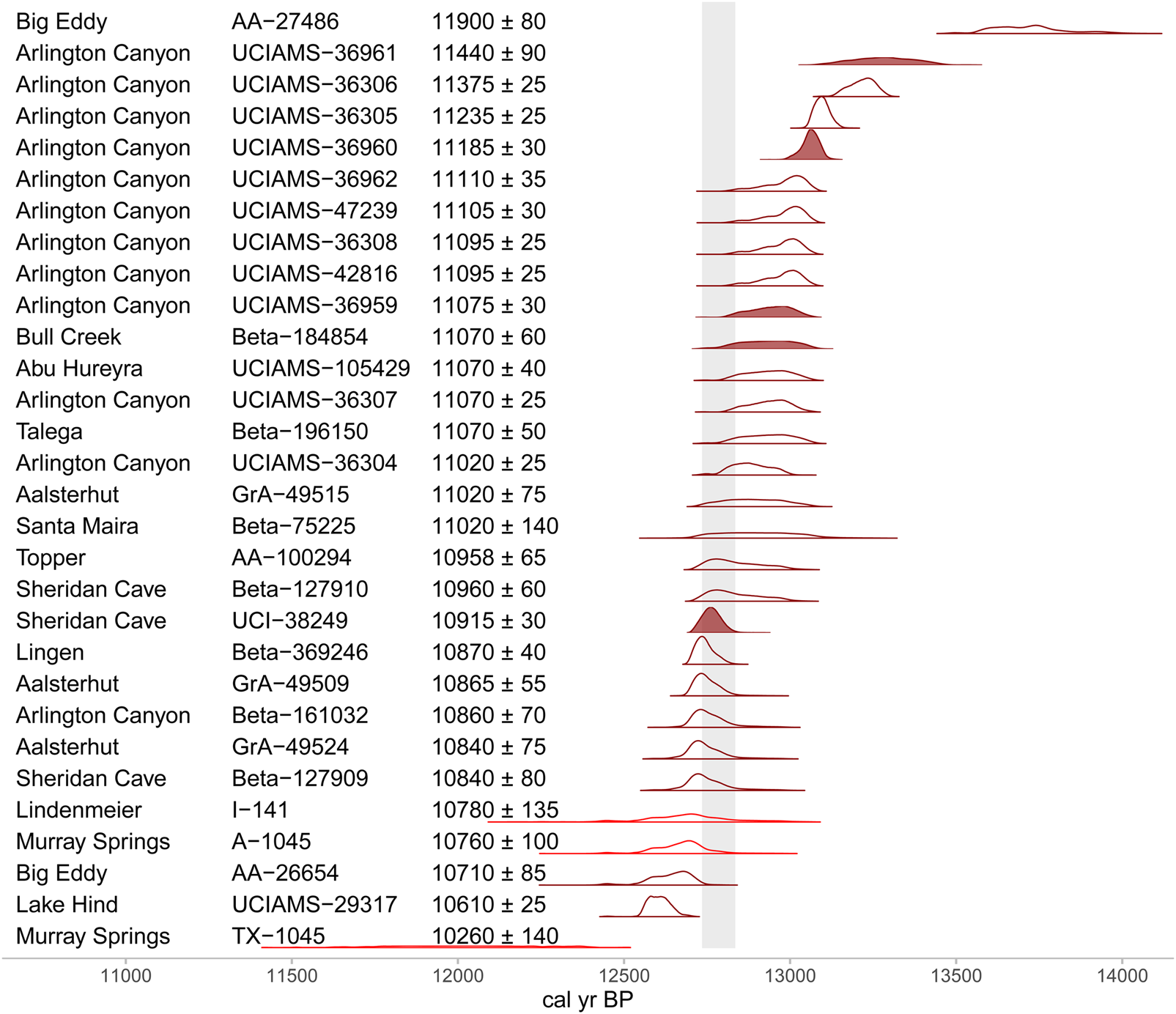
Figure 3. Calibrated age densities for samples originating from YDB contexts (YDBObs). The right column of text displays the means and standard errors for each sample in 14C yr BP. Dark red distributions show accelerator mass spectrometry (AMS) dates and light red distributions show dates obtained through gas proportional or liquid scintillation counting. Open densities correspond to dates with potential “old wood” effects. The grey band marks the range of possible years for the hypothesized extraterrestrial impact, 12,835–12,735 cal yr BP. See Table 1 for references. (For interpretation of the references to color in this figure legend, the reader is referred to the web version of this article.)
Supplementary data details the LSTObs and YDBObs14C samples, including additional 14C samples that we excluded due to unclear or disputed spatial association with either stratum.
METHODS
Monte Carlo simulation
We developed a Monte Carlo simulation that generates a distribution of expected sets of 14C measurements, given a geologically synchronous event. Terms relevant to the simulation are defined in Table 2. These simulated expected datasets are referred to here as LSTSim and YDBSim. For a given calendar year, the simulation first replicates that year n times, where n is the number of samples in the observed dataset. The simulation uses the IntCal13 (Reimer et al., Reference Reimer, Bard, Bayliss, Beck, Blackwell, Ramsey, Buck, Cheng, Edwards and Friedrich2013) calibration curve to uncalibrate each of the n calendar years to produce simulated 14C measurements, and then recalibrates the 14C measurements into calendar ages. During this process, offsets are applied to the simulated values, representing sources of uncertainty specific to the observed dataset (Table 3). Some offsets, representing uncertainty in the difference between the time of organism death and the time of deposition, are applied to the n calendar years before they are uncalibrated. Other offsets, representing uncertainty in the measurement of 14C, are applied between uncalibration and recalibration. Uncertainty in the concentration of atmospheric 14C is accounted for by recalibration. One iteration of the simulation thus produces a set of n 14C measurements with associated calibrated ages. This repeats for 10,000 iterations per calendar year of interest, generating a distribution of simulated datasets that can be compared against the observed dataset. If the observed measurements (LSTObs and YDBObs) are substantially less clustered (more dispersed) than those in the simulated distribution of datasets (LSTSim and YDBSim), we conclude that the observed dataset is inconsistent with a synchronous event, and thus more consistent with deposition over multiple years. In contrast, if the observed measurements are as or more clustered (less dispersed) than those in the simulated distribution of datasets, we conclude that the observed dataset is consistent with a synchronous event.
Table 2. Terms used in this paper.

Table 3. Parameters for each simulation.

We measure clustering in 14C datasets with two metrics: the standard deviation of 14C measurements (σ14C) and the dissimilarity between calibrated age densities (as measured by the mean pairwise Manhattan distance defined in Eq. 1). The Monte Carlo simulations are applied to two observed datasets: first, LSTObs, a dataset produced by a known synchronous event, and hence a useful “control” for validating the simulation; and second, YDBObs.
For each possible year in the 101-yr span centered on each event, the Laacher See eruption and hypothesized Younger Dryas impact, we simulated 10,000 expected sets of 14C measurements (LSTSim and YDBSim). Each YDBSim contains 30 14C measurements, and each LSTSim 19 14C measurements, corresponding to the number of measurements in each observed dataset. First, we generated 30 (or 19) calendar dates for the possible year. Then, x calendar dates were offset for “old wood” effects, where x is number of samples in the observed dataset that are wood or charcoal.
Offsets are handled by two alternative “old wood” models (OWM), each of which increases calendar ages for wood and charcoal samples by drawing random values from an exponential distribution: λ = 0.04 for the smaller offset OWM (mean expected offset = 25 yr, 95% of expected values within 0–75 yr) and λ = 0.01 for the larger offset OWM (mean expected offset = 100 yr, 95% of expected values within 0–300 yr). The number of years by which “old wood” dates are offset from the events of interest within YDBObs and LSTObs may be unknowable, but we assume it falls somewhere between the smaller and larger offsets in the OWMs used here. As such, the OWMs are intended to bound extreme possibilities for “old wood” effects in each dataset. Next, all calendar dates are converted to target 14C values by sampling from the error distribution of the IntCal13 14C calibration curve (Reimer et al., Reference Reimer, Bard, Bayliss, Beck, Blackwell, Ramsey, Buck, Cheng, Edwards and Friedrich2013) corresponding to those calendar dates. We also ran simulations that did not apply “old wood” effects.
In some simulations, we also considered laboratory variability in 14C measurements with a laboratory bias and repeatability model (LBM). The LBM simulates between- and within-laboratory variability in 14C measurements through a Bayesian multilevel model fitted to a dataset of 361 14C measurements on six sample materials, as measured independently by 68 laboratories in the Fifth International Radiocarbon Intercomparison (Scott et al., Reference Scott, Cook, Naysmith, Bryant and O'Donnell2007, Reference Scott, Cook and Naysmith2010a, Reference Scott, Cook and Naysmith2010b). Systematic laboratory biases are randomly sampled from the between-laboratory variability parameters of the fitted LBM, with the number of sampled values corresponding to the number of laboratories that contributed to the observed dataset. Variation in measurement repeatability is simulated by randomly sampling from the within-laboratory variability parameters of the fitted model. The LBM also accounts for variation arising from 14C measurement using gas proportional counting (GPC), liquid scintillation counting (LSC), or AMS. Values measured using either GPC or LSC are more variable than are values measured with AMS (Scott et al., Reference Scott, Cook, Naysmith, Bryant and O'Donnell2007, Reference Scott, Cook and Naysmith2010a, Reference Scott, Cook and Naysmith2010b), and this difference is reflected in offsets generated by the LBM. These randomly sampled values were then applied as offsets to the target 14C values, yielding measured 14C values.
The output of the LBM provides the simulated expected dataset (LSTSim and YDBSim), consisting of a set of measured 14C values obtained by multiple laboratories with varying degrees of systematic bias and measurement repeatability. For those simulations that do not use the LBM, the target 14C values sampled from the calibration curve serve as the simulated dataset. The different combinations of OWM λ values and inclusion or exclusion of the LBM lead to six different simulation parameterizations (Table 3).
For each simulated 14C dataset, two measures of clustering are calculated. First, the simulation computes σ14C for the raw measurements. Second, we calibrate the raw measurements with the IntCal13 calibration curve (Reimer et al., Reference Reimer, Bard, Bayliss, Beck, Blackwell, Ramsey, Buck, Cheng, Edwards and Friedrich2013) and compute a dissimilarity value for the calibrated age densities. We define dissimilarity as the mean pairwise Manhattan distance between these age densities,
 $$\displaystyle{{\mathop \sum \nolimits_{x = 1}^n \mathop \sum \nolimits_{y = 1}^n \mathop \sum \nolimits_{i = 1}^c \vert {A_{x\comma i}-A_{y\comma i}} \vert } \over {2\lpar {n^2-n} \rpar }}\comma \;$$
where A is a set of n vectors of calibrated age densities, i is a calendar year in vector I of length c, and I is a vector of the union of calendar years across all calibrated age densities in A. The denominator includes a value of 2 so that dissimilarity values are scaled to [0–1], with values closer to zero indicating smaller average differences between pairs of calibrated ages, and thus more clustering.
In total, for every possible calendar year in each proposed 101-yr span, each of the six simulations generates a distribution of 10,000 σ14C and dissimilarity values from 10,000 simulated expected datasets. We then compare the distributions of the simulated σ14C and dissimilarity values to the σ14C and dissimilarity values for LSTObs and YDBObs. These comparisons address whether the observed values are larger than the simulation indicates would be expected for a synchronous event. Different combinations of the OWMs and the LBM allow us to explore how different sources of variability influence the simulated distributions of clustering values. Repeating the simulations for multiple calendar years allows us to investigate how the shape of the 14C calibration curve impacts the distributions of σ14C and dissimilarity values. All simulations model the effects of uncertainty in the 14C calibration curve, inter- and intra-annual atmospheric 14C variability, and the reported 14C measurement errors in each observed dataset.
For the Laacher See Tephra, the LSTObs σ14C value is 196.94 and the LSTObs dissimilarity value is 0.71 (Table 4). Since the LST was deposited synchronously, we expect that our simulations of synchronous LSTSim datasets will produce distributions of σ14C and dissimilarity values that are consistent with the LSTObs values. If, however, LSTSim values are consistently more clustered than LSTObs values, this would indicate that the simulation is not fully accounting for important sources of variability in 14C datasets.
Table 4. Comparison of LSTObs and YDBObs.

For the Younger Dryas Boundary, if the 30 YDBObs14C measurements represent a synchronous event, then the observed σ14C (282.02) and dissimilarity (0.75) values should fall within high probability regions of the simulated σ14C and dissimilarity value distributions. If, however, simulated distributions consistently have values smaller than YDBObs values, indicating that YDBSim datasets are more tightly clustered than YDBObs, then it is unlikely that YDBObs represents a synchronous event.
The simulation was performed in R 3.5.1 (R Core Team, 2018) and relies on functions from the R packages parallel (R Core Team, 2018), rcarbon (Bevan and Crema, Reference Bevan and Crema2018), ggplot2 (Wickham, Reference Wickham2016), patchwork (Pedersen, Reference Pedersen2018), rethinking (McElreath, Reference McElreath2017), rstan (Stan Development Team, 2018), reshape2 (Wickham, Reference Wickham2007), and matrixStats (Bengtsson et al., Reference Bengtsson, Bravo, Gentleman, Hossjer, Jaffee, Jian, Langfelder and Hickey2018). The R script and spreadsheets of 14C measurements for this simulation are provided as supplementary data.
Alternative observed datasets
The simulated distributions of LSTSim and YDBSim are contingent on features of LSTObs and YDBObs, including the reported 14C measurement errors, the number of “old wood” dates, the number of participating laboratories, and the type of 14C dating method (AMS or GPC/LSC). Alternative observed datasets could produce simulated σ14C and dissimilarity value distributions that suggest that the observed datasets are either more or less consistent with expectations. This presents a potential problem, as variability in reasonable researcher decisions must correspond to variability in results. Due to this issue, we also include a limited “multiverse analysis” (Steegen et al., Reference Steegen, Tuerlinckx, Gelman and Vanpaemel2016), in which we detail the results of simulations with alternative datasets to illustrate the degree to which our findings vary with data inclusion decisions. Our multiverse analysis is “limited” because we cannot anticipate every possible argument that might be made for including or excluding certain measurements. We therefore analyzed three alternative LSTObs and YDBObs specifications that we felt were most likely to arise from other researchers’ decisions and repeated the six simulations for each of the three datasets.
Alternative 1 includes the five 14C measurements that were excluded from YDBObs and LSTObs: TX-1044 (12,600 ± 2440 14C yr BP) from Murray Springs and AA-25778 (10,260 ± 85 14C yr BP) from Big Eddy for YDBObs, as well as Kruft samples HD-19092 (11,066 ± 28 14C yr BP), HD-18622 (11,073 ± 33 14C yr BP), and HD-19037 (11,075 ± 28 14C yr BP) for LST. TX-1044 is a non-AMS measurement on charcoal, and we have scored this measurement as a potential “old wood” sample. It was excluded in the main YDBObs dataset due to its anomalously large error, which is at least an order of magnitude larger than any other error in YDBObs, and importantly, much larger than the errors reported in the VIRI dataset to which the LBM was fitted. As such, it is unknown whether the LBM provides realistic parameter values for how much intra- and interlaboratory measurement variability should be expected with an error this large. We excluded AA-25778 from the main YDBObs dataset since this measurement came from a wood charcoal specimen with potential redeposition issues, so its spatial association with the YDB layer is not secure (Wittke et al., Reference Wittke, Weaver, Bunch, Kennett, Kennett, Moore and Hillman2013). We have scored this as another potential “old wood” sample. The three Kruft samples all correspond to LSTObs measurements from a series of adjacent tree rings from the same wood specimen, designated as Populus 9 (Baales et al., Reference Baales, Bittmann and Kromer1998, Reference Baales, Jöris, Street, Bittmann, Weninger and Wiethold2002). We included the most recent Populus 9 date in the main LSTObs dataset, HD-19098 (11,063 ± 30 14C yr BP). The three excluded Populus 9 measurements must logically date to earlier than HD-19098 and have a known chronological order that predates the LST, the sequence of which is not captured in the simulation. For Alternative 1, we have included these measurements and scored all three as potential “old wood” samples. Alternative 1 is the most inclusive set of measurements that we could construct for LSTObs and YDBObs. Notably, Alternative 1 LSTObs is more tightly clustered than the main LSTObs dataset (Table 5). In contrast, for YDBObs, the values for Alternative 1 suggest a more dispersed set of measurements than those in the main dataset.
Table 5. Sample sizes and average lab errors for the three alternative observed datasets.

Alternative 2 excludes three YDBObs14C measurements that were included in the main YDBObs dataset: Beta-184854 (11,070 ± 60 14C yr BP) from Bull Creek, TX-1045 (10,260 ± 140 14C yr BP) from Murray Springs, and AA-27864 (11,900 ± 80 14C yr BP) from Big Eddy. These values were excluded due to the possibility that dispersion in YDBObs may be driven by unreliable measurements. As such, removing these measurements could lead to a YDBObs that is more consistent YDBSim. In effect, Alternative 2 is an attempt to bias YDBObs in a manner favorable to the synchroneity requirement of the Younger Dryas Impact Hypothesis, based on reasonable arguments that a researcher might make about excluding observations in YDBObs.
Beta-184854 and TX-1045 are from SOM, which represent values for the time-averaged death and deposition dates of many small organisms within each sample's respective stratum. Dates corresponding to SOM measurements do not represent to a single event, and they generally postdate the depositional event of interest due to continued input of organic matter into a geological layer (Wang et al., Reference Wang, Amundson and Trumbore1996). This potential issue is supported by the observation that TX-1045 is 350 14C yr younger than the next youngest measurement in YDBObs, UCIAMS-29317 (10,610 ± 25 14C yr BP). Unlike TX-1045, Beta-184854 is not anomalously young, but we have excluded it since the measurement is also from a SOM sample.
AA-27864 is not a SOM measurement, but rather a measurement on charcoal. We have excluded it because it is anomalously old, at 460 14C yr older than the next oldest measurement in YDBObs, UCIAMS-36961. Although we do not feel that it is justified to remove AA-27486 based on its age alone—hence, why we included it in our main YDBObs dataset—we anticipate that other researchers might consider its exclusion. In combination, removing these three measurements produces an Alternative 2 YDBObs that appears more consistent with synchroneity than does the main YDBObs dataset (Table 5).
Alternative 3 eliminates the Arlington Canyon measurements (n = 12) from YDBObs and the Brohl Valley measurements (n = 10) from LSTObs. Samples from these two sites represent 40.0 and 52.6% of each respective observed dataset, contributing a disproportionately large share of measurements. As such, any site-level factors that affect the dispersion of 14C measurements within each site could have an outsized effect on either YDBObs or LSTObs. When measurements from these two sites are removed, σ14C and dissimilarity values are reduced and remain consistent with synchroneity for the LSTObs (Table 5). For the YDBObs, the dissimilarity value appears more consistent with synchroneity, but the σ14C value becomes more dispersed and inconsistent with synchroneity.
We also repeat the simulations for the main dataset and each alternative dataset with all observed measurements scored as AMS. Due to the role of the AMS vs GPC/LSC distinction in the LBM, the disparity in the number of AMS measurements between LSTObs and YDBObs (Table 4) has the potential to create very different expectations regarding the distribution of simulated datasets for each event. Although we argue that it is best to account for these methodological differences when generating expectations for each event, we also explore the consequences of ignoring this aspect of 14C measurement.
RESULTS
For each of six simulations we present results comparing the observed datasets (LSTObs and YDBObs) to the simulated datasets (LSTSim and YDBSim). The six simulations represent three old wood models (OWM)—no OWM, a smaller offset OWM, and a larger OWM—with the inclusion or exclusion of measurement offsets randomly sampled from the LBM (Table 3). Figure 4 is an annotated diagram of the results of a mock simulation that aids in interpreting the graphical results displayed in Figures 5–10.

Figure 4. (color online) A mock simulation demonstrating the graphical presentation of simulation results for both clustering measures: σ14C and dissimilarity. Here, a synchronous event is hypothesized to have occurred between 12,900 and 12,800 cal BP, as indicated by the segment in the top two panels. Results show that the clustering values in the observed dataset (0.75 and 150) are improbable given a synchronous event in any year within this range. However, this low probability is not constant, as the calibration curve affects the degree of expected clustering. Synchronous events within ~12,870–12,830 cal BP are relatively more likely to produce datasets like the observed dataset than are other years in the hypothesized range, although this probability remains low.

Figure 5. Results for simulation A1, which did not incorporate an LBM or OWM: (a) σ14C results, (b) dissimilarity results, and (c) distance between the observed and the mean simulated σ14C and dissimilarity values. Blue geometry corresponds to LST results (left side), and red geometry corresponds to YDB results (right side). Refer to Figure 4 for symbol key. (For interpretation of the references to color in this figure legend, the reader is referred to the web version of this article.)

Figure 6. Results for simulation A2, which incorporated the LBM but not an OWM: (a) σ14C results, (b) dissimilarity results, and (c) distance between the observed and the mean simulated σ14C and dissimilarity values. Blue geometry corresponds to LST results (left side), and red geometry corresponds to YDB results (right side). Refer to Figure 4 for symbol key.

Figure 7. Results for simulation B1, which did not incorporate an LBM but did use the OWM that assumed minor old woods effects (λ = 0.04): (a) σ14C results, (b) dissimilarity results, and (c) distance between the observed and the mean simulated σ14C and dissimilarity values. Blue geometry corresponds to LST results (left side), and red geometry corresponds to YDB results (right side). Refer to Figure 4 for symbol key. (For interpretation of the references to color in this figure legend, the reader is referred to the web version of this article.)

Figure 8. Simulation B2, which incorporated the LBM and the OWM that assumed minor old wood effects (λ = 0.04): (a) σ14C results, (b) dissimilarity results, and (c) distance between the observed and the mean simulated σ14C and dissimilarity values. Blue geometry corresponds to LST results (left side), and red geometry corresponds to YDB results (right side). Refer to Figure 4 for symbol key. (For interpretation of the references to color in this figure legend, the reader is referred to the web version of this article.)

Figure 9. Results for simulation C1, which did not incorporate an LBM but did use the OWM that assumed minor old woods effects (λ = 0.01): (a) σ14C results, (b) dissimilarity results, and (c) distance between the observed and the mean simulated σ14C and dissimilarity values. Blue geometry corresponds to LST results (left side), and red geometry corresponds to YDB results (right side). Refer to Figure 4 for symbol key. (For interpretation of the references to color in this figure legend, the reader is referred to the web version of this article.)

Figure 10. Results for simulation C2, which incorporated the LBM and the OWM that assumed minor old woods effects (λ = 0.01): (a) σ14C results, (b) dissimilarity results, and (c) distance between the observed and the mean simulated σ14C and dissimilarity values. Blue geometry corresponds to LST results (left side), and red geometry corresponds to YDB results (right side). Refer to Figure 4 for symbol key. (For interpretation of the references to color in this figure legend, the reader is referred to the web version of this article.)
Simulation A1
Simulation A1 does not account for any sources of uncertainty in the dataset, except for those inherent in the process of measuring and calibrating 14C dates. LSTSim and YDBSim are much more clustered than the observed datasets, both in terms of σ14C and dissimilarity values (Fig. 5a and b). The median σ14C values range from 5.69 to 5.85 across the 101 simulated yr, far smaller, and thus more clustered, than the LSTObs and YDBObs σ14C values (196.94 and 282.02, respectively). Similarly, the median simulated dissimilarity values range between 0.16 and 0.27, indicating that after recalibration, the simulated datasets are still much more clustered than LSTObs and YDBObs (dissimilarity values of 0.71 and 0.75, respectively).
No iteration of simulation A1 (10,000 iterations per each of 101 yr for each of two events, or 2.02e6 total iterations) produced a 14C dataset that was as or more dispersed than either LSTObs or YDBObs. As such, we are unable to use simulation samples to directly estimate the probability of simulation A1 generating synchronous datasets as dispersed as the observed datasets. To calculate this probability, we first log-transformed the simulated σ14C values (LSTSim and YDBSim) and the σ14C value of the observed datasets (LSTObs or YDBObs) to approximate normal distributions. We then calculated the z-score for the log-transformed observed value within each year's log distribution of simulated values. Similarly, we logit transformed the dissimilarity values to approximate normality, and calculated the z-scores for the logit observed values within the logit simulated dissimilarity value distributions for each year. Both observed datasets are extremely improbable if the underlying events that produced them were synchronous (Fig. 5c). At best, the observed datasets are more than nine z-scores more dispersed than the simulated datasets, and at worst nearly 80 z-scores more dispersed. The probability of obtaining a z-score of nine is astronomically small. These results are unsurprising, as simulation A1 does not account for any sources of uncertainty in the dataset, except for those inherent in the process of measuring and calibrating 14C dates. Since we assume that the LST was produced by a synchronous event, we conclude that simulation A1 does not fully capture the sources of uncertainty in the observed datasets.
Simulation A2
Simulation A2 differs from A1 in that it applies offsets drawn randomly from the LBM to the target 14C values to produce measured 14C values that incorporate variability driven by the number and types of labs in LSTObs and YDBObs (Table 3). The additional variability introduced by the inclusion of the LBM offsets produced LSTSim14C datasets that are somewhat more dispersed than in A1. However, the median simulated σ14C (47.69–48.63) and dissimilarity values (0.36–0.37) are still well below the observed values. Similarly, simulation A2 produced YDBSim datasets that are more dispersed than in A1, but still much more clustered than YDBObs. The median simulated σ14C values range between 26.25 and 26.58, and the median simulated dissimilarity values range from 0.23 to 0.33 (Fig. 6a and b).
While both LSTSim and YDBSim generated median values indicating much more clustering than in their respective observed datasets, some LSTSim iterations generated datasets as or more dispersed than LSTObs (Fig. 6a and b). However, this was not the case for any iterations of YDBSim. This is reflected in the z-scores; the LSTObs σ14C value is 1.8 z-scores above the mean σ14C simulated value for a given year, and the observed dissimilarity value is 2.3 z-scores above the mean simulated value (Fig. 6c). The YDBObs z-scores range between 5.5 and 6.9, indicating a dataset that is still extremely improbable given the results of the simulation (at z-score = 5.5, p ≈ 1.9e-8). Inclusion of the LBM begins to capture more of the variability found in the LSTObs dataset, but with median simulated σ14C and dissimilarity values well below the observed values, simulation A2 does not fully capture the sources of uncertainty in the observed datasets.
Simulation B1
Simulation B1 includes conservative OWM age offsets, but not offsets from the LBM. Inclusion of the conservative OWM offsets in simulation B1 increases the dispersion of LSTSim and YDBSim datasets, compared to simulation A1, but does not result in any iterations with σ14C or dissimilarity values as large as LSTObs or YDBObs (Fig. 7a and b). Thus, this simulation also fails to capture the variability of the observed datasets. Both LSTObs and YDBObs remain extremely improbable, with LSTObs z-scores ranging from 6.1 to 10.9 as measured with σ14C and ranging from 9.4 to 27.8 as measured with dissimilarity. YDBObs z-scores range from 7.9 to 13.2 and from 6.9 to 15.2, for σ14C and dissimilarity respectively (Fig. 7c). There is greater variability in the range of simulated values across years, and thus z-score values across years, than in simulations A1 or A2. Since the OWM age offsets are applied to target 14C values before recalibration, they shift the target 14C values earlier in the calibration curve, in some cases into regions of the curve with a different slope. This can lead, in some calendar years, to increased clustering of dates when shifted into steeper regions of the curve, or increased dispersion when shifted into flatter regions of the curve.
Simulation B2
This simulation combines conservative OWM offsets, as in simulation B1, with offsets drawn from the LBM, as in simulation A2. Simulation B2 produced σ14C and dissimilarity values generally similar in magnitude to the values generated by simulation A2, but with increased variability across calendar years as in simulation B1, indicating that the two different offset models impact the results of the simulation in different ways. As in previous simulations, there is a clear difference between LSTSim and YDB Sim. A total of 5.1% of LSTSim iterations produced σ14C values as larger or larger than LSTObs, while 3.7% of iterations generated dissimilarity values. Fewer than 0.1% of YDBSim iterations produced σ14C or dissimilarity values exceeding the YDBObs values. The LSTObs σ14C value is 1.9 or more z-scores above the mean simulated σ14C value for a given year in simulation B2, and the observed dissimilarity value is 2.3 or more z-scores above the mean simulated value. The YDBObs z-scores range between 5.6 and 8.0 above the mean YDBSim σ14C and dissimilarity values, indicating a dataset that is improbably dispersed given the results of the simulation.
Simulation C1
This simulation incorporates a more extreme OWM offset, but no offsets drawn from the LBM. As expected, the larger OWM offset drives additional dispersion of the simulated datasets (Fig. 9a and b) compared to simulation B1. A total of 1.7% of LSTSim iterations have a σ14C value as large as or larger than LSTObs, while <0.1% of YDBSim iterations have a σ14C value as large as or larger than YDBObs. Only a few iterations of LSTSim have dissimilarity values as large as or larger than LSTObs, and no YDBSim iterations approach the dissimilarity value of YDBObs. The z-scores for LSTObs indicate that this dataset is still relatively improbable given the distribution of the simulation; YDBObs z-scores are much larger than LSTObs z-scores, and thus YDBObs remains extremely improbable (Fig. 9c).
The median σ14C and dissimilarity values generated by simulation C1 are closer to LSTObs and YDBObs than in any previous simulation. However, simulations A2 and B2 capture more iterations with datasets as or more dispersed than the observed datasets. This indicates that while the extreme OWM drives greater average dispersion, the LBM leads to the more frequent appearance of very dispersed iterations.
Simulation C2
Simulation C2 includes the offsets drawn from the more extreme OWM and offsets from the LBM. This simulation includes the most sources of variability in the underlying processes driving dispersion in 14C measurements, and it is therefore likely the simulation that most closely approximates the processes that acted on the observed 14C datasets. The combination of both sources of variability produced LSTSim distributions with median σ14C and dissimilarity values that are larger than in the previous five simulations, indicating more dispersed datasets (Fig. 10a and b). For LSTSim, median σ14C values range from 115.58 to 139.95 and median dissimilarity values range from 0.52 to 0.62. A total of 10.7 and 6.6% of LSTSim iterations produced σ14C or dissimilarity values as larger or larger than LSTObs, respectively. These results indicate that the amount of dispersion observed in the LST dataset is not improbable for a synchronous event, once potential sources of 14C variability are accounted for in the simulation.
In contrast, while simulation C2 produced YDBSim distributions indicating more dispersion than in previous simulations, simulated σ14C and dissimilarity values do not approach the observed YDB values. While some iterations produced σ14C (<0.1%) or dissimilarity (<0.1%) values as large or larger than YDBObs, median YDBSim values are much more clustered than YDBObs. This is reflected in the z-scores for YDBObs, which range from 3.5 to 5.5 (Fig. 10c). The probability of obtaining an iteration 3.5 z-scores larger than the mean value is 2.3e-4, roughly four orders of magnitude less likely than the probability, given LSTSim, of generating values as large or larger than LSTObs.
The results of simulation C2 illustrate that even when many sources of variability are incorporated, it is improbable that a synchronous event could produce a 14C dataset as dispersed as YDBObs.
Alternative observed datasets
Due to the amount of simulation output across these alternative datasets (42 simulations), we provide only a brief overview of results of the alternative observed datasets here, focusing on C2 simulations. The full quantitative and graphical results of the alternative dataset simulations are presented as Supplementary Data.
Alternative 1 simulations, which included the five 14C measurements that were excluded from YDBObs and LSTObs, were broadly comparable to those for the main observed datasets. Alternative 1 LSTObs became modestly more probable, with the percentage of simulated σ14C values exceeding the observed value increasing from 10.7 to 14.2% and from 6.6 to 15.5% for dissimilarity values (Table 6). However, results simulated using Alternative 1 YDBObs remained relatively unchanged from the original YDBObs dataset, with the percentages of simulated values that exceeded observed values remaining well below 0.1% for both measures.
Table 6. Results from alternative dataset simulations. Numbers represent the number of values in simulation C2 that were greater than or equal to observed values. Parenthetical values are the percentage of simulated values that were greater than observed values (out of 1,010,000).

For Alternative 2 simulations, which exclude three YDBObs14C measurements that were included in the main YDBObs dataset, YDBObs was modestly more probable regarding dissimilarity value outcomes, increasing from <0.1 to 0.1% of iterations that exceed the observed value. Alternative 2 YDBObs was over an order of magnitude more probable for σ14C outcomes relative to the main YDBObs dataset, increasing from <0.1 to 0.5%. However, even with these increases, the probability of observing the amount of dispersion displayed in Alternative 2 YDBObs remains below 1% and well below the probabilities for LSTObs. Alternative 2 LSTObs is the same dataset as the main LSTObs dataset. Slight differences in the main dataset and Alternative 2 dataset outcome for LSTObs, as displayed in Table 6, are due entirely to simulation variance.
For Alternative 3, which eliminates the Arlington Canyon measurements (n = 12) from YDBObs and the Brohl Valley measurements (n = 10) from LSTObs, LSTObs becomes much more probable relative to the main dataset, with an increase of 10.7 to 28.3% for simulated σ14C values that exceed the observed value and an increase of 6.6 to 43.6% for dissimilarity values. Simulations using Alternative 3 YDBObs remain mostly unchanged from the main YDBObs dataset, with less than 0.1% of simulated values exceeding observed values for both measures.
In all alternative dataset simulations that incorporate the LBM, scoring all observed measurements as AMS increased clustering in the simulated datasets. As such, both LSTObs and YDBObs became less probable, although this effect was much larger for LSTObs (Table 6). This difference was expected since the LSTObs datasets lack AMS measurements entirely. Even with these differences, simulated outcomes for the LSTObs dataset remain at least an order of magnitude more probable than the simulated outcomes for YDBObs. As such, differences in the simulated results for each event probably cannot be attributed to how the LBM handles dispersion in AMS vs GPC/LSC measurements.
DISCUSSION
For the Laacher See volcanic eruption, the known synchronous event, our simulations generated σ14C and dissimilarity values comparable to the LSTObs σ14C and dissimilarity values, but only when we incorporated the LBM and the OWM with the larger offsets as simulation parameters. This suggests that if known sources of uncertainty are incorporated into the simulations, the simulations generate realistic expectations for clustering in a set of 14C measurements. While simulation C2 produced many LSTSim iterations with σ14C and dissimilarity values greater than the LSTObs values, mean simulated σ14C and dissimilarity values are smaller than their observed counterparts across all calendar years, likely due to additional sources of variability left unaddressed by our simulations. It is possible that our LBM, based on recent data from the Fifth International Radiocarbon Intercomparison (Scott et al., Reference Scott, Cook, Naysmith, Bryant and O'Donnell2007, Reference Scott, Cook and Naysmith2010a, Reference Scott, Cook and Naysmith2010b), does not fully capture the inter- and intralaboratory variability that existed in the 1950s and 1960s, when several of the LST 14C values were first measured. This would not be the case with the YDBObs values, as only one was originally measured in the 1950s, two measured in 1975 and 1981, and the remaining YDBObs values in the 1990s or later. Similar issues might arise in other observed legacy datasets for known synchronous events dominated by older values, such as the Mt. Mazama eruption in North America (Egan et al., Reference Egan, Staff and Blackford2015). Additional known synchronous events with recent 14C values could provide further evaluation of our method (e.g., Friedrich et al., Reference Friedrich, Kromer, Friedrich, Heinemeier, Pfeiffer and Talamo2006; Christen and Pérez, Reference Christen and Pérez2009; Okuno et al., Reference Okuno, Shiihara, Masayuki, Nakamura, Han Kim, Domitsu, Moriwaki and Oda2010).
In contrast to the LST simulations, the YDB simulations produced σ14C and dissimilarity values that are far more clustered than those for YDBObs. Even when incorporating the LBM and the OWM that allows for the larger age offsets, simulation C2 produced YDBSim datasets that rarely reach the amount of dispersion present in YDBObs, with observed values at 3.5 or more z-scores above the mean simulated values (p ≤ 2.3e-4). The disparity between YDB and LST results is not a function of the difference in the sample sizes of LSTObs and YDBObs (Supplementary Data).
While one might expect that synchronous events would produce roughly equally clustered observed datasets for each event, these two observed datasets are differentiated by three features that explain the divergent simulation outcomes: (1) LSTObs has proportionally more wood-based 14C measurements (18/19) than YDBObs (24/30), (2) LSTObs has a larger average 14C measurement error than YDBObs, and (3) none of the LSTObs measurements are AMS, while 27 of 30 YDBObs measurements are AMS. AMS measurements are generally more precise than alternative methods, as is borne out by the LBM (Supplementary Data). These differences in sources of variability between YDBObs and LSTObs indicate that if YDBObs corresponds to a synchronous event, it should be more clustered than LSTObs. Yet, YDBObs is less clustered than LSTObs.
Why do our results differ from those of Kennett et al. (Reference Kennett, Kennett, Culleton, Aura Tortosa, Bischoff, Bunch and Daniel2015), who concluded that the YDB was deposited synchronously across multiple continents? Kennett et al. base their conclusion on modelled YDB age densities from 23 sites with purported extraterrestrial impact markers, estimated dates of six climatic proxies for the onset of the Younger Dryas, and the date of a platinum peak that appears in the GISP2 Greenland ice core. They assigned these thirty age distributions to a single phase, representing the depositional duration of the YDB, and modeled the posterior age distributions for the temporal boundaries of the phase. Finally, they calculated the distribution of possible age differences between those boundaries. Since the 95.4% interval of possible differences (-5 and 130 years) between the start and end of their phase includes zero (Kennett et al. Reference Kennett, Kennett, Culleton, Aura Tortosa, Bischoff, Bunch and Daniel2015, Table S28), they conclude that synchroneity is possible.
We agree that synchroneity is possible, but our simulations demonstrate that it is extremely improbable that a synchronous event could produce 14C measurements as dispersed as those in YDBObs. The most parsimonious explanation for the large difference in clustering between YDBSim and YDBObs is that the observed measurements were deposited asynchronously over multiple years, rather than by a single event. The Younger Dryas Impact Hypothesis “requires dates on the YDB layer to be essentially isochronous across four continents within the limits of dating methods” (Kennett et al., Reference Kennett, Kennett, Culleton, Aura Tortosa, Bischoff, Bunch and Daniel2015, p. 4344). The results of our simulations establish that this requirement is not met.
CONCLUSION
Radiocarbon dating is vital to late Quaternary research. However, transforming a 14C measurement into a calendar age is complex, and results are typically not precise enough to evaluate hypotheses requiring decadal or annual scale precision. To overcome this limitation, we introduced a Monte Carlo simulation-based approach to evaluate whether a set of 14C measurements is consistent with the hypothesis that the 14C samples measured were deposited synchronously. We first evaluated this method using the 14C measurements associated with the Laacher See volcanic eruption. Simulated sets of synchronous 14C measurements are consistent with the observed Laacher See 14C measurements, and thus consistent with a conclusion that the Laacher See 14C samples were deposited synchronously. We then applied this method to a set of 14C measurements associated by Kennett et al. (Reference Kennett, Kennett, Culleton, Aura Tortosa, Bischoff, Bunch and Daniel2015) with the Younger Dryas Extraterrestrial Impact Hypothesis. Simulation results demonstrate that these 14C samples were extremely unlikely to have been deposited synchronously, calling into question a key logical requirement of this hypothesis. In sum, our results fail to support the claim that there was an extraterrestrial impact ~12,800 cal yr BP that was responsible for Younger Dryas climatic cooling, Terminal Pleistocene megafaunal extinctions, widespread burning, and the disappearance of the Clovis archaeological culture.
ACKNOWLEDGMENTS
Simulations were completed on the ManeFrame II cluster at Southern Methodist University, with assistance from Robert Kalescky. Comments from Jeff Pigati, Nicholas Lancaster, and two anonymous reviewers improved our paper. David Meltzer read multiple early drafts of the manuscript and provided invaluable feedback. Enrico Crema kindly responded to our queries regarding the rcarbon R package and provided advice on this manuscript. Maarten Blaauw and Matthew Boulanger also gave helpful comments. This work was completed without funding.
SUPPLEMENTARY MATERIAL
The supplementary material for this article can be found at https://doi.org/10.1017/qua.2019.83.


