


INTRODUCTION
The well-documented marine reservoir effect (MRE) is the result of the delayed incorporation of atmospheric radiocarbon in deep-water systems, which affects marine organisms through spatially and temporally variable upwelling (Stuiver et al., Reference Stuiver, Pearson and Braziunas1986; Bard, Reference Bard1988; Stuiver and Braziunas, Reference Stuiver and Braziunas1993). The influence of this ‘old carbon’ from oceanic reservoirs can be quantified as the Reservoir Age, or R(t): the age difference, or offset, in 14C years between an affected marine sample and the selected measure of atmospheric 14C levels, commonly a paired contemporaneous terrestrial sample (Stuiver and Braziunas, Reference Stuiver and Braziunas1993). This offset is often subtracted from the marine sample 14C ages prior to calibration in a straightforward attempt to normalize samples affected by the MRE. However, this process fails to account for the variability in the calibration curve when samples are calibrated and uses only the R(t) mean without accounting for its error (Reimer et al., Reference Reimer, Bard, Bayliss, Warren Beck, Blackwell, Ramsey and Buck2013). A difference of 600 ± 60 radiocarbon years does not translate directly to a difference of 600 ± 60 calibrated years, for example. Standard practice instead is to use a ΔR factor (Stuiver et al., Reference Stuiver, Pearson and Braziunas1986), the difference in 14C years between a modeled marine age (based on a marine calibration curve accounting for the global reservoir effect) and the sample date (Reimer et al., Reference Reimer, Bard, Bayliss, Warren Beck, Blackwell, Ramsey and Buck2013). The newest marine curve, Marine20, goes beyond previous global approximations of the reservoir effect to account for both spatial and temporal variability in global reservoir age averages, rather than assuming stability through time (Butzin et al., Reference Butzin, Heaton, Köhler and Lohmann2020; Reimer et al., Reference Reimer, Austin, Bard, Bayliss, Blackwell, Bronk Ramsey, Butzin, Cheng, Edwards, Friedrich, Grootes, Guilderson, Hajdas, Heaton, Hogg, Hughen, Kromer, Manning, Muscheler, Palmer, Pearson, van der Plicht, Reimer, Richards, Scott, Southon, Turney, Wacker, Adolphi, Büntgen, Capano, Fahrni, Fogtmann-Schulz, Friedrich, Köhler, Kudsk, Miyake, Olsen, Reinig, Sakamoto, Sookdeo and Talamo2020). A positive ΔR value thus indicates a local offset that is larger than the global average. Calculations can be conveniently managed using Reimer and Reimer's (Reference Reimer and Reimer2017) online ΔR software, which utilizes full probability distributions to report confidence intervals. Units for R(t) and ΔR values are in 14C years, but are omitted throughout the text for clarity. Both R(t) and ΔR quantify the MRE, but the ΔR value should be used as the reservoir correction when calibrating samples using marine curves.
Marine organisms alive from the 19th century onward are also affected by the Suess effect. The dramatic increase in fossil fuel usage after AD 1850 increased the concentration of anthropogenically 13C/14C-depleted CO2 in the atmosphere, which is then incorporated into marine ecosystems as radiocarbon-depleted dissolved inorganic carbon (DIC; Gruber et al., Reference Gruber, Keeling, Bacastow, Guenther, Lueker, Wahlen, Meijer, Mook and Stocker1999; Misarti et al., Reference Misarti, Finney, Maschner and Wooller2009). While this will affect R(t) values, the Suess effect is accounted for in global calibration curves and therefore will not affect ΔR values (Butler et al., Reference Butler, Scourse, Richardson, Wanamaker, Bryant and Bennell2009).
Mollusk shells are commonly selected as marine samples for estimating the MRE. In addition to the influence of variable deep-water upwelling, the local environment (particularly on carbonate substrates, or areas of high freshwater runoff) and feeding habits of sampled specimens (particularly if grazing species) are further potential sources of 14C-depleted DIC (Ingram and Southon, Reference Ingram and Southon1996; Ascough et al., Reference Ascough, Cook and Dugmore2005a; Reimer, Reference Reimer2014). The carbonate fraction of a mollusk's shell is largely precipitated from the DIC component of the water column; several studies suggest ~10% is derived from metabolic sources, although some place the proportion much higher (Gillikin et al., Reference Gillikin, Lorrain, Bouillon, Willenz and Dehairs2006; McConnaughey and Gillikin, Reference McConnaughey and Gillikin2008). These processes all result in raw radiocarbon dates on marine samples that are inconsistent with atmospheric samples of the same age, which requires quantification and correction to produce an appropriate radiocarbon calibration.
Surface ocean MRE calibrations for Southeast Alaska have been limited to project-specific estimates produced using only a few sample-pairs (Barron et al., Reference Barron, Bukry, Dean, Addison and Finney2009; Carlson, Reference Carlson2012; Carlson and Baichtal, Reference Carlson and Baichtal2015), calibrations produced for British Columbia (Southon and Fedje, Reference Southon and Fedje2003), or historic calibrations based on museum samples (McNeely et al., Reference McNeely, Dyke and Southon2006). Local calibrations based on only a few samples are naturally at risk for error due to small sample sizes, and known temporal and spatial variations in the reservoir effect (Southon and Fedje, Reference Southon and Fedje2003) indicate that applying calibrations from neighboring regions or time periods may not be appropriate. Here we supply a surface ocean marine reservoir calibration for Early and Mid-Holocene Southeast Alaska, reporting both R(t) and ΔR values to prevent conflating the terms unnecessarily. We specifically address the concerns of Ascough et al. (Reference Ascough, Cook and Dugmore2005a) regarding the influence of karst on the MRE with a sample split across karst and non-karst habitats, as well as the potential for other species-specific variation by testing for differences between mollusk species in our dataset.
A major methodological issue in reservoir-effect studies remains the appropriate spatial and temporal scale of analysis. A recent synthesis of data drawn from across the entire North Pacific (Fitzhugh and Brown, Reference Fitzhugh and Brown2018) argued for the applicability of a blanket ΔR average for areas affected by the North Pacific Gyre. However, inconsistencies along the Northwest Coast of North America (explored here by considering individual local datasets in detail) led Fitzhugh and Brown (Reference Fitzhugh and Brown2018) to suggest that the interior waterways of the Northwest Coast may prove the exception. We contextualize our Early to Mid-Holocene dataset for Southeast Alaska by comparing it against the temporal trends in reservoir effects reported in coastal British Columbia. The broad scale of the Northwest Coast is appropriate given comparable oceanic and glacial impact factors. Synthesizing datasets from across the Northwest Coast allows us to address low-sampled gaps in the record and consider trends shared across the region, while evaluating at what scale regional averages are no longer in sync with highly focused local datasets.
BACKGROUND
Regional setting
The Northwest Coast spans the islands and fjords of Southeast Alaska and British Columbia, along with the coast of northern Washington State (Figure 1). The Northwest Coast was glaciated during the last glacial maximum (ca. 26–19 ka), though perhaps not in totality (Lesnek et al., Reference Lesnek, Briner, Lindqvist, Baichtal and Heaton2018), and the timing of local glacial maxima, subsequent deglaciation, and associated relative sea-level change varies across the region (Briner et al., Reference Briner, Tulenko, Young, Baichtal and Lesnek2017; Darvill et al., Reference Darvill, Menounos and Goehring2018; Lesnek et al., Reference Lesnek, Briner, Baichtal and Lyles2020). Many individual research programs on the Northwest Coast have presented local surface ocean reservoir corrections with narrow temporal scope (see Martindale et al., Reference Martindale, Cook, McKechnie, Edinborough, Hutchinson, Eldridge, Supernant and Ames2018 for a comprehensive list). Variability in the MRE in this region has been interpreted as the product of shifts in deep-water upwelling from the North Pacific, distributed via the surface Alaska and California Current systems to the coast (Kovanen and Easterbrook, Reference Kovanen and Easterbrook2002; Southon and Fedje, Reference Southon and Fedje2003). Hutchinson et al. (Reference Hutchinson, James, Reimer, Bornhold and Clague2004) argued that variation between sampling locations along the coast are not in phase as one would expect in such a scenario, proposing instead that certain local reservoir effects were driven by the influx of 14C-depleted meltwater from the receding Cordilleran Ice Sheet. A further potential source of 14C-depleted DIC may be present in areas with carbonate bedrock (Reimer, Reference Reimer2014; Toth et al., Reference Toth, Cheng, Edwards, Ashe and Richey2017), a possibility specifically addressed by our dataset in karst-rich southern Southeast Alaska.

Figure 1. (color online) Marine reservoir effect datasets included in the Northwest Coast Synthesis, spanning from Southeast Alaska to northwestern Washington State.
Previous MRE estimates from the Northwest Coast
Kovanen and Easterbrook (Reference Kovanen and Easterbrook2002) reported six sample pairs from two uplifted beds of glaciomarine sediment separated by 15 km in the Fraser Lowlands, British Columbia and northwest Washington State for comparison against older estimates (Armstrong, Reference Armstrong1981; Robinson and Thompson, Reference Robinson and Thompson1981). Kovanen and Easterbrook (Reference Kovanen and Easterbrook2002) provided the oldest samples on the Northwest Coast; standing alone, the high reservoir effect reflected in this cluster of ca. 13,500 year old sample pairs might suggest a 1000 year or more R(t) in shells dated to >10,000 ka on the Northwest Coast.
Southon and Fedje (Reference Southon and Fedje2003) published a large dataset of paired terrestrial and marine samples, along with R(t) values, from a variety of contexts. Their 2003 publication included the Radioisotope Direct Detection Laboratory (RIDDL) dataset, published by Southon et al., Reference Southon, Nelson and Vogel1990. Our synthesis represents a timely re-evaluation of trends tentatively identified in Southon and Fedje's (Reference Southon and Fedje2003) regional analysis.
McNeely et al. (Reference McNeely, Dyke and Southon2006) radiocarbon dated shellfish housed in museum collections, reporting 38 samples gathered live in the late 19th and early 20th centuries from northern Southeast Alaska, Haida Gwaii, and the Vancouver Island area. These historic ΔR values continue to be widely used for the calibration of archaeologically sensitive specimens (Dixon et al., Reference Dixon, Heaton, Lee, Fifield, Coltrain, Kemp, Owsley, Parrish, Turner, Edgar, Owsley and Jantz2014), despite growing awareness that ΔR values are not stable through time.
Edinborough et al. (Reference Edinborough, Martindale, Cook, Supernant and Ames2016) reported radiocarbon dates from three separate contexts of an archaeological site in Prince Rupert Harbor, British Columbia. As dictated by their chosen method for quantifying the MRE (the multiple-paired sample approach, see below), many of their sample pairs were eliminated from their final results: one entire context (eight radiocarbon dates, four pairs) was eliminated, along with a second context (two dates, one pair). By reducing their dataset while maximizing the number of possible pairs that remained, they produced 25 sample pairs with high internal consistency and precision from only 14 radiocarbon ages.
Previous sampling strategies
The single-paired sample approach
The most common method for quantifying the MRE is the single-paired sample approach (Stuiver and Braziunas, Reference Stuiver and Braziunas1993), which requires a contemporaneous marine and terrestrial sample for each sampling location. Among our included datasets, Kovanen and Easterbrook (Reference Kovanen and Easterbrook2002), Southon and Fedje (Reference Southon and Fedje2003), Eldridge et al. (Reference Eldridge, Parker, Mueller and Crockford2014), and Letham et al. (Reference Letham, Martindale, Waber and Ames2018) all use this method. The strength of the single-paired sample approach is its ability to address questions of spatial and temporal variability across many contexts with a minimal number of samples (in contrast to the multiple-paired sample approach, see below). Careful selection of marine and terrestrial specimens is critical for paired-sample approaches. In geological contexts, selection of the marine sample should prioritize species with limited vertical range in habitat to minimize the potential for young specimens that have burrowed into older deposits. The marine sample, commonly a mollusk, should be identified to species because different feeding behaviors, seasonal growth patterns, and burrowing depths may be significant (Dye, Reference Dye1994; Ingram and Southon, Reference Ingram and Southon1996; Forman and Polyak, Reference Forman and Polyak1997; but see Ascough et al., Reference Ascough, Cook, Dugmore, Marian Scott and Stewart2005b). The terrestrial sample should be a short-lived specimen (to avoid the old-wood effect, Schiffer, Reference Schiffer1986), such as a pine/spruce needle or small twig, providing a measure of atmospheric radiocarbon for comparison to the marine sample. The paired samples must be closely associated, in a clearly undisturbed context (to avoid dating intrusive samples from later periods). In archaeological contexts, specimens incorporated into a deposit during short-term, well-dated human occupations are appropriate (Edinborough et al., Reference Edinborough, Martindale, Cook, Supernant and Ames2016).
The multiple-paired sample approach
Edinborough et al. (Reference Edinborough, Martindale, Cook, Supernant and Ames2016) built their analysis around the multiple-paired sample approach, suggested by the Scottish University Environmental Research Centre (SUERC). Proponents of the multiple-pair sample approach (Ascough et al., Reference Ascough, Cook and Dugmore2005a, b; Russell et al., Reference Russell, Cook, Ascough, Scott and Dugmore2011; Cook et al., Reference Cook, Ascough, Bonsall, Hamilton, Russell, Sayle, Scott and Bownes2015) emphasize the need to more realistically account for the compounding errors involved in producing a marine reservoir correction. While this is in part due to varying statistical approaches (see below for discussion of standard deviation versus standard error of predicted values), the multiple-pair sample approach prioritizes low measures of error through the removal of statistical outliers. In contrast to the single-pair sample approach, the multiple-pair sample approach requires multiple terrestrial and marine radiocarbon dates for each secure context, which must then pass chi-squared tests according to ***sample type: for example, four wood samples dated to 4218 ± 29, 4182 ± 27, 4176 ± 27, and 4216 ± 27 14C yr BP are statistically similar (t (3) = 1.93) (Martindale et al., Reference Martindale, Cook, McKechnie, Edinborough, Hutchinson, Eldridge, Supernant and Ames2018). Rather than combining these statistically identical marine and terrestrial dates into a pair of pooled averages, the individual dates are combined to produce a maximum number of pairs (for example, four statistically similar terrestrial samples and four statistically similar marine samples from one context are combined to produce sixteen sample pairs). This approach provides more confidence in the radiocarbon ages used to produce a calibration with a local ΔR for a given context.
To emphasize potential sources of error underlying the single-pair sample approach, Martindale et al. (Reference Martindale, Cook, McKechnie, Edinborough, Hutchinson, Eldridge, Supernant and Ames2018) used Edinborough et al.'s (2016) full dataset (prior to elimination of errant dates) to produce hypothetical ΔR values, assuming no dates could be eliminated from consideration. Unsurprisingly, the result was an extremely high error (a standard error of predicted values for the whole dataset of ± 382), produced by mismatched samples, which they imply cannot be identified without the multiple-pair sample approach.
Fortunately, Southon and Fedje (Reference Southon and Fedje2003) noted one immediate method for identifying mismatched pairs: if a sample pair produces a negative R(t) (i.e., the marine shell appears younger than the terrestrial sample, rather than older), this immediately signals that one sample is out of context. By nature of the process itself, DIC incorporated by shellfish can only result in a radiocarbon date equal to or older than the contemporary paired terrestrial sample (assuming that the terrestrial sample is indeed a contemporaneous, short-lived specimen, having mitigated the potential impact of the old-wood effect or accidental selection of an aquatic sample, and the marine sample is a species not prone to burrowing into deeper, older deposits). Further, a Shapiro-Wilk test for normality (Reuther et al., Reference Reuther, Shirar, Mason, Anderson, Coltrain, Freeburg, Bowers, Alix, Darwent and Norman2020) will identify whether a population of samples (that one expects to be roughly similar) are normally distributed. Deviation from a central tendency suggests that an abundance of outliers is skewing the dataset, or that distinct populations have been combined.
A potential issue at the heart of SUERC's multiple-pair sample approach as applied in Edinborough et al. (Reference Edinborough, Martindale, Cook, Supernant and Ames2016) is the requirement that all marine samples in a context pass chi-squared tests. While it is appropriate to demonstrate that all terrestrial dates from one undisturbed context are statistically similar, we do not expect all marine dates to be, given the many possible sources of variability that may impact individual marine specimens. By only utilizing samples that are statistically similar, this approach naturally boasts high precision (the absence of statistical outliers produces a low standard deviation). What remains to be demonstrated is that all marine samples from a given context should report a statistically similar age, because this assumes that the variability in a reservoir-effect calculation is purely the result of measurement error, with no natural or inherent variability in how individual specimens incorporate DIC. It may be that in a given context, all Mytilus specimens precipitate exactly the same levels of DIC into their shells seasonally and over their lifetimes, and that within-species dietary contribution also will be equivalent across individuals; the paired-sample approach allows for no possible variability at this level by forcing a narrow range of marine sample ages. Despite aiming for a balance between precision and accuracy (Martindale et al., Reference Martindale, Cook, McKechnie, Edinborough, Hutchinson, Eldridge, Supernant and Ames2018), the multiple-pair sample approach as applied here may itself be favoring precision at the expense of accuracy. If even all machine error were eliminated from the equation, marine samples from a secure context should not be expected to produce statistically similar reservoir values.
Known-age sampling
A third sampling method for MRE corrections uses modern/historic samples to quantify the MRE. Shells with recorded collection dates in museums are radiocarbon dated and compared to the modeled marine calibration curve, the offset between the two being the local ΔR. Using a known-age sample rather than two radiocarbon dates (each with its own uncertainty), less error is introduced to a calibration. In the absence of more appropriate calibrations using older sample-pairs, this historic reservoir value is assumed to be representative for a given region through time. Samples collected post-1950 reflect the increased amount of anthropogenically derived radiocarbon in the atmosphere through the testing of atomic bombs (Libby effect: Taylor and Bar-Yosef, Reference Taylor and Bar-Yosef2014). These historic reservoir values are not appropriate for calibrating ages of older geological and archaeological samples, but for many parts of Alaska this approach (McNeely et al., Reference McNeely, Dyke and Southon2006) represented the only spatially linked foundation on which to base a marine reservoir correction.
METHODS
Sample selection
To address the potential influence of karst on the MRE in Southeast Alaska, we followed the single-paired sample approach (Stuiver and Braziunas, Reference Stuiver and Braziunas1993). Protocols for sampling uplifted marine deposits were previously established in Southeast Alaska (Carlson, Reference Carlson2012; Carlson and Baichtal, Reference Carlson and Baichtal2015), pairing charred Pinaceae needles (when possible) with marine shells. Sampled deposits preserved bivalves in ‘growth position,’ indicating rapid isolation during isostatic/tectonic uplift with minimal post-depositional disturbance. Carlson and Baichtal's (Reference Carlson and Baichtal2015) research program collected samples from across the region ripe for reservoir effect analyses, because shells had already been dated by BetaAnalytic for production of their Early Holocene sea-level curve. Charred Pinaceae needles in direct association with sampled shell were retained and analyzed in 2016 at the Center for Applied Isotope Studies at the University of Georgia to complete sample pairs. Carlson's (Reference Carlson2007) initial six sample pairs were incorporated into the southern Southeast Alaska dataset reported here. Of the 39 charcoal samples dated for this study, eight were excluded: four samples produced negative R(t) values, indicative of samples out of stratigraphic sequence (Southon and Fedje, Reference Southon and Fedje2003), while the other four were identified as outliers due to their excessive R(t) (>3500 years). Removal of these errant samples resulted in a normal distribution of R(t) and ΔR values (p = .09).
We also use our Southeast Alaska dataset to address the potential influence of 14C-depleted DIC derived from carbonate bedrock (Ascough et al., Reference Ascough, Cook and Dugmore2005a). Data were first categorized by marine sample species, then by the feeding habits of those species. Filter and deposit feeders were assessed for statistical differences using a simple t-test. Of the two categories, deposit feeders have the highest potential for direct incorporation of 14C-depleted DIC from karst (Ascough et al., Reference Ascough, Cook and Dugmore2005a; Reimer, Reference Reimer2014). We arbitrarily distinguished karst from non-karst environments with a 300 m buffer around karst bedrock, a distance that marked a natural break in our samples between those very near and very far from karst. A simple t-test of ΔR values evaluated whether karst-influenced samples are statistically distinguishable and driving regional ΔR averages.
Synthesis of Northwest Coast datasets
The individual Northwest Coast datasets detailed above were aggregated at the regional level to determine whether local datasets were indeed statistically distinguishable at this broad scale. We address the potential for spatial versus temporal (climate) drivers by combining datasets into spatial groups: Southeast Alaska, northern British Columbia (Haida Gwaii and the nearby Prince Rupert Harbor area), and southern British Columbia (Vancouver Island and adjacent mainland). The Shapiro-Wilk test was used to identify whether the included datasets and subsequent groupings were normally distributed. This is a necessary criterion prior to applying one-way Analysis of Variance (ANOVA) and Tukey HSD Post-Hoc tests, which were used to assess variation within and across spatial and temporal groups of ΔR values (Reuther et al., Reference Reuther, Shirar, Mason, Anderson, Coltrain, Freeburg, Bowers, Alix, Darwent and Norman2020); the nonparametric equivalent, the Kruskal-Wallis test with Dunn's pairwise tests and Bonferroni corrections (Dunn, Reference Dunn1964) were used to evaluate mean ranks when one of the datasets was not normally distributed. Where only two groups can be compared, a simple two-sample t-test is used; if the two datasets are not normally distributed, the Mann-Whitney U test, a non-parametric equivalent for comparing mean ranks, is used instead. If variation through time can be identified within regions, broad regional compilations would immediately be deemed inappropriate as sources of ΔR values. We suggest that time-sensitive regional ΔR weighted averages will be optimal for most applications.
Sample selection and exclusion
We excluded local ΔR datasets based on only a few pairs (for instance, from Barron et al.'s, 2009 marine sediment core), as well as older datasets, to reduce compounding errors derived from less-precise radiocarbon dates. For example, part of Southon and Fedje's (Reference Southon and Fedje2003) dataset included data published by Southon et al. (1990, the Radioisotope Direct Detection Laboratory [RIDDL] dataset). While these data are likely accurate, they were excluded from our synthesis because the error of each radiocarbon age in a pair ranged from ± 90 to ± 160, while Southon and Fedje's (Reference Southon and Fedje2003) more recent data had slightly more manageable errors of ± 60. From this more recent dataset, we used pairs from the well-sampled Haida Gwaii and the Vancouver Island areas. Where multiple marine samples were paired to one terrestrial sample, we used only mollusk data in keeping with our broader shellfish focus. Where two statistically similar terrestrial samples were reported for one marine sample, we produced a weighted average terrestrial age following Ward and Wilson (Reference Ward and Wilson1978) rather than producing multiple pairs. One limitation of Reimer and Reimer's (Reference Reimer and Reimer2017) ΔR calculator is that it does not accept pairs of historic age; rather than calculate part of our dataset using another method, we chose not to calculate the ΔR values of Southon and Fedje's (Reference Southon and Fedje2003) historic samples.
Data reported by Kovanen and Easterbrook (Reference Kovanen and Easterbrook2002) were included, although the older sample pairs of Armstrong (Reference Armstrong1981) and Robinson and Thompson (Reference Robinson and Thompson1981) were not; the error on a given (non-AMS) radiocarbon date from these studies ranged from ± 190 to ± 590, which would further increase compounded error on ΔR averages. We incorporated those pairs retained by Edinborough et al. (Reference Edinborough, Martindale, Cook, Supernant and Ames2016) for their reservoir correction, as well as pairs reported by Edinborough et al. (Reference Edinborough, Martindale, Cook, Supernant and Ames2016), but published elsewhere in Eldridge et al. (Reference Eldridge, Parker, Mueller and Crockford2014) and Letham et al. (Reference Letham, Martindale, Waber and Ames2018).
After compiling the aggregated Northwest Coast database, we eliminated four outlier sample pairs. Because it is well established that the reservoir effect varies through time (Reimer and Reimer, Reference Reimer and Reimer2017), deviation from normality at the broad regional level was expected and was not used to isolate extreme outliers for elimination. Once each region was divided into meaningful time periods (see below), we chose to eliminate the minimal number of samples (when necessary) to achieve normal distributions. Further elimination of outliers is always possible, although a more conservative approach was favored over arbitrarily thinning our dataset. As a result, two pairs from Southon and Fedje's (Reference Southon and Fedje2003) Haida Gwaii data were eliminated from the middle Holocene along with one pair from the late Holocene, as well as one middle Holocene pair from Eldridge et al.'s (2014) data. Upon achieving a normal distribution, a prerequisite for our statistical analysis, the broader regional averages were recalculated without the four errant sample pairs.
Variation through time
Whether changes in the MRE are driven by DIC in glacial meltwater or by increased upwelling from reservoirs in the North Pacific, we anticipated detectable and significant variation through time due to the dynamic nature of these factors. Marine sediment cores off the coast of Southeast and Southcentral Alaska indicate high productivity (and upwelling) during the Bølling-Allerød interstade (coinciding with Meltwater Pulse 1A), followed by a dramatic decrease in productivity during the Younger Dryas stade (YD), accompanied by cooler sea-surface temperatures. The end of the YD (coinciding with Meltwater Pulse 1B) saw the return of coastal upwelling, rising to levels that persisted through the Holocene (Barron et al., Reference Barron, Bukry, Dean, Addison and Finney2009; Davies et al., Reference Davies, Mix, Stoner, Addison, Jaeger, Finney and Wiest2011; Stanford et al., Reference Stanford, Hemingway, Rohling, Challenor, Medina-Elizalde and Lester2011; Addison et al., Reference Addison, Finney, Dean, Davies, Mix, Stoner and Jaeger2012). A recent analysis of paired benthic-planktic foraminifera from a large suite of marine sediment cores (Praetorius et al., Reference Praetorius, Condron, Mix, Walczak, McKay and Du2020) revealed high levels of 14C-depleted DIC in the North Pacific deep-water reservoir during the YD. Sea-surface freshening and cooling linked to the decrease in deep water ventilation may have limited the upwelling of this 14C-depleted DIC to coastal surface waters. While local signals of glacial re-advance, stagnation, or recession are difficult to identify in Alaska due to later re-advances in the Holocene (Briner et al., Reference Briner, Tulenko, Young, Baichtal and Lesnek2017), in British Columbia, evidence of glacial re-advances during the YD (Menounos et al., Reference Menounos, Goehring, Osborn, Margold, Ward, Bond and Clarke2017) suggests that local glacial meltwater, one possible driver for variability in coastal reservoir effects, should not be a potential source of 14C-depleted DIC during the relatively cool YD. However, increased freshening and cooling of sea-surface waters in the North Pacific indicates that repeated local megaflood events were dramatically affecting the Northwest Coast during the YD, with substantial volumes of freshwater in circulation likely originating in Lake Missoula via the Columbia River (Praetorius et al., Reference Praetorius, Condron, Mix, Walczak, McKay and Du2020).
In light of these often coinciding signals for increased upwelling and glacial runoff, we separated our data into six periods: the Bølling-Allerød interstade (dates older than 10,700 14C yr BP, or ca. 14,700–12,900 cal yr BP), the Younger Dryas stade (10,700–10,000 14C yr BP / ca. 12,900–11,700 cal yr BP), the Early Holocene (ca. 10,000–8,000 14C yr BP / 11,700–9000 cal yr BP), the Mid-Holocene (ca. 8000–2000 14C yr BP / 9000–2000 cal yr BP), Late Holocene (2000–200 14C yr BP / cal yr BP), and finally the historic period (post 200 cal yr BP / AD 1850).
Data representation
Despite the emphasis placed by the SUERC group on the replicability of results (Ascough et al., Reference Ascough, Cook and Dugmore2005a; Russell et al., Reference Russell, Cook, Ascough, Scott and Dugmore2011; Cook et al., Reference Cook, Ascough, Bonsall, Hamilton, Russell, Sayle, Scott and Bownes2015), data continue to be difficult to replicate even when datasets are published as supplementary material. We are explicit (Supplementary Table 1) about each round of calculations made, and applied the same formulae to each dataset incorporated into the broader synthesis. For internal consistency, we began each regional calculation at the level of the uncalibrated radiocarbon dates of each paired-sample, rather than conflating different methods of calculating error or rounding across studies. Our review of the literature revealed that one (if not the) major source of inconsistency across MRE studies is in the calculation of error on the weighted mean ΔR value. In replicating a given study, one can determine the method in which this “standard deviation” was calculated. It is common practice to report the standard deviation of the means (see Martindale et al., Reference Martindale, Cook, McKechnie, Edinborough, Hutchinson, Eldridge, Supernant and Ames2018), which does not incorporate the individual uncertainties associated with the ΔR value of each sample pair. Others report the arithmetic average or the standard deviation of the standard error of the means (e.g., Khasanov et al., Reference Khasanov, Nakamura, Okuno, Gorlova, Krylovich, West, Hatfield and Savinetsky2015), which also fails to capture the full uncertainty of these aggregated datasets. SUERC attempted to address this inconsistency by suggesting a new statistical measure for use in MRE studies: the standard error of predicted values (Russell et al., Reference Russell, Cook, Ascough, Scott and Dugmore2011), which accounts for the compounding sources of error in the calculation of a regional ΔR value by incorporating both the standard error of the mean and the standard deviation of the weighted means. To standardize how these estimations of error are reported, Reimer and Reimer's (Reference Reimer and Reimer2017) ΔR application is accompanied by suggested formulae for calculating the weighted mean, variance, and standard deviation of weighted ΔR values when averaging samples (from Bevington, Reference Bevington1969). The standard deviation formula from Bevington (Reference Bevington1969) effectively compensates for the variability Russell et al. (Reference Russell, Cook, Ascough, Scott and Dugmore2011) attempted to address. We report our standard deviation following Bevington (Reference Bevington1969) and Reimer and Reimer (Reference Reimer and Reimer2017) alongside SUERC's standard error of predicted values to demonstrate their similarity.
We use the term Reservoir Age R(t) to denote simply the difference in uncalibrated radiocarbon years between the terrestrial sample and its contemporaneous paired marine sample. The associated error was calculated using the standard error of the difference (Stuiver et al., Reference Stuiver, Pearson and Braziunas1986; Taylor and Bar-Yosef, Reference Taylor and Bar-Yosef2014). ΔR means and standard deviations were calculated using Reimer and Reimer's (Reference Reimer and Reimer2017) ΔR application. Arithmetic means for R(t) and ΔR values were calculated for each region, along with the more appropriate weighted mean. The weighted mean and standard deviation of averaged ΔR values were calculated using the formulas from Bevington (Reference Bevington1969), following Reimer and Reimer (Reference Reimer and Reimer2017). The standard error of the mean for each group of samples was also included, alongside SUERC's standard error of predicted values (Russell et al., Reference Russell, Cook, Ascough, Scott and Dugmore2011). In the interests of replicability, data in our Supplemental Material is left unrounded, alongside the relevant formulae (Supplemental Table S1).
RESULTS
Southern Southeast Alaska
Our 37 sample pairs (Table 1) for southern Southeast Alaska produced a weighted average ΔR value of 250 ± 195, with no significant difference between the Early and Mid-Holocene (t (35) = .067, p = .95). Our data were subdivided to test for multiple possible MRE drivers in this region: (1) exposure to geologic carbon from proximity to karst, (2) the increased influence of upwelling due to exposure to the North Pacific, and (3) the influence of marine sample species on the dataset (Figure 2). The difference between samples from inner waterways and those more exposed to the coast was not statistically significant (t (35) = .329, p = .74; see Supplemental Table S2). Differences between deposit- and filter-feeding species in our dataset also were not statistically significant (t (35) = .559, p = .553).

Figure 2. (color online) Locations of sample-pairs reported in this study for the calculation of the marine reservoir effect in Southeast Alaska.
Table 1. Southeast Alaska sample pairs used in this study. *First reported in Carlson, Reference Carlson2007. ΔR from Reimer and Reimer, Reference Reimer and Reimer2017. MH = Mid-Holocene; EH = Early Holocene.

In considering marine samples whose 14C concentrations may have been influenced by karst (< 300 m), there was no statistically significant difference between samples near and distant from carbonate bedrock (U = -1.942, p = .053), but the karst subsample (n = 14) was not normally distributed (Shapiro-Wilk = 0.834, p = .014). Because the feeding habits of different species may drive the degree to which karst affects a sampled mollusk (Ascough et al., Reference Ascough, Cook and Dugmore2005a, although see Allen et al., Reference Allen, Reimer, Beilman and Crow2019), we also considered the effect of karst within deposit feeders alone, and found no significant difference (t (25) = 1.769, p = .089). We suggest that proximity to a karstic environment presents a highly variable source of 14C-depleted DIC, given the potential for highly variable flow rate of both surface and groundwater from these systems (Dreiss et al., Reference Dreiss1989); deviation from normality is thus not surprising. It should be possible that the 14C concentrations of some samples near karstic environments were not dramatically affected, while others were. A histogram of our abnormally distributed data shows a strong skew to the right, favoring high ΔR values (Figure 3).

Figure 3. The skewed distribution of ΔR values of samples near limestone karst. We suggest that this distribution may be the result of variability in freshwater output through karst systems. If outliers with lower reservoir effects are removed, a normal distribution is achieved.
If the outliers in this set of samples near karst are removed to achieve a normal distribution, the weighted mean ΔR of karst-affected sample-pairs (n = 10) is 410 ± 60, against the non-karst ΔR weighted mean of 190 ± 190, which is a statistically significant difference (t (35) = 4.565, p > .005). If these karst-influenced sample-pairs were removed to produce a purified, karst-free Early Holocene average for Southeast Alaska (ΔR 185 ± 210), it would be statistically similar (t (51) = .0797, p = .44) to the Early Holocene average for British Columbia (ΔR 226 ± 195). Use of this ‘purified’ average in Southeast Alaska would be appropriate only where there is high confidence that the archaeological or paleontological samples to be calibrated were free of karst influence.
Carbonate bedrock is known throughout coastal British Columbia and is particularly prevalent on Vancouver Island (Stokes and Griffiths, Reference Stokes and Griffiths2019); it remains a potential source of 14C-depleted DIC for the other datasets reviewed below. Because none of the sample-pairs from these datasets was taken from contexts within 300 m of karst (using Cui et al., Reference Cui, Miller, Nixon and Nelson2018), we did not test for the potential effect of karstic environments on the British Columbia MRE datasets. It is possible that drainages through carbonate bedrock provide variable levels of 14C-depleted DIC to surface-water circulation, not unlike the effect of coastal-upwelling introducing 14C-depleted DIC from deep-water reservoirs.
Northwest Coast synthesis: regional aggregates
Because Southeast Alaska on the whole remains poorly sampled, we combined our Early and Mid-Holocene sample pairs from southern Southeast Alaska with McNeely et al.'s (2006) historic sample pairs from northern Southeast Alaska. Our data do not significantly overlap McNeely et al.'s (2006) data spatially and are separated in time by ca. 5 ka, therefore it is not surprising that the combined regional dataset is not normally distributed (p = .036), suggesting that the two datasets form two distinct populations defined by either their spatial or temporal differences (t (44) = 2.143, p = .038). Results from our Southeast Alaska dataset are well in line with previously published estimates for the Northwest Coast (Figure 4).

Figure 4. Northwest Coast ΔR variability through time, sorted by dataset. H = historic period.
Individual datasets from within northern British Columbia are surprisingly similar (Supplemental Table S3). The low variation in ΔR weighted and arithmetic means in relation to accompanying uncertainties resulted in no statistical difference between most datasets at this regional level, even before considering variability through time. The difference between Letham et al., (Reference Letham, Martindale, Waber and Ames2018) and Eldridge et al. (Reference Eldridge, Parker, Mueller and Crockford2014), two low-sample datasets, are the exceptions driving overall statistical significance (F (4, 109) = 2.97, p = .022; see Supplemental Table S4). Southern British Columbia data, as in northern British Columbia and Southeast Alaska, are not normally distributed, suggesting the presence of multiple populations or a multitude of outliers. Once the clearly distinct Bølling-Allerød interstade data from Kovanen and Easterbrook (Reference Kovanen and Easterbrook2002) are removed, normality is achieved, but clear statistical differences between individual datasets remain (t (52) = 4.09, p = .0002).
Northwest Coast synthesis: temporal aggregates
In light of arguments that the MRE along the Northwest Coast could be driven primarily by phases of productivity and upwelling from the North Pacific Ocean reservoir or by the influx of 14C-depleted DIC in meltwater from the Cordilleran Ice Sheets (Kovanen and Easterbrook, Reference Kovanen and Easterbrook2002; Hutchinson et al., Reference Hutchinson, James, Reimer, Bornhold and Clague2004), R(t) and ΔR values should vary by region, but rise and fall together coincident with estimates of productivity and upwelling, and increase above global averages during increased periods of meltwater runoff during deglaciation.
Grouping regional datasets into meaningful temporal aggregates reveals broad trends through time across the Northwest Coast that are not captured by the narrower focus of local ΔR estimates (Table 2). As expected, when approached in this way, each regional dataset represents a discrete population (F (5, 214) = 16.63, p < .005; see Supplemental Table S5). ΔR averages for each region varied through time following the same trends (Figures 4, 5). The Bølling-Allerød interstade stands distinct from all other time periods, the Younger Dryas stade distinct from all but the middle and late Holocene, and the historic period distinct from all but the Early Holocene (Figure 5).

Figure 5. Northwest Coast ΔR variability through time, all sample pairs in synthesis. H = historic period.
Table 2. Time periods and regions identified in this study. ΔR from Reimer and Reimer, Reference Reimer and Reimer2017. Weighted mean and standard deviation from Bevington, Reference Bevington1969. Standard error of the mean from Long and Rippeteau, Reference Long and Rippeteau1974. Standard error for predicted values from Russell et al., Reference Russell, Cook, Ascough, Scott and Dugmore2011.

Bølling-Allerød interstade (BA, ca. 10,700 14C yr BP / ca. 14,700 cal yr BP) to Younger Dryas stade (ca. 10,700–10,000 14C yr BP / ca. 12,900–11,700 cal yr BP) Transition
Bølling-Allerød interstade (BA, ca. 10,700 14C yr BP / ca. 14,700 cal yr BP) to Younger Dryas stade (ca. 10,700–10,000 14C yr BP / ca. 12,900–11,700 cal yr BP) Transition
The oldest range of dates within the Bølling-Allerød interstade combined data from Kovanen and Easterbrook (Reference Kovanen and Easterbrook2002) and Southon and Fedje (Reference Southon and Fedje2003). Although a small sample (n = 7 pairs), these data are normally distributed and have a weighted ΔR mean of 575 ± 165 and R(t) of 1100 ± 170. Because Southon and Fedje (Reference Southon and Fedje2003) contributed only one pair, a t-test between the two datasets would be inappropriate. Following a gap in the aggregated dataset, a cluster of sample pairs from Southon and Fedje (Reference Southon and Fedje2003) and Letham et al. (Reference Letham, Martindale, Waber and Ames2018) address the YD. Again, despite the small sample (n = 6 pairs), the data are normally distributed. Because Letham et al. (Reference Letham, Martindale, Waber and Ames2018) contributed only one pair, a t-test between the two datasets would again be inappropriate. The weighted mean ΔR is -55 ± 110 and the R(t) is 485 ± 200, in stark contrast to the preceding period which was ca. 650–615 years greater (Figure 4). We note that while a sample size of six or seven pairs is small in comparison to our full dataset, it represents a typical sample size in relation to many local MRE calibrations (e.g., Carlson, Reference Carlson2007; Eldridge et al., Reference Eldridge, Parker, Mueller and Crockford2014; Edinborough et al., Reference Edinborough, Martindale, Cook, Supernant and Ames2016).
Early Holocene (EH, ca. 10,000–8000 14C yr BP / 11,700–9000 cal yr BP)
For the purposes of this analysis, we use the term Early Holocene to denote the 2800 years following the YD, overlapping Meltwater Pulse 1B (Stanford et al., Reference Stanford, Hemingway, Rohling, Challenor, Medina-Elizalde and Lester2011; Kaufman et al., Reference Kaufman, Axford, Henderson, McKay, Oswald, Saenger and Anderson2016). Our overall Early Holocene weighted mean ΔR is 245 ± 200, R(t) 700 ± 195. This robust sample (n = 61 pairs) of combined pairs from our southern Southeast Alaska data, Southon and Fedje's (Reference Southon and Fedje2003) data, and Letham et al.'s (2018) data is normally distributed, with no significant statistical difference between Southeast Alaska and northern British Columbia (t (59) = 1.06, p = .294). When each dataset was compared individually, there was a statistical difference between Southon and Fedje's (Reference Southon and Fedje2003) and Letham et al.'s (2018) data, but not between those datasets and Southeast Alaska (F (2, 58) = 4.122; p = .021). This difference is not unsurprising given Letham et al.'s (2018) sample size of three pairs for this period (Figure 4).
Middle Holocene (MH, 8000–2000 14C yr BP / 9000–2000 cal yr BP) to late Holocene (LH, ca. 2000–200 14C yr BP / cal yr BP)
Sixty-five samples from our dataset, Southon and Fedje (Reference Southon and Fedje2003), Eldridge et al. (Reference Eldridge, Parker, Mueller and Crockford2014), and Edinborough et al. (Reference Edinborough, Martindale, Cook, Supernant and Ames2016) contributed to the middle Holocene weighted mean ΔR of 145 ± 165 and R(t) of 665 ± 135. Not all datasets are normally distributed, and a Kruskal-Wallis test indicates significant differences between the three regions, driven by Southeast Alaska (KW (4) = 8.55, p = .014). Forty-three samples from Southon and Fedje (Reference Southon and Fedje2003), Eldridge et al. (Reference Eldridge, Parker, Mueller and Crockford2014), and Edinborough et al. (Reference Edinborough, Martindale, Cook, Supernant and Ames2016) produced a late Holocene weighted mean ΔR of 140 ± 110 and R(t) of 630 ± 110. Northern and southern BC are statistically distinct (t (41) = 2.54; P = .015), driven by high values reported by Southon and Fedje (Reference Southon and Fedje2003) in southern BC. Tukey HSD Post-Hoc tests of the individual datasets in the LH indicated that the statistical difference is driven entirely by the difference within Southon and Fedje's (Reference Southon and Fedje2003) northern and southern BC datasets, rather than differences involving Edinborough et al. (Reference Edinborough, Martindale, Cook, Supernant and Ames2016) or Eldridge et al. (Reference Eldridge, Parker, Mueller and Crockford2014).
Historic period (200 cal yr BP/ AD 1850 to Present)
Forty-seven samples from McNeely et al. (Reference McNeely, Dyke and Southon2006) and Southon and Fedje (Reference Southon and Fedje2003) encompassed considerable variability across the Northwest Coast in the historic period (Figure 6). We discuss results only for the R(t) here because our chosen method for calculating ΔR (Reimer and Reimer, Reference Reimer and Reimer2017) does not accept historic (post-AD 1850) terrestrial dates. The overall R(t) for the historic period is 735 ± 100, although regional differences are high and statistically distinct (F (2, 44) = 8.493; p = .001). The highest R(t) is in northern Southeast Alaska, with a weighted mean R(t) of 860 ± 95; northern BC values (R(t) = 645 ± 105) mirror the Holocene average (645 ± 135), while the weighted mean R(t) is higher in southern BC (730 ± 85). Interestingly, there is considerable variability between individual datasets in each region; McNeely et al's (2006) mean values are much higher than Holocene averages in Southeast Alaska, but slightly lower than the Holocene average in northern BC (590 ± 65) and only slightly higher than the Late Holocene average in southern BC (730 ± 80), while Southon and Fedje's (Reference Southon and Fedje2003) values for northern (750 ± 85) and southern BC (885 ± 135) both exceeded Holocene averages.

Figure 6. Illustration of the shift in R(t) values from the Late Holocene into historic period. The relative stability of reservoir effects through the Holocene ends ca. 200 cal yr BP as reservoir values began to steadily increase.
DISCUSSION
Our synthesis combined 229 sample-pairs: seven pairs from the BA, six from the YD, 61 from EH, 65 from the MH, 43 from the LH, and 47 from post-AD 1850. Values begin at their highest point in the BA (ΔR 575 ± 165), echoing the results of a recent study of 88 benthic-planktic pairs from marine cores off the coast of south-central Alaska (Walczak et al., Reference Walczak, Mix, Cowan, Fallon, Keith Fifield, Alder, Du, Haley, Hobern, Padman, Praetorius, Schmittner, Stoner and Zellers2020). After the BA, reservoir effects dropped dramatically to their lowest values in the YD (ΔR -55 ± 110), also supported by a recently reported re-analysis of marine cores off the Northwest Coast (Praetorius et al., Reference Praetorius, Condron, Mix, Walczak, McKay and Du2020). We split our Early Holocene sample (ΔR 245 ± 200) into two units to illustrate the variation in this period through time: from 11,700–10,200 cal yr BP, ΔR values rose from the YD low to 200 ± 220, rising higher still to an average of 265 ± 190 from 10,200–9000 cal yr BP. Following Meltwater-Pulse 1B (Bard et al., Reference Bard, Hamelin, Fairbanks and Zindler1990; Stanford et al., Reference Stanford, Hemingway, Rohling, Challenor, Medina-Elizalde and Lester2011), the reservoir effect declined to an average ΔR 145 ± 165, which persisted until the historic period (Figure 4).
The historic period MRE
The combination of McNeely et al.'s (2006) samples for Southeast Alaska and British Columbia with Southon and Fedje's (Reference Southon and Fedje2003) dataset lends credence to the latter's observation of an increased reservoir effect over the last few centuries (Figure 6). Oddly, while McNeely et al.'s (2006) R(t) values for Southeast Alaska were higher than the Holocene average (following the trend of Southon and Fedje's, Reference Southon and Fedje2003 data), their R(t) averages for northern and southern BC dropped slightly below Holocene averages. McNeely et al. (Reference McNeely, Dyke and Southon2006) did include several post-bomb samples from the 1950s in their samples from southern BC; R(t) values for pre- and post-1950 are unsurprisingly statistically different (t (22) = 2.831, p = .009), but these differences are accounted for by Incal20 because ΔR were not significantly different (t (22) = 1.401, p = .18; see Supplemental Table S6). In light of the strength of the Suess effect in the North Pacific (Eide et al., Reference Eide, Olsen, Ninnemann and Eldevik2017) and the Libby effect (Taylor and Bar-Yosef, Reference Taylor and Bar-Yosef2014), anthropogenically depleted DIC upwelling from this reservoir may be driving the higher R(t) values along parts of the Northwest Coast. Hutchinson (Reference Hutchinson2020) recently reviewed Late Holocene reservoir effects along the west coast of North America and suggested a correlation between increased ΔR values in the latter half of the Late Holocene and variations in El-Nino-Southern Oscillation activity, with a distance-decay effect driving values in Southeast Alaska.
Holocene MRE stability
We arbitrarily divided the Holocene into early, middle, and late periods to capture potential variation through time within the period, expecting to see differences in reservoir effects between the Early Holocene and preceding Younger Dryas stade and the Late Holocene with the historic period. The Early Holocene remained statistically distinct (F (2, 166) = 3.502, p = .03), although a Tukey HSD Post-Hoc test of the three periods indicated no difference between the Mid- and Late Holocene (p = .90). This suggests relative stability across the Mid-Late Holocene, from 9000–200 cal yr BP. Notably, Moss’ (Reference Moss1989) ΔR average of 280 ± 50 is comparable to our Holocene average for the Northwest Coast (if calculated in Marine13 for better compatibility, ΔR 270 ± 135).
This stability in the Mid- and Late Holocene was also noted by Edinborough et al. (Reference Edinborough, Martindale, Cook, Supernant and Ames2016), although their samples were solely derived from two distinct archaeological contexts. This provided an opportunity to compare the single- and multiple-pair sample approaches. The increase in context-specific, localized reservoir correction factors is driven by the assumption that regional averaging of samples conflates highly variable local variation (Edinborough et al., Reference Edinborough, Martindale, Cook, Supernant and Ames2016; Martindale et al., Reference Martindale, Cook, McKechnie, Edinborough, Hutchinson, Eldridge, Supernant and Ames2018). We should therefore expect a difference between our aggregated dataset and the highly focused results of Edinborough et al.'s (2016) ΔR values, produced for two specific archaeological contexts. Our Mid-Late Holocene weighted average ΔR (with Edinborough et al.'s, 2016 data removed) is 115 ± 140, compared to Edinborough et al.'s (2016) ΔR 145 ± 55. When comparing the full Mid-Late Holocene range, the two are statistically distinguishable (U = 2.411, p = .016), although when the middle and late Holocene are considered separately, a statistically similar average ΔR is achieved (t (63) = 1.14, p = .259 and t (41) = .788, p = .435, respectively; see Supplemental Table S7).
The multiple-pair sample approach assumes that all contemporary marine specimens from one context are affected by the reservoir effect at statistically identical levels. It provides a highly concise MRE correction with low error, and may accurately account for the variety of factors influencing the MRE in a specific area (Hutchinson, Reference Hutchinson2020), but this precision is then only demonstrably applicable for calibrating specimens (or species that incorporated marine species into their diet) that lived in that immediately local area for a very limited length of time. The single-pair sample approach is more susceptible to the inclusion of ‘bad’ dates, but may better represent the natural variability across the timescale addressed by current radiocarbon precision (± 20 years). The inherently higher uncertainties involved with such variability could mask trends through time, although in our synthesis trends through time are sufficiently dramatic as to remain statistically distinguishable. For research questions with a broader focus (such as diet-based calibrations of dates from highly mobile human foragers), we suspect the regional scale averages and uncertainties may be more appropriate. This is not to say that local calibrations are unnecessary; given the internal coherence of several of the individual datasets included here and the local nature of potential reservoir effects (such as freshwater influence or karst), it remains prudent to use a robust local calibration when research questions are strictly local.
The Younger Dryas stade sampling gap
One of the significant findings of this study is the recognition of an apparent decrease in the MRE during the YD to near global averages (ΔR 0). Prior to this analysis, the small set of samples from the tail end of the Bølling-Allerød interstade with extremely high reservoir values (Kovanen and Easterbrook, Reference Kovanen and Easterbrook2002) gave the impression of a gradual reservoir effect decrease from the terminal Pleistocene high into the Early Holocene. The absence of constraining samples in the YD was not a cause for concern, given a number of studies in the North Atlantic that reported high reservoir effect values during the YD interval (Bard et al., Reference Bard, Arnold, Mangerud, Paterne, Labeyrie, Duprat, Mélières, Sønstegaard and Duplessy1994; Austin et al., Reference Austin, Bard, Hunt, Kroon and Peacock1995; Bondevik et al., Reference Bondevik, Mangerud, Birks, Gulliksen and Reimer2006). Lower values in the under-sampled YD were noted by Southon and Fedje (Reference Southon and Fedje2003, p. 100), but considered insignificant against the scatter of their Early Holocene data. The interpretation was thus perpetuated: due to insufficient sample pairs post-dating 10,000 14C yr BP, the only reference points for calibrating marine samples older than the Early Holocene were Kovanen and Easterbrook's (Reference Kovanen and Easterbrook2002) sample pairs. Our aggregated dataset suggests that the Younger Dryas stade is significantly different from both the Bølling-Allerød interstade (p < .005) and the Early Holocene (p = .009), although confidence in a shift of this magnitude would increase with a larger sample size (Figure 7).

Figure 7. Illustration of the shift in ΔR values from the Younger Dryas stade low into the Early Holocene high. Although sample pairs from the Younger Dryas are limited in number, pairs from the Early Holocene confirm a steady and rapid increase in reservoir effects at the onset of the Early Holocene.
We note that the YD ‘low’ was recently independently recognized by Praetorius et al. (Reference Praetorius, Condron, Mix, Walczak, McKay and Du2020) in their re-evaluation of marine sediment cores along the Pacific Coast of North America. After assuming a constant MRE in age models for each sediment core, Praetorius et al. (Reference Praetorius, Condron, Mix, Walczak, McKay and Du2020) adjusted each core's MRE calibration in order to align shifts in δ18O across cores with those mirrored in the U-Th dated speleothem record from the Oregon Caves National Monument (Vacco et al., Reference Vacco, Clark, Mix, Cheng and Edwards2005; Ersek et al., Reference Ersek, Clark, Mix, Cheng and Edwards2012) and Cave of Bells (Wagner et al., Reference Wagner, Cole, Beck, Patchett, Henderson and Barnett2010). To reconcile these datasets, ΔR values must be 100–300 years lower from 9.5–11.5 14C yr BP. A similar trend is reflected in our ΔR averages.
Implications for paleoclimate proxies and archaeology
The recognition of the YD drop in reservoir effect has immediate implications for any paleoclimate study that applies MRE calibrations from the historic period (McNeely et al., Reference McNeely, Dyke and Southon2006) or BA (Kovanen and Easterbrook, Reference Kovanen and Easterbrook2002) to samples from the Younger Dryas stade, although further paired-samples from the YD would be ideal to provide further confidence in this phenomenon. We briefly consider a range of case studies in which paleoecological, paleoclimatic, and archaeological reconstructions relying heavily on dated marine samples can be reevaluated following our finding of a diminished reservoir effect during the YD.
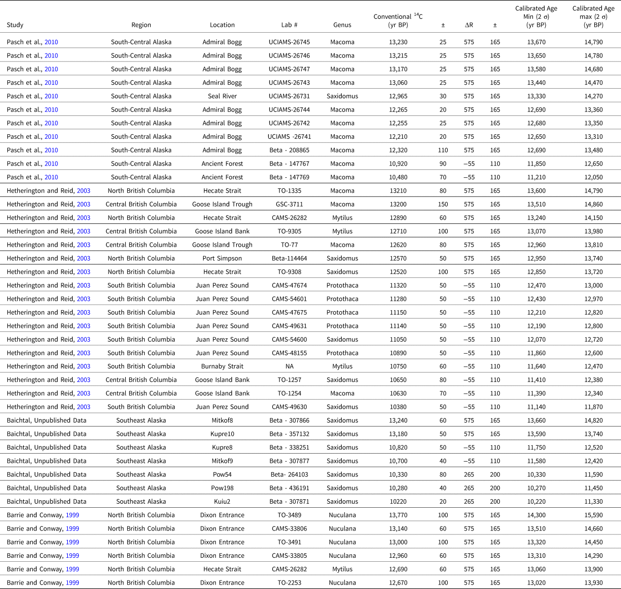
Recalibrating shellfish ages often has a direct impact on paleoclimate reconstructions. For example, the deglaciation of the Dixon Entrance separating Prince of Wales Island and Haida Gwaii is constrained using uncalibrated dates on marine fossils collected by Barrie and Conway (Reference Barrie and Conway1999). Cold-water foraminifera (Cassidulina reniforme) in ice-proximal sediments are dated at 14,380 ± 110 14C yr BP / 15,260–16, 370 cal yr BP, while the earliest clam (Nuculana fossa) marks the return to open water by 13,770 ± 100 14C yr BP / 14,320–15,580 cal yr BP.
The postglacial recolonization of the Northwest Coast by shellfish is also an important factor for the viability of the region for human settlement (Dyke et al., Reference Dyke, Dale and McNeely1996; Hetherington et al., Reference Hetherington, Barrie, Reid, MacLeod, Smith, James and Kung2003; Potter et al., Reference Potter, Reuther, Holliday, Holmes, Miller and Schmuck2017). Species traditionally consumed by Northwest Coast groups (e.g., Macoma nasuta, Saxidomus gigantea) appear to have recolonized rapidly across the entire Northwest Coast (Table 3). In South-Central Alaska, the oldest dated specimens are at 13,230 ± 25 14C yr BP / 13,670–14,790 cal yr BP (Pasch et al., Reference Pasch, Foster and Irvine2010), in Southeast Alaska at 13,240 ± 60 14C yr BP / 13,660–14,820 cal yr BP (J.F. Baichtal, unpublished data), and in British Columbia at 13,210 ± 80 14C yr BP/ 13,600–14,790 cal yr BP (Hetherington and Reid, Reference Hetherington and Reid2003). While we lack terrestrial samples from these slightly older contexts to produce paired-sample reservoir corrections, we note the overlap between the earliest food clams in Southeast Alaska (13,660–14,280 cal yr BP) and the last pagophilic Ring Seal remains from Shuká-Kaa Cave (13,970–15,700 cal yr BP, calibrated in Supplemental Table S8) as proxies for the elimination of substantial sea-ice in the region.
Table 3. Post-glacial recolonization of Northwest Coast waters by “food clams.”
In practice, choice of which ΔR value to use to calibrate unpaired shells requires careful consideration. For example, for samples with conventional radiocarbon dates near the BA-YD transition, a YD sample correction is implied: if the sample were from the BA, it would have been strongly affected by the MRE and would thus not report a conventional radiocarbon date close to the YD. In contrast, the transition between the YD and the EH has a high potential for overlapping radiocarbon dates. A sample of Early Holocene age is likely to have a high reservoir effect, resulting in a conventional radiocarbon date that appears to be within the YD. A sample of YD age, with a much lower MRE, could report a similar conventional radiocarbon age. Because ΔR values were at their lowest at the onset of the EH, YD calibrations should be appropriate for those samples reporting YD radiocarbon ages. As an exercise, we calibrated shells from this overlap zone with both corrections, and results were statistically the same at a 95% confidence interval (due to high overlapping uncertainties).
MRE corrections for mixed-diets in humans and bears on the Northwest Coast
Shuká-Kaa
MRE corrections are commonly used to calibrate radiocarbon ages on paleontological and archaeological mixed feeders: specimens that consumed marine species as a significant part of their diet (Dixon et al., Reference Dixon, Heaton, Lee, Fifield, Coltrain, Kemp, Owsley, Parrish, Turner, Edgar, Owsley and Jantz2014). This is of critical importance to Early Holocene archaeology on the Northwest Coast given the importance of cave sites (El Capitan Cave, K1 Cave, Gaadu Din 2, etc.) with paleontological and archaeological bear bone (Heaton and Grady, Reference Heaton, Grady, Schubert, Mead and Graham2003; Fedje et al., Reference Fedje, Mackie, Lacourse and McLaren2011). Few human remains from Southeast Alaska have been radiocarbon dated, with the notable exception of the Early Holocene Shuká-Kaa individual found on Prince of Wales Island. This individual's isotope values are typically interpreted as evidence of a ‘marine diet’ (Dixon et al., Reference Dixon, Heaton, Lee, Fifield, Coltrain, Kemp, Owsley, Parrish, Turner, Edgar, Owsley and Jantz2014; Potter et al., Reference Potter, Reuther, Holliday, Holmes, Miller and Schmuck2017). Given the difference between the Southeast Alaska Early Holocene ΔR average (265 ± 200) and McNeely et al.'s (2006) Southeast Alaska historic average (ΔR 360 ± 80, t (31) = 2.044, p = .049) used in the most recent calibration of the individual's age (Dixon et al., Reference Dixon, Heaton, Lee, Fifield, Coltrain, Kemp, Owsley, Parrish, Turner, Edgar, Owsley and Jantz2014), we provide an updated calibration using our new Early Holocene data. The pooled mean of the two radiocarbon dates reported for the skeleton (9820 ± 40 14C yr BP) was calibrated using our Early Holocene Southeast Alaska ΔR (265 ± 200) with the Mixed-Marine Northern Hemisphere Calibration Curve (Reimer et al., Reference Reimer, Austin, Bard, Bayliss, Blackwell, Bronk Ramsey, Butzin, Cheng, Edwards, Friedrich, Grootes, Guilderson, Hajdas, Heaton, Hogg, Hughen, Kromer, Manning, Muscheler, Palmer, Pearson, van der Plicht, Reimer, Richards, Scott, Southon, Turney, Wacker, Adolphi, Büntgen, Capano, Fahrni, Fogtmann-Schulz, Friedrich, Köhler, Kudsk, Miyake, Olsen, Reinig, Sakamoto, Sookdeo and Talamo2020), in light of the individual's marine diet (see below discussion).
We use our full Early Holocene Southeast Alaska calibration because we cannot rule out that the individual's diet did not include karst-influenced marine foods, particularly given their final resting place on karst-rich Prince of Wales Island. Our reevaluation of the individual's age is 9640–10,860 cal yr BP (two sigma). While the median age is comparable to that reported elsewhere (usually only discussed in relation to an average age of ca. 10,300 cal yr BP, most recently 10,230 ± 110 cal yr BP in Dixon et al., Reference Dixon, Heaton, Lee, Fifield, Coltrain, Kemp, Owsley, Parrish, Turner, Edgar, Owsley and Jantz2014), our estimate of the error more accurately reflects the considerable uncertainty produced by the diet-based calibration process (Russell et al., Reference Russell, Cook, Ascough, Scott and Dugmore2011).
Isotopic data from two dated elements of the Shuká-Kaa skeleton, dated to ca. 9800 14C yr BP, have long been used to support the marine diet of the Early Holocene human inhabitants of the region, based on carbon isotope values in Dixon et al.'s (Reference Dixon, Heaton, Fifield, Hamilton, Putnam and Frederick1997) report (δ13C = -12.5‰ for the mandible and -12.1‰ for the pelvis). New C- and N-isotope ratios have been published recently for the Shuká-Kaa individual (Dixon et al., Reference Dixon, Heaton, Lee, Fifield, Coltrain, Kemp, Owsley, Parrish, Turner, Edgar, Owsley and Jantz2014). Following the publication of these results, a robust sample of Mid- to Late Holocene individuals from coastal and interior British Columbia with a more nuanced model for diet determinations was also published—an ideal comparative sample (Schwarcz et al., Reference Schwarcz, Chisholm and Burchell2014a). The Shuká-Kaa individual's isotope data fit squarely among the salmonid-focused individuals of coastal British Columbia, rather than among those with a marine-mammal-heavy diet (Figure 8). These results are not unlike that of the Early Holocene Kennewick Man (Schwarcz et al., Reference Schwarcz, Stafford, Knuf, Chisholm, Longstaffe, Chatters, Owsley, Owsley and Jantz2014b), whose isotope ratios similarly were driven by anadromous fish, 500 km up the Columbia River. Particularly when human remains are the samples in question, it is important that measured radiocarbon ages are corrected appropriately, with adequate recognition of the potential influence of diet-driven reservoir effects.

Figure 8. (color online) Modified from Schwarcz et al., Reference Schwarcz, Chisholm and Burchell2014a. Isotopic analysis of prehistoric human skeletons compared to potential food sources along the Northwest Coast. Schwarcz et al. (Reference Schwarcz, Chisholm and Burchell2014a) argued that the influence of freshwater fish is driving the high 13C values of Kennewick Man. Isotope values of the Shuká-Kaa individual match individuals from prehistoric sites along coastal British Columbia, interpreted as having diets dominated by anadromous fish consumption.
Schwarcz et al. (Reference Schwarcz, Chisholm and Burchell2014a) note that nitrogen values in their samples suggest that mollusks never constituted more than 25% of the diet of their sampled coastal foragers (in favor of other marine food sources), yet the reservoir corrections applied to ancient human remains from the coast are inevitably derived from mollusks. Recognition that reservoir effects across fish and marine mammal species are also significantly different from shellfish (and one another) demands more diet-appropriate reservoir corrections for ancient human remains (Dumond and Griffin, Reference Dumond and Griffin2002; Clark et al., Reference Clark, Horstmann and Misarti2019; Dyke et al., Reference Dyke, Savelle, Szpak, Southon, Howse, Desrosiers and Kotar2019; Reuther et al., Reference Reuther, Shirar, Mason, Anderson, Coltrain, Freeburg, Bowers, Alix, Darwent and Norman2020). Because marine (likely anadromous) fish appear to be central to the diet of Shuká-Kaa and Kennewick Man (and not marine mammals, terrestrial mammals, freshwater fish, or mollusks), a marine reservoir correction based on anadromous fish is necessary (Figure 8).
A salmon-derived reservoir effect has yet to be quantified in detail. Southon and Fedje (Reference Southon and Fedje2003) included two historic salmon dates in their dataset (which we excluded from our mollusk synthesis). One pair has an R(t) of 870 ± 90, the other 1050 ± 85, for a weighted average R(t) of 970 ± 60. de Flamingh et al. (Reference de Flamingh, Mallott, Roca, Boraas and Malhi2018) recently dated a set of Late Holocene salmon bones from a house storage pit on the Kenai Peninsula, Alaska, commenting that their age was offset from two radiocarbon dates on wood from the house structure. Assuming the younger of the two wood dates most accurately reflects the age of storage pit usage, their paired sample has an R(t) of 950 ± 45. These few pairs strongly suggest that our present mollusk-derived MRE correction is insufficient for diet-based calibrations. Future production of a reservoir correction for salmon would provide more appropriate corrective values for mixed-feeders on the Northwest Coast. Anadromous fish spend part of their life cycle in freshwater streams and lakes, and the remainder in the North Pacific; such a project should include modern samples from karst and non-karst drainages alongside ancient samples, which could be assembled from well-dated archaeological contexts.
Post-glacial bear recolonization
In addition to humans, bears represent mixed-feeder species of great interest to the post-glacial history of the Northwest Coast. Radiocarbon dating of the earliest paleontological remains of black and brown bears found in caves in Southeast Alaska and British Columbia has the potential to track the recolonization of the region by these species, which is critical given recent evidence that pre-glacial lineages did not survive glaciation in refugia (Lindqvist, Reference Lindqvist2019). These omnivores serve as proxy indicators of a post-glacial environment that could have supported humans, making their presence of interest to archaeologists as well (Fedje et al., Reference Fedje, Mackie, Lacourse and McLaren2011). Unfortunately, published data on stratigraphic relationships are insufficient to link dated salmon and bear remains with charcoal, which could have produced sample-pairs for MRE calculation. As with humans, it remains unclear whether a mollusk-derived MRE correction is sufficient for calibration of radiocarbon dates on specimens with marine diets.
If calibrations accounting for a 50% mixed-feeder diet are applied to brown bears (following Heaton and Grady, Reference Heaton, Grady, Schubert, Mead and Graham2003), brown bears can be recalibrated using our values for comparison against the terrestrial diets of black bears (Table 4). In Southeast Alaska, the earliest brown and black bear dates overlap at two sigma (brown bear 13,310–14,000 cal yr BP; black bear 13,220–13,530 cal yr BP). A similar pattern is repeated on Haida Gwaii, overlapping these dates at two sigma, although Fedje et al. (Reference Fedje, Mackie, Lacourse and McLaren2011) reported stratigraphically older, abundant but undated brown bear remains in the Gaadu Din caves. A significantly older bear in the K1 Cave is dated to 16,500–17,200 cal yr BP (calibrated using BA ΔR 575 ± 165, assuming mixed diet, as indicated in Ramsey et al., Reference Ramsey, Griffiths, Fedje, Wigen and Mackie2004), likely the same individual reported by Wigen (Reference Wigen, Fedje and Mathewes2005) given the statistically identical age. At this time, while Haida Gwaii was deglaciated, ice was just receding from the outer coast of Southeast Alaska (Lesnek et al., Reference Lesnek, Briner, Lindqvist, Baichtal and Heaton2018). Given recent genetic evidence of late glacial interbreeding between the brown bears of Southeast Alaska and polar bears (Cahill et al., Reference Cahill, Stirling, Kistler, Salamzade, Ersmark, Fulton, Stiller, Green and Shapiro2015, Reference Cahill, Heintzman, Harris, Teasdale, Kapp, Soares and Stirling2018), this may represent a polar/brown bear hybrid.
Table 4. Post-glacial recolonization of the Northwest Coast by brown bears (mixed marine diet) and black bears (terrestrial diet).

CONCLUSION
Approaches to MRE models range from a broad global level (Butzin et al., Reference Butzin, Prange and Lohmann2005; Alves et al., Reference Alves, Macario, Urrutia and Cardoso2019; Reimer et al., Reference Reimer, Austin, Bard, Bayliss, Blackwell, Bronk Ramsey, Butzin, Cheng, Edwards, Friedrich, Grootes, Guilderson, Hajdas, Heaton, Hogg, Hughen, Kromer, Manning, Muscheler, Palmer, Pearson, van der Plicht, Reimer, Richards, Scott, Southon, Turney, Wacker, Adolphi, Büntgen, Capano, Fahrni, Fogtmann-Schulz, Friedrich, Köhler, Kudsk, Miyake, Olsen, Reinig, Sakamoto, Sookdeo and Talamo2020) to the very local (e.g., Edinborough et al., Reference Edinborough, Martindale, Cook, Supernant and Ames2016). Here we considered surface ocean reservoir effect data at a broad regional level by combining datasets that are expected to have been affected by comparable oceanic and glacial effects along the length of the Northwest Coast of North America, from the Southeast Alaska panhandle to Vancouver Island, British Columbia. R(t) and ΔR values for the Mid- and Early Holocene in southern Southeast Alaska are in close agreement with those from adjacent Haida Gwaii and Prince Rupert Harbor sampling localities in British Columbia. The aggregated data for the Northwest Coast on the whole present clear temporal trends, possibly driven by coastal upwelling.
The reservoir effect is strongest during the initial period of high productivity in the Bølling-Allerød, coinciding with Meltwater Pulse 1A (Barron et al., Reference Barron, Bukry, Dean, Addison and Finney2009; Davies et al., Reference Davies, Mix, Stoner, Addison, Jaeger, Finney and Wiest2011; Stanford et al., Reference Stanford, Hemingway, Rohling, Challenor, Medina-Elizalde and Lester2011; Addison et al., Reference Addison, Finney, Dean, Davies, Mix, Stoner and Jaeger2012; Walczak et al., Reference Walczak, Mix, Cowan, Fallon, Keith Fifield, Alder, Du, Haley, Hobern, Padman, Praetorius, Schmittner, Stoner and Zellers2020). The YD brought a decrease in productivity alongside cooled and freshened sea-surface waters, a signal of persistent local meltwater events (Praetorius et al., Reference Praetorius, Condron, Mix, Walczak, McKay and Du2020). The coinciding disruption to deep water ventilation appears to have lessened coastal upwelling significantly, resulting in lower levels of 14C-depleted DIC in coastal waters and allowing the MRE on the Northwest Coast to decrease to near ΔR 0, the global average. The end of the YD saw a return of coastal upwelling. Shellfish reservoir values steadily increased from the YD low, stabilizing by 8800 cal yr BP around a regional average that persisted through the Holocene. The updated reservoir effect estimates reported here will help refine regional chronologies of many types that are ultimately based on these common index fossils.
Supplementary material
To view supplementary material for this article, please visit https://doi.org/10.1017/qua.2020.131
Acknowledgments
The samples analyzed in this project were gathered across the Tongass National Forest by a range of researchers in collaboration with the U.S. Forest Service, including Risa J. Carlson and Jane Smith. Because a portion of the radiocarbon dates for this project were completed through collaboration with the Centre for Applied Isotope Studies at the University of Georgia, we would like to thank Alex Cherkinsky, Jeff Speakman, and the CAIS staff for their invaluable assistance. We also thank Maureen Walczak, Jeff Pigati, and our third anonymous reviewer for their time and constructive comments.
Financial Support
Funding was provided in part by a University of Alaska Museum of the North Geist Fund Grant, an Alaska Quaternary Center Travel Grant, and the Tongass National Forest Geology Program of the U.S. Forest Service.


