INTRODUCTION
The last glacial maximum (LGM), which occurred ca. 26.5–19 ka (Clark et al., Reference Clark, Dyke, Shakun, Carlson, Clark, Wohlfarth, Mitrovica, Hostetler and McCabe2009), remains somewhat poorly understood in Australian late Quaternary paleoenvironmental records (Reeves et al., Reference Reeves, Barrows, Cohen, Kiem, Bostock, Fitzsimmons, Jansen, Kemp, Krause and Petherick2013), despite being an example of a prominent, extreme climate event (Barrows and Juggins, Reference Barrows and Juggins2005). In the context of the Southern Hemisphere, it has been suggested that the onset of cold and dry climates was earlier (ca. 35–30 ka; Petherick et al., Reference Petherick, Moss and McGowan2011) than the equivalent Northern Hemisphere conditions. The timing of the climatic shift in the Southern Hemisphere is based on proxy records indicating increased aridity along the eastern margin of Australia (e.g., Colhoun et al., Reference Colhoun, Pola, Barton and Heijnis1999; Kershaw et al., Reference Kershaw, McKenzie, Porch, Roberts, Brown, Heijnis, Orr, Jacobsen and Newall2007b; Petherick et al., Reference Petherick, McGowan and Moss2008) and internationally (e.g., Denton et al., Reference Denton, Heusser, Lowel, Moreno, Andersen, Heusser, Schlühter and Marchant1999; Vandergoes et al., Reference Vandergoes, Newnham, Preusser, Hendy, Lowell, Fitzsimons, Hogg, Kasper and Schlüchter2005). The ensuing LGM was characterized by lowering of sea-level (Grant et al., Reference Grant, Rohling, Ramsey, Cheng, Edwards, Florindo, Heslop, Marra, Roberts and Tamisiea2014; Lambeck et al., Reference Lambeck, Rouby, Purcell, Sun and Sambridge2014), reduced precipitation (Hesse et al., Reference Hesse, Magee and Van Der Kaars2004), expansion of the continental landmass, and cooler climates across much of the Australian continent (Galloway, Reference Galloway1965; Bowler, Reference Bowler1976; Kemp and Spooner, Reference Kemp and Spooner2007). However, recent comparative studies of paleoenvironmental records have highlighted the need for robust chronological frameworks because site-specific proxy responses can be complex and hinder deeper understanding of how the LGM influenced the magnitude of environmental change in different regions (Harrison, Reference Harrison1993; Turney et al., Reference Turney, Haberle, Fink, Kershaw, Barbetti, Barrows, Black, Cohen, Correge and Hesse2006a; Williams et al., Reference Williams, Cook, van der Kaars, Barrows, Shulmeister and Kershaw2009; Reeves et al., Reference Reeves, Barrows, Cohen, Kiem, Bostock, Fitzsimmons, Jansen, Kemp, Krause and Petherick2013).
In order to unravel the complex history of Australian environmental change, it is essential to distinguish between locally driven proxy responses (e.g., change in vegetation cover, fire regimes, topographical influences) and those induced by large-scale shifts in the climate system (Svitok et al., Reference Svitok, Hrivnák, Oťaheľová, Dúbravková, Paľove-Balang and Slobodník2011). The challenge is that environmental change may be explained by both local and regional forces; for example, vegetation change may result from local fire regime changes or moisture balance shifts forced by regional climate. Deconvolution between local and regional drivers is important when investigating dust flux as the net mobilization of lithogenic material can be a result of processes at the source (e.g., Washington et al., Reference Washington, Todd, Lizcano, Tegen, Flamant, Koren and Ginoux2006) and depositional locus (Farebrother et al., Reference Farebrother, Hesse, Chang and Jones2017). Two ways to separate local and regional signals are to: (1) increase the current multi-proxy paleoenvironmental dataset for the LGM in Australia (Turney et al., Reference Turney, Haberle, Fink, Kershaw, Barbetti, Barrows, Black, Cohen, Correge and Hesse2006a), with particular emphasis on capturing records of sufficient antiquity in underrepresented and climatically sensitive locations; and (2) establish robust chronologies, in combination with multi-proxy datasets, which can be used to infer changes in local variables (e.g., effective precipitation, temperature, catchment conditions, and available moisture) and how they have influenced the paleoenvironmental record.
Lake sediments are important archives of paleoenvironmental information, capable of preserving a multitude of proxies from which, regional, local, and global climate dynamics can be inferred (Reeves et al., Reference Reeves, Barrows, Cohen, Kiem, Bostock, Fitzsimmons, Jansen, Kemp, Krause and Petherick2013). The benefit of lake archives is that they have the capacity to accumulate temporally high-resolution changes through time (Schnurrenberger et al., Reference Schnurrenberger, Russell and Kelts2003). However, it is not uncommon for lake sediment records to preserve unconformities due to depositional hiatuses, erosional episodes, or both (Kershaw et al., Reference Kershaw, van der Kaars, Moss, Opdyke, Guichard, Rule and Turney2006; Moss and Kershaw, Reference Moss and Kershaw2007; Mandl et al., Reference Mandl, Shuman, Marsicek and Grigg2016). To effectively interrogate paleoenvironmental records from lakes, it is critical to establish an understanding of how lake catchments evolve and how these changes may influence deposition through time (Birks and Birks, Reference Birks and Birks2006). In instances where there is a hiatus in the lake sediment record, the missing information can sometimes be inferred from other associated deposits (e.g., marginal dunes; Fitzsimmons et al., Reference Fitzsimmons, Bowler, Rhodes and Magee2007). However, for this approach to be effective, robust age controls are needed for the complementary sedimentary archives (Hesse, Reference Hesse2016).
Many unique biological and geochemical proxies are available within lacustrine sediments, from which physical and chemical analyses can provide insights into environmental change through time. Specific examples of biological proxies often investigated include pollen and charcoal (Kershaw et al., Reference Kershaw, McKenzie, Brown, Roberts and van der Kaars2010; Ellerton et al., Reference Ellerton, Shulmeister, Woodward and Moss2017; Lisé-Pronovost et al., Reference Lisé-Pronovost, Fletcher, Mallett, Mariani, Lewis, Gadd, Herries, Blaauw, Heijnis and Hodgson2019; Xiao et al., Reference Xiao, Yao, Hillman, Shen and Haberle2020), diatoms (Gasse and Van Campo, Reference Gasse and Van Campo2001; Song et al., Reference Song, Kong, Hu, Wang and Yang2020), and stable isotopes of sediments and preserved organisms (Zhang et al., Reference Zhang, Chen, Holmes, Li, Guo, Wang, Li, Lü, Zhao and Qiang2011; Long et al., Reference Long, Wood, Williams, Kalish, Shawcross, Stern and Grün2018). Analysis of terrigenous particles (e.g., dust) and sedimentary depositional features can be used to evaluate exogenous and in-lake condition changes. Advances in analytical techniques now allow the identification of complex, fine-scale change in sedimentary sequences, including features associated with dust deposition. Moreover, dust characterization from lake records provides a means to trace source locations, thereby providing an important understanding of wind regimes and environmental change in at the source location through time (e.g., McGowan et al., Reference McGowan, Petherick and Kamber2008; Petherick et al., Reference Petherick, Moss and McGowan2011).
Identifying changes in lake sediments, particularly those predominantly composed of organic matter, can be challenging because changes in sedimentology may be inconspicuous. In instances when sedimentology is unclear or complex, the application of micro-XRF core scanning (μXRF) can provide high-resolution (sub-millimeter) sediment geochemistry without the need for destructive sampling (Croudance and Rothwell, Reference Croudance and Rothwell2015). The success of applying μXRF to analyze finely laminated sediment archives has been demonstrated in a range of key paleoenvironmental studies, including climate change (e.g., Kylander et al., Reference Kylander, Ampel, Wohlfarth and Veres2011; Lauterbach et al., Reference Lauterbach, Brauer, Andersen, Danielopol, Dulski, Hüls, Milecka, Namiotko, Obremska and Von Grafenstein2011), anthropogenic disturbance (e.g., Guyard et al., Reference Guyard, Chapron, St-Onge, Anselmetti, Arnaud, Magand, Francus and Mélières2007; Niemann et al., Reference Niemann, Matthias, Michalzik and Behling2013), identification of pyroclastic material (e.g., Vogel et al., Reference Vogel, Zanchetta, Sulpizio, Wagner and Nowaczyk2010; McCanta et al., Reference McCanta, Hatfield, Thomson, Hook and Fisher2015), and changes in lake oxygenation conditions (e.g., Davies et al., Reference Davies, Lamb, Roberts, Croudace and Rothwell2015).
Interpretation of geochemical data obtained using μXRF requires careful consideration, particularly in sediments where composition is highly variable (Boyle, Reference Boyle, Last and Smol2002). Lighter elements in particular can be influenced by changes in water and organic content (Tjallingii et al., Reference Tjallingii, Röhl, Kölling and Bickert2007; Weltje and Tjallingii, Reference Weltje and Tjallingii2008), the effects of which can be minimized by normalizing to the total sum of Compton and Rayleigh scatter (incoherent and coherent scatter: inc/coh) (e.g., Kylander et al., Reference Kylander, Lind, Wastegård and Löwemark2012; Jouve et al., Reference Jouve, Francus, Lamoureux, Provencher-Nolet, Hahn, Haberzettl, Fortin, Nuttin and Team2013). Moreover, the setting of the catchment (e.g., local geology and lake-water properties) must be considered when inferring changes in any element quantified using μXRF, particularly because post-depositional changes in lake and catchment conditions can influence geochemistry (Kylander et al., Reference Kylander, Ampel, Wohlfarth and Veres2011).
Geochemical studies from wetlands on North Stradbroke Island show that variations in sediment chemistry are strongly influenced by aeolian influx (e.g., McGowan et al., Reference McGowan, Petherick and Kamber2008; Petherick et al., Reference Petherick, McGowan and Kamber2009; Kemp et al., Reference Kemp, Tibby, Arnold, Barr, Gadd, Marshall, McGregor and Jacobsen2020; Lewis et al., Reference Lewis, Tibby, Arnold, Barr, Marshall, McGregor, Gadd and Yokoyama2020). Trace element geochemistry of the inorganic sediment fraction from Native Companion Lagoon found the origin of the material was both from the Australian continent, important for providing context during the LGM, and local dunes (McGowan et al., Reference McGowan, Petherick and Kamber2008). Subsequent models of aeolian transportation pathways to North Stradbroke Island (Petherick et al., Reference Petherick, McGowan and Kamber2009) support this finding, with dust records now improving the understanding of regional climate during the LGM in coastal subtropical Australia (McGowan et al., Reference McGowan, Petherick and Kamber2008; Petherick et al., Reference Petherick, Moss and McGowan2011, Reference Petherick, Moss and McGowan2017; Kemp et al., Reference Kemp, Tibby, Arnold, Barr, Gadd, Marshall, McGregor and Jacobsen2020; Lewis et al., Reference Lewis, Tibby, Arnold, Barr, Marshall, McGregor, Gadd and Yokoyama2020).
This study examines environmental changes associated with climate variability since MIS 5 from Brown Lake, North Stradbroke Island, using a combination of geochemistry (μXRF core scanning) and geochronology (optically stimulated luminescence [OSL] and radiocarbon [14C] dating). The potential of Brown Lake for improved regional reconstructions of LGM conditions was highlighted by an initial OSL age of 47 ka for the base of the sediment sequence (Tibby et al., Reference Tibby, Barr, Marshall, McGregor, Moss, Arnold and Page2017). Moreover, there is limited information regarding the timing of dune emplacement proximal to Brown Lake and other wetlands on North Stradbroke Island. The aims of this study are three-fold: (1) to develop the first Bayesian age-depth model for the Brown Lake sediment; (2) to compare dust deposition in Brown Lake with nearby wetlands, to infer the history of late Pleistocene local dust deposition on North Stradbroke Island; and (3) to undertake direct OSL dating of dune fields, which host wetland sediment archives, in order to improve the spatial and temporal coverage of existing paleoenvironmental records for North Stradbroke Island. This will be achieved by examining high-resolution geochemical measurements from cores extracted at two different locations along the longitudinal axis of the water body. The separation between the cores will enable spatial changes attributed to basin evolution to be considered when investigating changes in moisture balance at both local and regional scales.
Study Sites
North Stradbroke Island is situated ~30 km east of the city of Brisbane, Queensland and is the second largest sand island in the world (Fig. 1a). North Stradbroke Island is positioned in the subtropics with mean annual summer and winter temperatures between 22–30°C and 12–20°C, respectively (BOM, 2019). The dominant wind direction is the south-east, driven by onshore trade winds (Colls and Whitaker, Reference Colls and Whitaker1990). Winter months on North Stradbroke Island are mild and dry with a large proportion of annual precipitation (1545 mm; BOM, 2019) occurring during the warm, humid summer and autumn seasons.
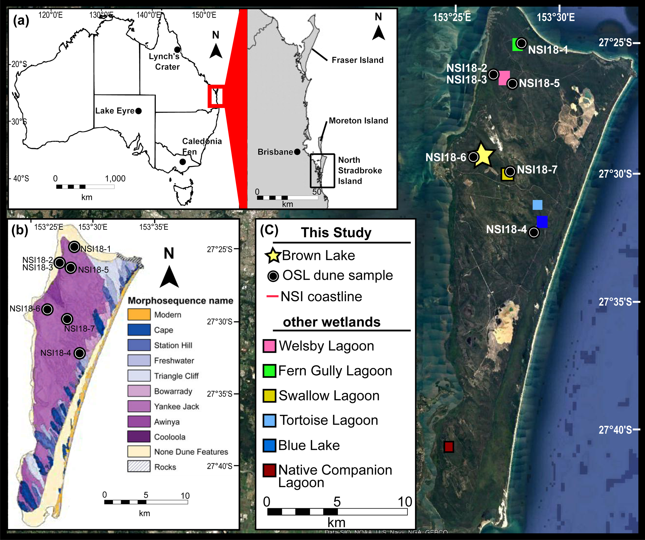
Figure 1. Location of North Stradbroke Island, dune sample sites, and locations referenced in text. (a) Position of the island in relation to Australia, outlined by a red square. (b) Dune field map adapted from Patton et al. (Reference Patton, Ellerton and Shulmeister2019), overlain by the OSL sample sites in this study. (c) Satellite image of North Stradbroke Island (source: Google Earth) and the position of wetlands referenced in text. (For interpretation of the references to color in this figure legend, the reader is referred to the web version of this article.)
North Stradbroke Island is part of the extensive south-east Queensland dune system that includes Fraser Island, Moreton Island (Figure 1a), and the Cooloola Sand Mass (Ward, Reference Ward2006; Patton et al., Reference Patton, Ellerton and Shulmeister2019). The topography of North Stradbroke Island is, in part, determined by the overprinting of older dunes by more recent dune units, becoming younger towards the east coast; as inferred from morphological analysis (Ward, Reference Ward2006) and remote sensing (Patton et al., Reference Patton, Ellerton and Shulmeister2019) data (Fig. 1b). What remains less clear, however, is what mechanisms are responsible for dune development on North Stradbroke Island, within which numerous wetlands lie (Fig. 1c). This study presents ages for dunes adjacent to prominent wetlands and evaluates the timing of advancement in the context of key climate events, including climate and sea-level change (Grant et al., Reference Grant, Rohling, Ramsey, Cheng, Edwards, Florindo, Heslop, Marra, Roberts and Tamisiea2014).
Brown Lake (27°29′10″S, 153°26′01″E; 56 m a.s.l.) is a naturally acidic (pH = 4.85 ± 0.02; Mosisch and Arthington, Reference Mosisch and Arthington2001) perched, endorheic lake that lies within the Yankee Jack dune formation (Ward, Reference Ward2006; Patton et al., Reference Patton, Ellerton and Shulmeister2019). It is the largest lake on North Stradbroke Island and has a 1743 ha drainage basin (Leach, Reference Leach2011). Brown Lake has a maximum water depth of 8.3 m, which varies in concert with effective precipitation (Fig.2). The present-day vegetation consists of open sclerophyll woodland, with a canopy dominated by Eucalyptus and Allocasuarina (Clifford and Specht, Reference Clifford and Specht1979).
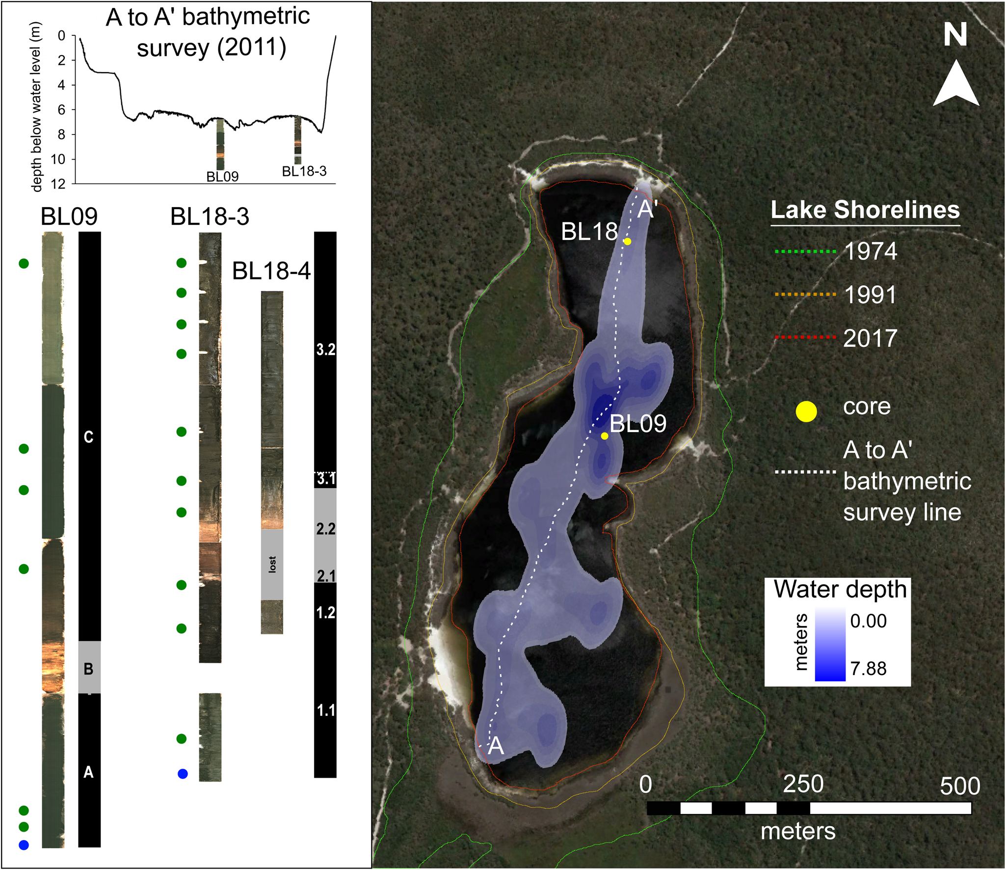
Figure 2. Position of sediment cores BL18 and BL09 recovered from Brown Lake. BL18 and BL09 cores placed on a 2011 bathymetric transect of Brown Lake. Optical images of BL18 and BL09 are shown next to position of radiocarbon samples (green circles), OSL samples (blue circles), and stratigraphic units (black and grey rectangles). Lake shorelines shown on the Google Earth satellite image were identified using historic aerial photos presented in Supplementary Figure S9. (For interpretation of the references to color in this figure legend, the reader is referred to the web version of this article.)
METHODS
Coring and Bathymetry
Lake sediment cores were extracted from Brown Lake in two expeditions taking place in 2009 and 2018 (Fig. 2). A single, 3.95 m core was extracted from the central point of the lake in 2009 (BL09) using a Livingstone Corer, capturing 1.0 m of sediment with each successive drive. Sediment from BL09 was extruded into PVC trays, wrapped in cling film, and transported to the University of Adelaide. In 2011, a bathymetric survey was undertaken using a boat-mounted sonar system (Altimeter: Tritech Int Ltd, Model PA500/6-S) attached to a data recorder (Rugged Brookhouse NMEA 0813) and a GPS (Garmin GPSMAP 60Cx), allowing bottom lake topography to be linked with the core locations. A follow-up coring expedition occurred in 2018, with the aim of acquiring sediment from the northern end of the basin along the 2011 bathymetric transect line (Fig. 2). The two cores were then used to generate a sedimentological profile of Brown Lake and evaluate subsurface heterogeneity. In order to increase the reliability of interpretations from the sediment collected in 2018, two parallel and vertically offset sediment cores (BL18-3 and BL18-4) were collected 2 m apart using a modified Bolivia piston corer aboard a Kawhaw floating platform. The sediment was extracted in one meter drives, with BL18-3 and BL18-4 reaching depths of 3.57 m and 2.73 m, respectively. To minimize sediment compaction and exposure to light, each drive was sealed in the core tube rather than being extruded in the field. The cores were split along their longitudinal axis under subdued red LED lighting to prevent daylight contamination and preserve sample integrity for subsequent OSL dating. One half of each core remained under strict lighting conditions (sealed in opaque black plastic) to prevent bleaching of the luminescence signal, while the other was used to conduct further, non-light-sensitive sampling.
Laboratory techniques
Physical properties of the sediment
Sediment descriptions were defined using standardized sedimentological terminology and characteristics based on analyzing the sediment both in the core and as a smear, where possible. Sediment properties (i.e., water content, bulk density, and the organic:inorganic ratio) were measured using loss on ignition (LOI) and evaluated at centimeter scale down the length of BL18-3 (n = 347). BL09 LOI samples were taken every two centimeters (n = 217). Samples were extracted as 1 cm3 of bulk sediment and measured following Heiri et al. (Reference Heiri, Lotter and Lemcke2001). This included weighing sediment before and after oven drying at 100°C and ashing at 550°C.
μXRF core scanning
Geochemical analysis was undertaken using a μXRF core scanner, measuring at millimeter resolution, at the Australian Nuclear Science and Technology Organisation (ANSTO) facility (see Supplementary Information for details). Elements of interest for this study were selected using the following criteria: (1) element ratios and element count data from μXRF scanning that represented chemical variation resulting from biogenic productivity (Ca/Ti, Br, Ca, inc/coh, Si/Ti) and siliciclastic influx (Rb, Al, Si, K, Ze, Fe, Ti) from within the sediment matrix were targeted (Hendy et al., Reference Hendy, Napier and Schimmelmann2015); (2) elements with large systematic uncertainties (e.g., influenced by the air gap between the sensor and the sediment) were removed from the dataset; and (3) elements and elemental ratios were categorized as intrinsic organic production indicators and extrinsically aeolian-derived lithic indicators—given that Brown Lake is a perched lake with no inflowing streams, sediment accumulation is a function of both. A principal component analysis (PCA) was undertaken on the selected suite of elements, which identified the inorganic component, represented by Axis 1 (PC1), as the major factor of sediment chemical composition (Supplementary Fig. S1). The statistical link between siliciclastic accumulations and element variation enabled direct comparisons with the nearby Fern Gully Lagoon and Welsby Lagoon (Fig.1c) sediment records where aeolian-derived material is a primary influence on sediment chemistry (Kemp et al., Reference Kemp, Tibby, Arnold, Barr, Gadd, Marshall, McGregor and Jacobsen2020; Lewis et al., Reference Lewis, Tibby, Arnold, Barr, Marshall, McGregor, Gadd and Yokoyama2020).
Core correlation
To overcome artificial breaks resulting from the coring process itself, the parallel and vertically offset cores BL18-3 and BL18-4 were combined using sequence slotting, hereafter denoted BL18. Sequence slotting was undertaken in CPLslot v2.4 (Hounslow and Clark, Reference Hounslow and Clark2016) using the μXRF values for Al, Si, Ca, and Br as input variables. These elements provided accurate estimates of detrital and biochemical input based on their positions and grouping on the PC1 axis for Brown Lake (Supplementary Fig. S1) and other sites on North Stradbroke Island (e.g., Kemp et al., Reference Kemp, Tibby, Arnold, Barr, Gadd, Marshall, McGregor and Jacobsen2020; Lewis et al., Reference Lewis, Tibby, Arnold, Barr, Marshall, McGregor, Gadd and Yokoyama2020). Element count data were normalized by inc/coh because this was found to correlate with measured LOI values (r2 = 0.90; p-value <0.05) (Supplementary Fig. S2), thus reducing the influence of water content and, or, organic matter on geochemistry.
The sequence slotting procedure included the following constraints: (1) the combined sequence started with the top of BL18-3; (2) the combined sequence ended with the bottom of BL18-3; and (3) BL18-4 was vertically offset from the surface by at least 0.5 m, and therefore did not overlap with BL18-3 above this depth. Additionally, a series of minor user choices were included in the sequence-slotting algorithm to accommodate the physical characteristics of the sediment in each core (i.e., sediment was lost between 2.02–2.50 m during retrieval of BL18-4 drive 2—likely a result of increased porosity at the base of the drive relative to BL18-3).
The BL09 and the BL18 cores were not correlated using sequence-slotting because of lithological differences in the sediment profiles (i.e., the presence of a large sand band in the BL18 cores, which was absent in BL09) and the distance between the two coring locations (Fig. 2). Therefore, comparisons between the BL18 and BL09 cores were based on stratigraphic similarities and were used primarily to interpret lake history and the extent of heterogeneous sedimentation along a basin transect.
Dating and age modeling
Radiocarbon dating was undertaken on the BL18-3 and BL09 profiles (Fig. 2) with measurements made on bulk sediment (2 cm3) due to a lack of macrofossils. Eleven bulk sediment samples from BL18-3 were analyzed at the ANSTO Accelerator Mass Spectrometry (AMS) facility, and six samples from BL09 were analyzed at Beta Analytic and the Waikato Radiocarbon Dating Laboratories. The samples were prepared using conventional approaches (see Supplementary Information for details), including standard ABA treatments (Brock et al., Reference Brock, Higham, Ditchfield and Ramsey2010). The 14C ages were calibrated to calendar years using OxCal v4.3.2 and the SHCal13 calibration curve (Bronk Ramsey, Reference Bronk Ramsey2009; Hogg et al., Reference Hogg, Hua, Blackwell, Niu, Buck, Guilderson, Heaton, Palmer, Reimer and Reimer2013).
Single-grain OSL dating was undertaken on quartz grains from a sample extracted from the base of BL18-3.3 and compared with the single-grain OSL age reported previously for BL09 (Tibby et al., Reference Tibby, Barr, Marshall, McGregor, Moss, Arnold and Page2017). An additional seven OSL samples were collected from the crest of dunes found adjacent to five prominent North Stradbroke Island wetlands (Fig. 1c). These dune samples were taken from areas with surface exposures classified as the Yankee Jack Formation (Ward, Reference Ward2006). Three OSL samples were collected from two different dune crests surrounding Welsby Lagoon in order to better constrain variability in dune emplacement and preservation dynamics.
The Brown Lake core sample was extracted under subdued red light conditions, with care taken to ensure contaminant grains from coring were not included in the final analysis, ~1 cm of sediment was removed from the exposed sediment core face, with sediment within 1 cm of the coring tube also excluded (this material was retained for dosimetric analysis). The dune samples were collected from freshly dug pits to enable three-dimensional assessments of stratigraphy and ensure that zones affected by extensive root systems and bioturbation were avoided. Dune crests were targeted to maximize the likelihood of sampling primary (non-reworked) aeolian deposits. Individual OSL samples were collected by hammering opaque PVC tubes into cleaned exposures of A2 and B Horizons at depths of 70–180 cm beneath the surface, taking care to avoid the modern root layer and active bioturbation zones (Supplementary Fig. S3). Approximately 500 g of additional bulk sediment was collected from the walls of each OSL sample hole (i.e., the surrounding ~2–3 cm of material in all directions) for evaluation of beta dose rate, secular equilibrium, and water content.
The environmental dose rates of the dune samples have been calculated using a combination of in situ field gamma-ray spectrometry and low-level beta counting. Gamma dose rates were determined from in situ measurements made using a Canberra NaI:Tl detector to account for any spatial heterogeneity in the surrounding (~30 cm diameter) gamma radiation field of each sample. The ‘energy windows’ approach described in Arnold et al. (Reference Arnold, Duval, Falguères, Bahain and Demuro2012) was used to derive individual estimates of U, Th, and K concentrations from the field gamma-ray spectra. External beta dose rates were determined from measurements made using a Risø GM-25-5 beta counter (Bøtter-Jensen and Mejdahl, Reference Bøtter-Jensen and Mejdahl1988) on dried and homogenized, bulk sediments collected directly from the OSL sampling positions. High-resolution gamma spectrometry was additionally performed on the dune samples to examine the state of secular equilibrium in the 238U and 232Th decay series.
Elemental concentrations and specific activities were converted to dose rates using accepted conversion factors (Guérin et al., Reference Guérin, Mercier and Adamiec2011). A small, assumed internal (alpha plus beta) dose rate component of 0.02 ± 0.01 Gy/ka has been included in the final dose rate calculation based on ICP-MS U and Th measurements made on etched quartz grains from nearby Welsby Lagoon (Lewis et al., Reference Lewis, Tibby, Arnold, Barr, Marshall, McGregor, Gadd and Yokoyama2020) and an alpha efficiency factor of 0.04 ± 0.01 (Rees-Jones, Reference Rees-Jones1995; Rees-Jones and Tite, Reference Rees-Jones and Tite1997). Cosmic-ray dose rates were calculated (Prescott and Hutton, Reference Prescott and Hutton1994), after taking into consideration lake water level, site altitude, geomagnetic latitude, and density and thickness of sediment overburden.
The final dose rates for the lake core and dune OSL samples have been corrected for beta-dose attenuation and long-term water content (Mejdahl, Reference Mejdahl1979; Aitken, Reference Aitken1998; Brennan, Reference Brennan2003). The long-term water content for the Brown Lake OSL sample was considered to be equivalent to the empirical values determined as part of the LOI procedures, with separate corrections applied to the beta, gamma, and cosmic dose rate terms (see Supplementary Table S1 for details). An assumed long-term water content of 7 ± 3% was applied to the NSI18 dune samples, following approaches used in comparable OSL dating studies of dune deposits from the region (e.g., Ellerton et al., Reference Ellerton, Rittenour, Shulmeister, Gontz, Welsh and Patton2020).
Purified quartz grains (Ø 180–212 μm or 212–250 μm) were prepared using procedures described in Lewis et al. (Reference Lewis, Tibby, Arnold, Barr, Marshall, McGregor, Gadd and Yokoyama2020), with single-grain equivalent dose (De) measurements undertaken using apparatus and conditions detailed in the Supplementary Information. Single-grain De values were determined using the single aliquot regenerative dose (SAR) procedure (Murray and Wintle, Reference Murray and Wintle2000), shown in Supplementary Table S2. Individual De values were only included in the final age calculation if they satisfied a series of widely accepted quality assurance criteria (Supplementary Table S3).
Bayesian age-depth models were produced for BL18 and BL09 cores in OxCal (Bronk Ramsey, Reference Bronk Ramsey2009; Bronk Ramsey and Lee, Reference Bronk Ramsey and Lee2013), following the procedures outlined in Lewis et al. (Reference Lewis, Tibby, Arnold, Barr, Marshall, McGregor, Gadd and Yokoyama2020) and discussed in the Supplementary Information. Separate depositional units have been included in the OxCal models for BL18 and BL09 on the basis of independent sedimentological and lithological interpretations (as detailed in the Results).
Brown Lake's sedimentological history, and the climate implications influencing deposition with respect to other North Stradbroke Island and Australian records, is discussed in relation to a subset of the eight phases identified through the OZ-INTIMATE climate synthesis (Reeves et al., Reference Reeves, Barrows, Cohen, Kiem, Bostock, Fitzsimmons, Jansen, Kemp, Krause and Petherick2013). We have combined the early and late deglacial phases and considered the Holocene as a whole (Reeves et al., Reference Reeves, Barrows, Cohen, Kiem, Bostock, Fitzsimmons, Jansen, Kemp, Krause and Petherick2013).
RESULTS
Lithology, physical and chemical properties
Sedimentology
The sediment units present in the BL18 (based on descriptions of BL18-3) and BL09 cores (Fig. 3) are broadly similar and are dominated by very dark-brown to black lake mud with fine- to coarse-grained sands incorporated within the sedimentary matrix. BL18 contains three distinct units, Unit 1 (3.57–2.29 m), Unit 2 (2.29–1.65 m), and Unit 3 (1.65–0 m), each of which contains two sub-units. BL09 also contains three units denoted Unit A (3.98–3.14 m), Unit B (3.14–2.67 m), and Unit C (2.67–0 m) (Moss, Reference Moss2013).

Figure 3. (color online) Optical images, sedimentary units, and properties of BL18 (black) and BL09 (grey) as measured using the loss on ignition approach. Graphs are aligned by depth and show sediment (a) moisture content, (b) bulk density, and (c) inorganic content.
The lowest units present in both cores (Unit 1 and Unit A; Fig. 3) are very dark-brown to black mud (10YR 2/2, 10YR 2/1) with a blocky texture. In the BL18 core, sub-unit 1.1 (3.57–2.69 m) gradually becomes increasingly pliable towards the top of the unit. Sub-unit 1.2 (2.69–2.29 m) is distinguished by a transition from clay to more silty texture and an increased abundance of fine-grained sand. Additionally, this unit also hosts a thin (4 mm wide) coarse-grained sand vein that is perpendicular to the bedding for ~20 cm from the top of the unit.
In the BL18 core, Unit 2 is distinguished from Unit 1 by an overall increase in the proportion of sand. The base of the unit is identified by the presence of a distinctive thin (6 cm), coarse-grained sand layer that contains intermixed angular black clasts (<1 mm) and light brown grains (Fig. 3) from 2.29 m. A distinctive contact with the underlying sub-unit 1.2 is identified by the juxtaposition of the grey-white sand (10YR 7/1) overlying very dark brown mud (7.5YR 2.5/2). This sand layer is designated sub-unit 2.1 (2.29–2.23 m) and is only present in the BL18 record. The shared sedimentology between BL18 and BL09 is re-established from sub-unit 2.2 (2.23–1.65 m) and Unit B (3.14–2.67 m) upwards (Fig. 3). The sedimentology of these units both increase in clay content up core with a decrease in the proportion of sand grains towards the surface more apparent in BL18. The sediment changes from the grey-white sand of sub-unit 2.1 into a dark brown (10YR 3/2) towards the middle, before grading into a black mud (10YR 2/1) towards the top. However, the color gradient is not as obvious in BL09, due to the as the absence of the underlying sandy layer.
The youngest, and thickest unit in the BL18 and BL09 cores is Unit 3 (1.65–0 m) and Unit C (2.67–0 m), respectively (Fig. 3). The base of this unit in BL18 is designated sub-unit 3.1 (1.65–1.55 m), which is characterized by the sediment having had transitioned from the mud of sub-unit 2.2 to a more organic-rich, silty clay-like texture. This subsequently transitions into the homogenous organic black (10YR 2/1) mud of sub-unit 3.2 (1.55–0 m). The change in texture between sub-unit 3.1 and 3.2 is concordant with the incorporation of very fine-grained sand material within the sediment matrix towards the top of Unit 3.
Moisture and organic content
The moisture and organic content of the BL18 and BL09 records reflect the sedimentary unit divisions (Fig. 3). The sediment from BL18 has a wider range of moisture content (15.5–90.6%wet), bulk density (0.5–2.8 g/cm3), and inorganic content (10.5–97.7%dry) than BL09 (41.1–87.2%wet; 1.1–2.4 g/cm3; 5.7–88.2%dry). Our analysis of these properties focusses on BL18 because this core sequence would have experienced less physical alteration during the core extraction in comparison to BL09, which was extruded in the field.
Unit 3 of BL18 has the highest moisture content of the three units of the same core, with a mean value of ~84% (Unit 2 and Unit 1 have mean values of 36% and 61%, respectively). Unit 2 has the highest inorganic content on average (91%dry), which is more than double that of Unit 3 (26%dry) and higher than Unit 1 (59%dry). The sandy Unit 2 has a mean bulk density of 1.8 g/cm3, which was considerably higher than that of Unit 3 and Unit 1 (both have an average of 1.4 g/cm3). This difference in bulk density likely reflects the influence of increased inorganic material having been deposited within the soil matrix of Unit 2.
μXRF elemental scanning and principal component analysis
The elemental counts from the μXRF core scanning of BL18 and BL09 exhibit amplitude changes that correspond with transitions between sedimentary units (Fig. 4, Supplementary Fig. S7). μXRF Rayleigh scattering (i.e., incoherent/coherent) had a strong correlation (r2 = 0.95, p-value <0.05; Supplementary Fig. S2) with organic matter content as determined by LOI. Elements of interest (see Methods) were subsequently incorporated into a PCA to evaluate their variability down core. Elements associated with clastic terrestrial origins had high loadings on PC1 (Supplementary Fig. S1). Additionally, the correlation between these elements (Supplementary Fig. S1) suggests that the sediment chemistry is strongly influenced by the influx of aeolian transported inorganic material, as observed in neighboring organic-rich wetland sediments (Kemp et al., Reference Kemp, Tibby, Arnold, Barr, Gadd, Marshall, McGregor and Jacobsen2020; Lewis et al., Reference Lewis, Tibby, Arnold, Barr, Marshall, McGregor, Gadd and Yokoyama2020). Geochemical variation driven by inorganic material deposition is further supported by the separate grouping of biogenic and lithogenic element proxies and ratios (Supplementary Fig. S1), particularly the low loading on PC1 for the organic indicator (i.e., inc/coh).

Figure 4. Scanning XRF elemental counts per second (CPS) of selected terrigenous elements (as identified using Principal Component Analysis). Aluminum elemental counts (grey line) overlain by a 10 point moving average (black line). Yellow and orange shading represent the sand (sub-unit 2.1) and transitional (sub-unit 2.2) layers observed in the BL18 sedimentary sequence, respectively. For biogenic element correlations the reader is directed to Supplementary Figure S8. (For interpretation of the references to color in this figure legend, the reader is referred to the web version of this article.)
Core correlation
Sequence-slotting successfully matched the element concentrations from BL18-4 to those in BL18-3, as shown in Supplementary Figure S10. The potential range of sequence-slotting configurations is demonstrated in the H-matrix (Supplementary Fig. S10) (Gordon, Reference Gordon1982) and represents all possible depths at which slotting could occur. For this study, the central correlative depth is taken from the H-matrix to represent the best fit of the two cores thus used to project the depths of BL18-4 onto those of BL18-3. The suitability of using this approach is also supported by the high delta value (0.828), indicating that the sequences were well matched.
Chronology
14C dating
The AMS 14C ages obtained for BL18 and BL09 are presented in Table 1. Overall, there is stratigraphic agreement between the 14C results from core BL18 and BL09. Moreover, the ages of replicate samples collected from the same depth in the BL18 core (OZX792/OZX793) overlap at 1σ. The 14C sample extracted from the bottom of the BL18 core (OZX794a) produced a 95.4% C.I. calibrated age range of 40,120–38,790 cal yr BP, which was confirmed with a replicate measurement (OZX794b = 40,400–39,070 cal yr BP). The 14C ages for this sample are systematically younger than the overlying replicate samples (OZX792, OZX793), which yielded replicate 95.4% C.I. calibrated age range of 48,790–45,620 cal yr BP and 49,830–46,710 cal yr BP, respectively. The cause of the inversion is currently uncertain and is possibly linked to sediment mixing from turbulence, humification, or both (Shore et al., Reference Shore, Bartley and Harkness1995).
Table 1. Radiocarbon (14C) ages for the samples extracted from BL18 and BL09 Brown Lake sediment cores, respectively. Ages have been calibrated against SHCal13 using the OxCal software (Bronk Ramsey, Reference Bronk Ramsey2009; Bronk Ramsey and Lee, Reference Bronk Ramsey and Lee2013; Hogg et al., Reference Hogg, Hua, Blackwell, Niu, Buck, Guilderson, Heaton, Palmer, Reimer and Reimer2013). All samples were treated using acid-base-acid (ABA) pre-treatments. The calibrated age range shown is the 95.4% probability range (combining two or more potential calibration ranges, where they exist).

a, bReplicate samples, which were combined in the Bayesian age-depth modelling using the OxCal ‘combine’ function.
cRounded to nearest ten years.
OSL dating
The results of the single-grain OSL De analysis and age determination are reported in Table 2 and Figure 5. The acceptance rate of grains for each OSL sample, following application of the SAR quality assurance criteria, ranged between 2–8% (Supplementary Table S3). Most samples (5 out of 8) exhibit relatively homogeneous single-grain De distributions with low overdispersion values of 18–20%. These overdispersion values are consistent with those typically reported for well-bleached and undisturbed single-grain De datasets at 2σ (e.g., the average overdispersion of 20 ± 1%; Olley et al., Reference Olley, Pietsch and Roberts2004; Arnold and Roberts, Reference Arnold and Roberts2009), as well as those reported for ‘ideal’ lacustrine samples from related North Stradbroke Island wetland localities (e.g., Kemp et al., Reference Kemp, Tibby, Arnold, Barr, Gadd, Marshall, McGregor and Jacobsen2020; Lewis et al., Reference Lewis, Tibby, Arnold, Barr, Marshall, McGregor, Gadd and Yokoyama2020). The final De values of these five samples (BL18-A, NSI18-1, NSI18-2, NSI18-3, and NSI18-6) have therefore been calculated using the central age model (CAM) (Galbraith et al., Reference Galbraith, Roberts, Laslett, Yoshida and Olley1999).
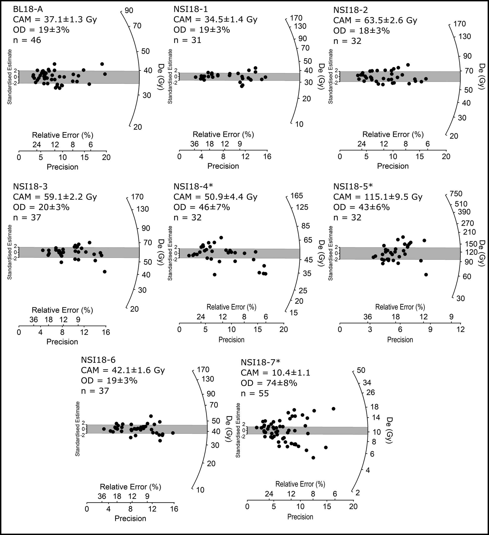
Figure 5. Radial plots showing the single-grain De distributions obtained for OSL samples from the BL18-3 core and NSI18 dunes. The grey shaded band on each plot is centered on the De value (in Gy) used for the final age calculation. For all samples, the De value has been calculated using the central age model (CAM) of Galbraith et al. (Reference Galbraith, Roberts, Laslett, Yoshida and Olley1999). For comparative purposes, the finite mixture model (FMM) dose components identified for samples marked with an asterisk (*) are shown in Supplementary Figure S5b.
Table 2. Dose rate data, equivalent doses (De), overdispersion values, and OSL ages for lacustrine samples from Brown Lake and dune samples from North Stradbroke Island. The final age for each sample is shown in bold, which has been derived using the age model considered to be most appropriate on statistical and interpretative grounds (see main text and Supplementary Tables S3–S6 for details).
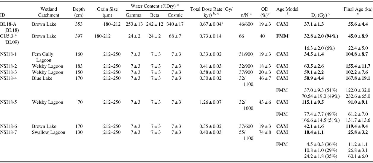
a Long-term water contents used for beta/gamma/cosmic-ray dose rate attenuation, respectively, expressed as% of dry mass of mineral fraction, with an assigned relative uncertainty of ± 5%. For sample BL18-A, the final beta dose rate has been adjusted for moisture attenuation using the measured water contents determined from the midpoint of the OSL sample depth. The final gamma dose rate has been adjusted using the average water content measured from the OSL sample midpoint, as well as from 1 cm3 bulk sediment samples collected for the overlying and underlying 10 cm depth. The final cosmic-ray dose rate has been adjusted using the average water content measured from 1 cm3 bulk sediment samples collected at 1 cm intervals throughout the overlying core sequence (refer to Fig. 3). For the NSI18 samples, beta, gamma, and cosmic dose rates have been corrected using a fixed long-term water content of 7 ± 3%, following approaches used in comparable OSL dating studies of dune deposits in the region (e.g., Ellerton et al., Reference Ellerton, Rittenour, Shulmeister, Gontz, Welsh and Patton2020).
b Individual dose rate components (i.e., gamma, beta, internal, and cosmic dose rate contributions) are outlined in Supplementary Table S1.
c Mean ± total uncertainty (68% confidence interval), calculated as the quadratic sum of the random and systematic uncertainties.
d Number of De measurements that passed the SAR quality assurance criteria and were used for De determination (n)/total number of grains analyzed (N).
e OD = overdispersion; the relative spread in the De dataset beyond that associated with the measurement uncertainties for individual De values.
f CAM = Central age model; FMM = Finite mixture model. See Supplementary Tables S4–S6 for details of the FMM fitting results. The FMM parameter values shown here were obtained from the optimum FMM fit (i.e., the fit with the lowest BIC score; Arnold and Roberts, Reference Arnold and Roberts2009). Percentage values shown in parentheses refer to the proportion of measured grains falling within each identified FMM dose component. The FMM dose component containing the highest proportion of accepted grains has been nominally selected for the final FMM De calculation; see main text for further discussions and sample-specific interpretations.
g Sample GU5.3 is taken from core BL09 and was originally presented in Tibby et al. (Reference Tibby, Barr, Marshall, McGregor, Moss, Arnold and Page2017). This sample is included for comparative purposes and is presented according to the information provided in the original publication.
Interestingly, the limited De scatter and low overdispersion obtained for Brown Lake sample BL18-A contrast with the De characteristics reported for sample GU5.3 from core BL09 (Tibby et al., Reference Tibby, Barr, Marshall, McGregor, Moss, Arnold and Page2017), despite being extracted from the same sediment body. Sample GU5.3 has an overdispersion of 40% (approximately twice that of BL18-A; 19 ± 3%), which was originally attributed to a combination of sediment disturbance (e.g., Arnold and Roberts, Reference Arnold and Roberts2011) and insufficient resetting of residual signals prior to burial (e.g., Arnold et al., Reference Arnold, Bailey and Tucker2007; Arnold and Roberts, Reference Arnold and Roberts2009). Given the homogenous De distribution we report for sample BL18-A, an alternative explanation for the GU5.3 De scatter might relate to the coring approach utilized (Tibby et al., Reference Tibby, Barr, Marshall, McGregor, Moss, Arnold and Page2017). Unlike the BL18 sediment, which was retained within the core tubes, the BL09 core was extruded in the field with limited protection from light exposure. Considering these contrasting sampling approaches, the BL09 sediment may have additionally experienced some vertical grain transfer or light contamination prior to OSL sampling, which could have given rise to a seemingly mixed or heterogeneously bleached De signature (incorporating both low and high De scatter). For the purpose of this study, we have included the originally published age for sample GU5.3 in our site assessment (45 ± 8.9 ka; Tibby et al., Reference Tibby, Barr, Marshall, McGregor, Moss, Arnold and Page2017) because it has been derived using a statistical age model designed to account for additional De scatter related to potential sampling contamination (finite mixture model; Galbraith and Green, Reference Galbraith and Green1990); although we note potential caveats regarding the original interpretation of this De dataset.
Three of the dune samples (NSI18-4, NSI18-5, NSI18-7) exhibit complex De distributions characterized by broad De scatter and high overdispersion values (43 ± 6% to 74 ± 8%) that do not overlap at 2σ with the site-specific ‘baseline’ estimates of underlying dose overdispersion determined from dune samples NSI18-1, NSI18-2, NSI18-3, and NSI18-6. Application of the FMM to these three De datasets also confirms the presence of multiple discrete dose components (Supplementary Tables S4–S6). Similar multimodal and scattered single-grain OSL De datasets have been reported elsewhere for the Cooloola Sand Mass (Walker et al., Reference Walker, Lees, Olley and Thompson2018), and have been interpreted as reflecting aeolian reactivation and localized reworking of original dune emplacements. This type of post-depositional mixing, whereby pre-existing aeolian deposits are incorporated into more recent dune building events, could be considered a possible explanation for some of the discrete dose components observed in samples NSI18-4, NSI18-5, and NSI18-7. However, given the low dose rates of these quartz-rich dune sands (Table 2), and the known presence of heavy minerals (zircons, monazites) and K-feldspar grains that could have acted as radioactivity hotspots in the Yankee Jack Formation (Thompson, Reference Thompson1981; Tejan-Kella et al., Reference Tejan-Kella, Chittleborough, Fitzpatrick, Thompson, Prescott and Hutton1990), it is feasible that this enhanced dose dispersion could have arisen from spatial variations in beta dose rates experienced by individual grains (e.g., Nathan et al., Reference Nathan, Thomas, Jain, Murray and Rhodes2003). Intrinsic sources of De scatter (e.g., Demuro et al., Reference Demuro, Arnold, Froese and Roberts2013) or bioturbation could have further contributed to the observed scatter in these three samples; though it is notable that such complications were not similarly observed in the other samples from these sites that displayed ideal De distributions (NSI18-1, NSI18-2, NSI18-3, and NSI18-6).
The difficulties of ascertaining the true underlying sources of De scatter for NSI18-4, NSI18-5, and NSI18-7, and the impracticalities of retrospectively calculating suitable dose rates for the identified multiple dose components, mean that use of the FMM for OSL age evaluation is not necessarily straightforward in this study. These interpretive complications are compounded by the fact that the identified components of each sample contain very similar proportions of grains (i.e., there are no clear dominant dose components). As a pragmatic solution, we have therefore used the CAM De and bulk (sample-averaged) dose rate to derive the final age estimates for NSI18-4, NSI18-5, and NSI18-7 (Table 2). For comparative purposes, Table 2 also shows the ages derived for these samples using the FMM components, assuming that the sample-averaged dose rates are broadly representative of those experienced by individual dose components during burial. This assumption may be reasonable given the shared local source of accumulated sediment in a given dune field, but further research would be required to demonstrate its suitability for the individual deposits under consideration here.
The CAM ages for samples NSI18-4 and NSI18-5 are broadly consistent (at 2σ) with those obtained for the well-bleached and unmixed samples from the Yankee Jack Formation (Table 2). However, the CAM age for NSI18-7 is significantly younger than those obtained at our other dune study sites, as well as those published previously by Walker et al. (Reference Walker, Lees, Olley and Thompson2018) and Ellerton et al. (Reference Ellerton, Rittenour, Shulmeister, Gontz, Welsh and Patton2020). Reliable interpretation of NSI18-7 is complicated by the identification of three discrete FMM dose components, and we cannot discount the possibility that this sample has been compromised by significant post-depositional sediment mixing or disturbances related to recent human activity (e.g., forestry operations; Walker et al., Reference Walker, Lees, Olley and Thompson2018).
Lake sequence age modeling
The Bayesian age-depth models for the Brown Lake sedimentary sequences, as produced using OxCal v4.3.2 (Bronk Ramsey, Reference Bronk Ramsey2017), are shown in Figure 6. The likelihood estimates of the BL18 and BL09 sediment cores are constrained by two single-grain OSL ages (BL18-A and GU5.3, respectively) and a combined total of sixteen 14C ages. A preliminary version of the BL18 age-depth model included the replicate OZX94a and OZX94b 14C ages. However, the modeled likelihood estimates failed to converge, with these two samples identified as statistical outliers (79%) owing to their incompatibility with the surrounding OSL (BL18-A) and 14C ages (OZX793 and OXZ792). As such, these two major outliers were not included in the final Bayesian age-depth model for BL18.
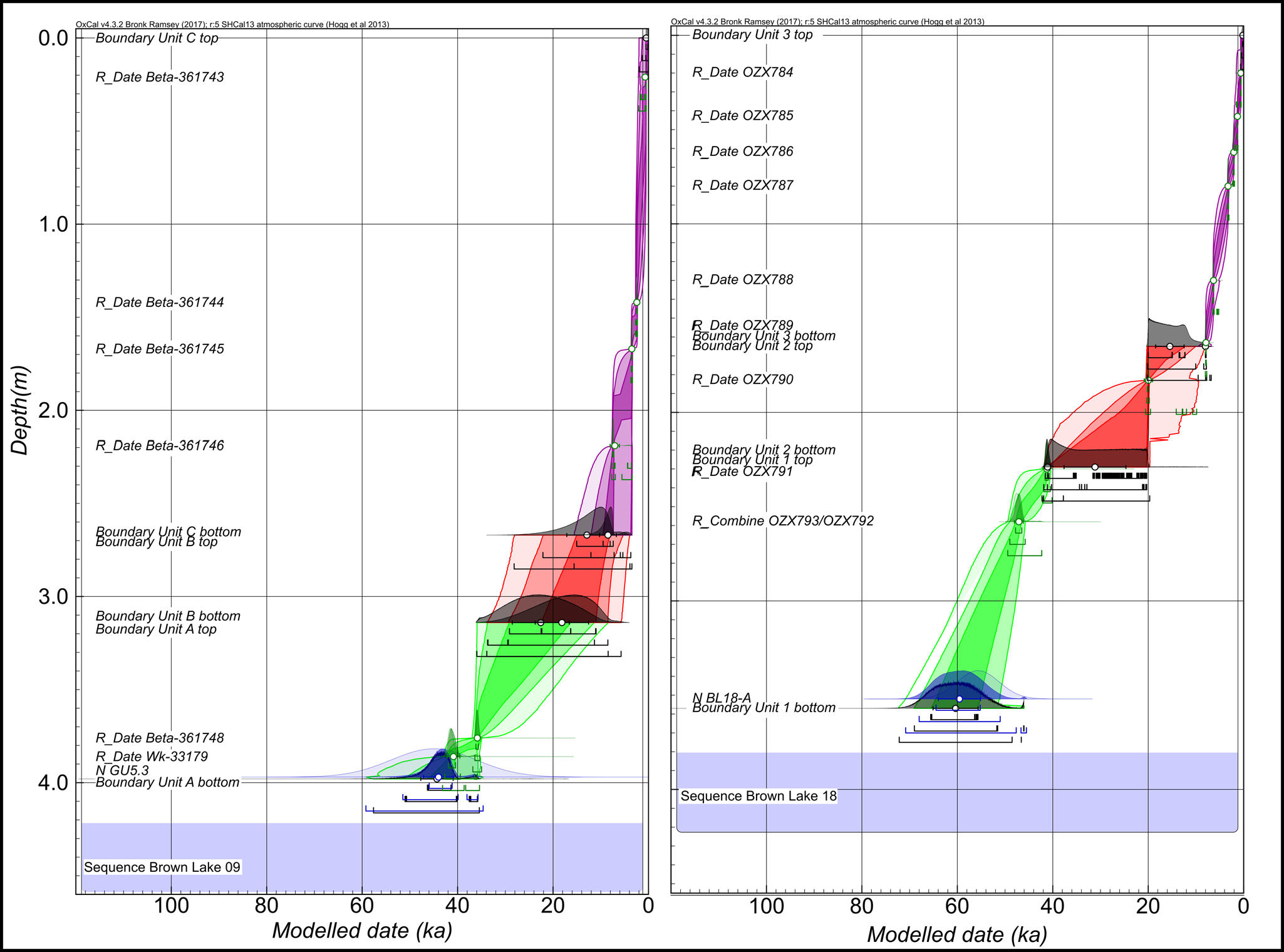
Figure 6. Bayesian age-depth model constructed in OxCal version 4.3.2 using the single-grain OSL and 14C ages obtained for the BL09 (left) and BL18 (right) cores. The original probability distributions for the OSL (blue) and 14C (green) age estimates (the likelihoods) and the posterior modeling distributions are represented as light and dark shading of the respective colors. The age-depth model envelopes show the 99%, 95%, and 68% highest probability density ranges for each of the main depositional units (green, red, and magenta), as identified by sedimentological analysis. The modeled posterior distributions for the unit boundaries are shown in grey. (For interpretation of the references to color in this figure legend, the reader is referred to the web version of this article.)
The BL18 and BL09 Bayesian models have agreement index (Amodel) values of 100.4% and 101.2%, respectively, and overall agreement index (Aoverall) values of 99.9% and 100.6%, respectively—all above the minimum threshold of 60% (Bronk Ramsey, Reference Bronk Ramsey2009). The outlier analysis of BL09 identified Beta-361743 as having a relatively high posterior probability of 22%. In core BL18, there were no samples that had exceptionally high posterior outlier probabilities (Fig. 6), with combined 14C samples OZX793/OZX792 identified as having low outlier probability of 8%. The modeled boundary ages and use of the OxCal Difference query (see Supplementary Information) show for the lowermost BL09 unit (Unit A) and equivalent BL18 unit (Unit 1) that deposition occurred between 44.3 ± 3.4–22.5 ± 6.0 ka and 60.4 ± 4.7–41.1 ± 0.6 ka, respectively. Deposition of the overlying units (BL09, Unit B; BL18, Unit 2) initiated ca. 18.1 ± 5.6 ka and 31.2 ± 6.5 ka, and ceased at 12.9 ± 4.2 ka and 15.5 ± 3.0 ka, respectively.
DISCUSSSION
North Stradbroke Island OSL dune ages
The majority of dune crest ages in this study—excluding NSI18-7, for which the timing is uncertain due to the complex distribution of the grain populations (Fig. 5)—corroborate previously inferred dune activation during MIS 5 on North Stradbroke Island (Pickett et al., Reference Pickett, Ku, Thompson, Roman, Kelley and Huang1989; Tejan-Kella et al., Reference Tejan-Kella, Chittleborough, Fitzpatrick, Thompson, Prescott and Hutton1990). Additionally, none of the final dune ages shown in Table 2 overlaps with the timing of the LGM (with the exception of the potentially compromised sample NSI18-7), suggesting limited mobilization of dune material at this time, despite increased aridity inferred from low lake levels (Figs. 7, 8).

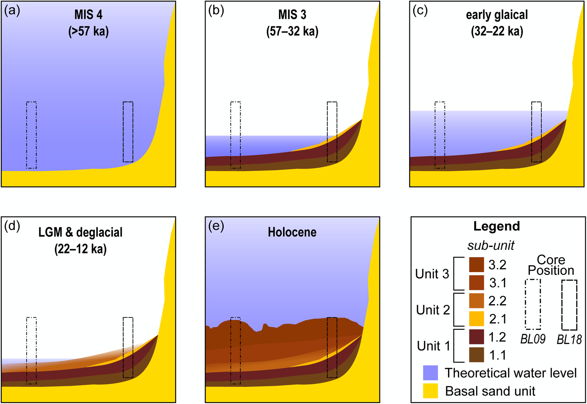
Figure 7. (color online) Conceptual model of sediment deposition and water level at Brown Lake during major climate phases referred to in text. The BL18 stratigraphic log was selected to represent the sedimentary units for the basin.

Figure 8. North Stradbroke Island wetland records with an extended range of inorganic sediment accumulation, and North Stradbroke Island dune crest ages over the last 160 ka. A global sea level curve is shown (Grant et al., Reference Grant, Rohling, Ramsey, Cheng, Edwards, Florindo, Heslop, Marra, Roberts and Tamisiea2014) (R.S.L.=relative sea level) along with the Brown Lake, Fern Gully Lagoon (Kemp et al., Reference Kemp, Tibby, Arnold, Barr, Gadd, Marshall, McGregor and Jacobsen2020), and Welsby Lagoon (Lewis et al., Reference Lewis, Tibby, Arnold, Barr, Marshall, McGregor, Gadd and Yokoyama2020) inorganic sediment accumulation records. The pink areas represent hiatus periods experienced at these wetlands. The red rectangle and arrow show the portion of the graph expanded in the bottom inset and identifies the change in mean accumulation rate between the wetland records. Dune OSL ages from this study (circles) are compared with those of Ellerton et al. (Reference Ellerton, Rittenour, Shulmeister, Gontz, Welsh and Patton2020) (squares) and Walker et al. (Reference Walker, Lees, Olley and Thompson2018) (triangles) from the Cooloola Sand Mass, with the timing of Yankee Jack dune building highlighted in yellow (Ellerton et al., Reference Ellerton, Rittenour, Shulmeister, Gontz, Welsh and Patton2020). (For interpretation of the references to color in this figure legend, the reader is referred to the web version of this article.)
The mean OSL age for the samples in this study excluding NSI17-7 is 119.9 ± 10.6 ka. Notably, this overlaps with the timing of the Yankee Jack unit emplacement reported (e.g., Ellerton et al., Reference Ellerton, Rittenour, Shulmeister, Gontz, Welsh and Patton2020) (Fig. 8) and supports the local distribution of the morphosequence as remapped using remote sensing (Patton et al., Reference Patton, Ellerton and Shulmeister2019) (Fig. 1b). The OSL results from this study show limited dune building during the LGM on North Stradbroke Island despite increased aridity, a similar finding to Fraser Island (da Silva and Shulmeister, Reference da Silva and Shulmeister2016) and across the Cooloola Sand Mass (Ellerton et al., Reference Ellerton, Rittenour, Shulmeister, Gontz, Welsh and Patton2020). There appears to be a link between dune emplacement and higher sea-levels during MIS 5 (Fig. 8). This finding is in agreement with dune activation mechanisms proposed in the south-east Australian dune fields (Lees, Reference Lees2006; Ellerton et al., Reference Ellerton, Rittenour, Shulmeister, Gontz, Welsh and Patton2020). Moreover, the absence of substantial evidence indicating Holocene activation suggests the sand dunes had stabilized soon after deposition. However, an increase in the spatial resolution of dune samples across North Stradbroke Island is required to fully assess this hypothesis.
Lacustrine sediment accumulation in wetlands within the Yankee Jack dune sequence did not initiate synchronously, based on our regional dating comparison (i.e., Fern Gully Lagoon = ca. 209 ka [Kemp et al., Reference Kemp, Tibby, Arnold, Barr, Gadd, Marshall, McGregor and Jacobsen2020]; Welsby Lagoon = ca. 83 ka [Lewis et al., Reference Lewis, Tibby, Arnold, Barr, Marshall, McGregor, Gadd and Yokoyama2020]; and Brown Lake = ca. 60 ka) (Fig. 8). This supports the notion that the formation of the respective perching layers is not dictated purely by the mineralogical composition of the Yankee Jack dune sequence. Rather, it was likely a combination of local catchment morphology and hydroclimate (cf., Brooke et al., Reference Brooke, Preda, Lee, Cox, Olley, Pietsch and Price2008).
Brown Lake BL09 and BL18 age models
The difference in sediment accumulation rate between the two Brown Lake records (Fig. 6) suggests that sedimentation was influenced by their position relative to water level (Fig. 7). The bathymetry of the modern lake-floor has a downwards slope trending in a north-east direction with an undulating surface (Fig. 2). During times of lower lake level, water turbulence in combination with the uneven surface may have changed the position of the fine-sediment accumulation zone (Blais and Kalff, Reference Blais and Kalff1995). This change in the sediment-focusing position would likely not affect the deposition of the sand band because this feature is likely accumulation of local material near the edge of the lake (Fig. 7); thus explaining why the distinctive sand band is observed in BL18 and not BL09.
The difference between the ages for the BL18 and BL09 records may also be grounded in the resolution of input parameters in the age model. The BL18 age-depth model has a resolution of more than three dating samples per meter (ten 14C samples, including one replicate from 258 cm, and one OSL sample), whereas BL09 has notably fewer (six 14C samples and one OSL sample) (Tables 1, 2). The proximity of the individual age estimates to the unit boundaries in each core also likely influences the age model outcomes. For example, the transition between Unit 2 and Unit 3 in BL18 is bracketed by 14C samples OZX790 and OZX789 (Table 1; Fig. 2), thereby increasing confidence that the depositional interval has been modeled accurately. In contrast, the same boundary transition in the BL09 core (i.e., Unit B and Unit C transition) is not as well constrained, and the modeled age for Unit B relies on interpolation between ages from underlying and overlying units (Table 1, Fig. 6). The disparity in ages observed between parts of the BL18 and BL09 cores highlights the need to understand basin morphology, and the importance of developing robust age models before drawing inferences from paleoenvironmental proxies.
History of aeolian sediment deposition in Brown Lake
The change and variability inferred from Brown Lake are based on the BL18 record, which has the better age-depth model. Reconstructing the broader evolution of the wetland, however, considers both BL18 and BL09 (Fig. 7) and draws on comparisons to other North Stradbroke Island records where variation in inorganic sediment geochemistry has been used to infer aeolian deposition (e.g., Petherick et al., Reference Petherick, McGowan and Moss2008; Moss et al., Reference Moss, Tibby, Petherick, McGowan and Barr2013; Kemp et al., Reference Kemp, Tibby, Arnold, Barr, Gadd, Marshall, McGregor and Jacobsen2020; Lewis et al., Reference Lewis, Tibby, Arnold, Barr, Marshall, McGregor, Gadd and Yokoyama2020). In this study, comparisons to Welsby Lagoon have utilized the alternate age-depth model presented in Lewis et al. (Reference Lewis, Tibby, Arnold, Barr, Marshall, McGregor, Gadd and Yokoyama2020, fig. S5B). The use of this alternate age model was preferred given the co-occurrence of hydrological change inferred in the Brown Lake and Fern Gully Lagoon records, the expression of which appears dampened in Welsby Lagoon due to its transition from a lake to a swamp (Cadd et al., Reference Cadd, Tibby, Barr, Tyler, Unger, Leng, Marshall, McGregor, Lewis and Arnold2018). Use of this alternative age model is acceptable because it was shown to be relatively insensitive to the choice of stratigraphic priors (Lewis et al., Reference Lewis, Tibby, Arnold, Barr, Marshall, McGregor, Gadd and Yokoyama2020). Moreover, interpretations of dust flux were considered with respect to increased atmospheric dust loads (Harrison et al., Reference Harrison, Kohfeld, Roelandt and Claquin2001), which in Australia resulted from reduced vegetation due to drier climate (Hesse and McTainsh, Reference Hesse and McTainsh2003; McGowan et al., Reference McGowan, Petherick and Kamber2008), changing wind direction or strength (Kohfeld et al., Reference Kohfeld, Graham, de Boer, Sime, Wolff, Le Quéré and Bopp2013), sediment recharge in dust-source areas (Farebrother et al., Reference Farebrother, Hesse, Chang and Jones2017), or a complex mix of all these variables in response to hydrological variation (Marx et al., Reference Marx, Kamber, McGowan, Petherick, McTainsh, Stromsoe, Hooper and May2018).
MIS 4 (>57 ka)
The mean modeled age for the base of Brown Lake (BL18) is 60.4 ± 4.7 ka (Fig. 6), though the perched indurated layer must have formed before this time. Prior to this study, the oldest date from Brown Lake (BL09) was 47.2 ka (Tibby et al., Reference Tibby, Barr, Marshall, McGregor, Moss, Arnold and Page2017). The early portion of the Brown Lake MIS 4 sedimentary record (Fig. 7a) likely accumulated during a phase of positive moisture balance with a lowered influx of aeolian material (Fig. 9) and lake-full conditions promoting substantial organic matter production and preservation (Fig. 7). The Fern Gully Lagoon record also has a low inorganic flux through MIS 4 (Kemp et al., Reference Kemp, Tibby, Arnold, Barr, Gadd, Marshall, McGregor and Jacobsen2020; Fig. 9), which may be related to increased vegetation cover. Because dust on North Stradbroke Island is sourced from the central Australian basins (Magee et al., Reference Magee, Miller, Spooner and Questiaux2004; Cohen et al., Reference Cohen, Jansen, Gliganic, Larsen, Nanson, May, Jones and Price2015; Miller et al., Reference Miller, Fogel, Magee and Gagan2016) during MIS 4, it is likely that the coeval decline in dust flux is linked to wetter conditions regionally—an inference that would support the increase in rainforest taxa in ODP820 offshore from north-east Queensland (Kershaw et al., Reference Kershaw, Van Der Kaars and Moss2003). However, inferring climate from changes in dust flux sourced far afield should be made with caution because moisture and vegetation are not the only variables influencing dust mobilization. Dust flux can be influenced by source area surface aerodynamics (Webb and Strong, Reference Webb and Strong2011) and sediment recharge (Marx et al., Reference Marx, Kamber, McGowan, Petherick, McTainsh, Stromsoe, Hooper and May2018). The inorganic flux to Brown Lake and North Stradbroke Island is likely influenced by widespread fluctuations in moisture across Australia (Farebrother et al., Reference Farebrother, Hesse, Chang and Jones2017), with an additional factor being changed vegetation regimes from deep-rooted trees and shrubs to grasses and herbs.

Figure 9. Compilation of dust and inorganic flux records from North Stradbroke Island and the ocean for the past 65 ka. Periods shown are modified from those identified in the OZ-INTIMATE climate synthesis (Reeves et al., Reference Reeves, Barrows, Cohen, Kiem, Bostock, Fitzsimmons, Jansen, Kemp, Krause and Petherick2013). The dust records shown include dust flux from Tortoise Lagoon, Native Companion Lagoon (Petherick et al., Reference Petherick, Moss and McGowan2011, Reference Petherick, Moss and McGowan2017), the South Pacific Ocean (Lamy et al., Reference Lamy, Gersonde, Winckler, Esper, Jaeschke, Kuhn, Ullermann, Martinez-Garcia, Lambert and Kilian2014), and Brown Lake. Relative sea level data from the Red Sea (Grant et al., Reference Grant, Rohling, Ramsey, Cheng, Edwards, Florindo, Heslop, Marra, Roberts and Tamisiea2014) are displayed in grey and overlain by composite sea-level record data (Lambeck et al., Reference Lambeck, Rouby, Purcell, Sun and Sambridge2014). The yellow shaded box represents a potentially eroded section containing mixture of non-lacustrine and aeolian material, as discussed in the text. (For interpretation of the references to color in this figure legend, the reader is referred to the web version of this article.)
MIS 3 (57–32 ka)
The Brown Lake MIS 3 record shows increasing variation in PC1, attributed to progressively increasing influx of inorganic windswept material into the basin relative to MIS 4 (Fig. 9) rather than a proportional decrease in organic production (Fig. 7a, b). This is particularly notable between ca. 54 and 41 ka (Fig. 9), with concurrent trends observed in the Welsby Lagoon and the Fern Gully Lagoon records. However, unlike Fern Gully Lagoon, where two peaks of inorganic deposition occur at ca. 54 ka and ca. 47 ka (Kemp et al., Reference Kemp, Tibby, Arnold, Barr, Gadd, Marshall, McGregor and Jacobsen2020), the Brown Lake record shows a gradual increase in aeolian deposition through MIS 3, suggesting the difference may be attributed to local factors such as variation in lake water surface area, current flow, or vegetation regime changes influencing dust transport into the wetlands (Cadd et al., Reference Cadd, Tibby, Barr, Tyler, Unger, Leng, Marshall, McGregor, Lewis and Arnold2018). The history of marginal dune vegetation is not as well established for Brown Lake, in contrast to some other North Stradbroke Island sites (e.g., Moss et al., Reference Moss, Tibby, Petherick, McGowan and Barr2013).
MIS 3 and early glacial period
Through MIS 3, Brown Lake experienced a phase of sustained negative moisture balance, subsequently leading to shoreline transgression and deposition of the sandy sub-unit 2.1 ca. 30.9 ka (Fig. 7). The extent to which fire was a factor in enhancing local sand transportation remains unclear because charcoal records from nearby Welsby Lagoon show limited evidence for increased activity between MIS 4 and MIS 3 (Cadd et al., Reference Cadd, Tyler, Tibby, Baldock, Hawke, Barr and Leng2020). Moreover, owing to the lack of structure in the black muds (Unit 1) of Brown Lake, it is difficult to determine whether disruption occurred during the emplacement of the sandy sub-unit 2.1. Additionally, when considering the spatial variability factors such as fires and surface roughness have on sediment erosion (Sankey et al., Reference Sankey, Eitel, Glenn, Germino and Vierling2011), it is unreasonable to exclude deposition of the sand layer as occurring as part of a rapid event (e.g., storm activity). Nevertheless, there is a relationship between the increase in dust flux to Brown Lake (Fig. 9) and lower lake water levels, indicating negative moisture balance locally.
Wetlands nearby Brown Lake, (i.e., Fern Gully Lagoon and Welsby Lagoon records) also show a hiatus in late MIS 3 (Figs. 8, 9) and support lower precipitation. This is contrary to the Tortoise Lagoon and Native Cosmpanion Lagoon records, which continue to accumulate dust through this phase, although at a decreased rate (McGowan et al., Reference McGowan, Petherick and Kamber2008; Petherick et al., Reference Petherick, McGowan and Moss2008; Petherick et al., Reference Petherick, Moss and McGowan2017), and generally support a regional shift towards warm and wet conditions; as suggested by pollen records (Moss et al., Reference Moss, Tibby, Petherick, McGowan and Barr2013). The disparity between these sites may be attributed to contrasting local catchment conditions and morphologies, which may have altered sediment infilling dynamics (e.g., Fern Gully Lagoon and Welsby Lagoon), shoreline migrations (e.g., Brown Lake), establishment of denser vegetation communities in close proximity (e.g., Tortoise Lagoon and Native Companion Lagoon), or a combination of these factors. Given age models show breaks in the Brown Lake, Fern Gully, and Welsby Lagoon cores are coeval, the cause of which is considered to be a result of more arid conditions attributed to changes in the relative positioning and strength of ENSO (Merkel et al., Reference Merkel, Prange and Schulz2010) and key rainfall bands across the Pacific Ocean—as shown in modern interannual climate models (Brown et al., Reference Brown, Lengaigne, Lintner, Widlansky, Van Der Wiel, Dutheil, Linsley, Matthews and Renwick2020). Therefore, the suppression of rainfall across the Brown Lake catchment during glacial times would cause water level to fall and shorelines to regress. Moreover, reduced evaporation from lowered temperatures may have prevented the lake drying completely as reported in nearby wetlands (Cadd et al., Reference Cadd, Tibby, Barr, Tyler, Unger, Leng, Marshall, McGregor, Lewis and Arnold2018). However, as presented in the age model results and supporting information, the choice of age model may affect the interpretation of lake evolution. As glacial conditions began to weaken North Atlantic meridional overturning circulation, thus modifying ENSO once more, changing local precipitation patterns and the strength of winds carrying continentally sourced dust to North Stradbroke Island (e.g., Harrison, Reference Harrison1993; Petherick et al., Reference Petherick, McGowan and Moss2008). This ultimately drove the changes in lake water levels for wetlands, particularly Brown Lake, and allowed them to persist through MIS 2 (Figure 7c-d).
Last glacial maximum (22–18 ka)
The Brown Lake, Fern Gully Lagoon, and Welsby Lagoon sediment records show that there has been a pause in, or erosion of, lacustrine deposition leading into the LGM (Fig. 9). The difference between these records, despite their relatively close proximity (<8 km; Fig. 1), may reflect local variations in conditions favoring expansion of the indurating layer (Brooke et al., Reference Brooke, Preda, Lee, Cox, Olley, Pietsch and Price2008), subsequently leaving wetlands with smaller perched aquifer catchments more susceptible to water level decline and shoreline regression during periods of moisture stress. Additionally, differences between the wetlands at this time (e.g., Welsby Lagoon transitioning into a swamp; Cadd et al., Reference Cadd, Tibby, Barr, Tyler, Unger, Leng, Marshall, McGregor, Lewis and Arnold2018) may have limited their ability to accumulate aeolian material. The various morphological changes that these wetlands can experience have profound influences on how records may be interpreted, highlighting the need establish thoroughly dated records in order reliably compare to regional archives of an early glacial change.
The Brown Lake record shows that dust deposition was highest through the early glacial and LGM phases, peaking at ca. 23 ka (Fig. 9), a timing comparable to peaks observed in the Native Companion Lagoon (Petherick et al., Reference Petherick, McGowan and Moss2008) and Tortoise Lagoon (Petherick et al., Reference Petherick, Moss and McGowan2017). Considered together, the agreement between these North Stradbroke Island wetlands could indicate a localized signal attributed to dune destabilization from vegetation burning and enhanced dust mobilization, although there is limited change in the charcoal record (Cadd et al., Reference Cadd, Tyler, Tibby, Baldock, Hawke, Barr and Leng2020). A similar dust record is reflect in South Pacific Ocean marine cores (De Deckker, Reference De Deckker2001; Lamy et al., Reference Lamy, Gersonde, Winckler, Esper, Jaeschke, Kuhn, Ullermann, Martinez-Garcia, Lambert and Kilian2014), where it is suggested dust generation was a result of regional climatic change. Thus, it can be inferred that the Brown Lake record hosts information related to the increased supply, entrainment, and transport of material from regional dust sources (Marx et al., Reference Marx, Kamber, McGowan, Petherick, McTainsh, Stromsoe, Hooper and May2018), the deflation of which was enhanced by drier conditions associated with the early glacial period and into the LGM. Moreover, the dust transportation pathways (Petherick et al., Reference Petherick, McGowan and Kamber2009) show the source of the inorganic material was far-travelled, originating from the Australian mainland, where dust generation was linked to changes in moisture balance (Hesse and McTainsh, Reference Hesse and McTainsh2003). Movement of the South Pacific Convergence Zone and the on-flowing effect to how ENSO is expressed have the capacity to influence generally drier conditions, including enhancement of the SW winds, through displacement and suppression of other synoptic fronts on the east coast (Rudeva et al., Reference Rudeva, Simmonds, Crock and Boschat2019; Brown et al., Reference Brown, Lengaigne, Lintner, Widlansky, Van Der Wiel, Dutheil, Linsley, Matthews and Renwick2020).
The modeled mean accumulation rate for Brown Lake through the LGM (0.04 m/ka) was surprisingly lower than MIS 3 (0.06 m/ka) (Fig. 8), although this may reflect limited age-model precision between Unit 2 and Unit 1. Therefore, the Brown Lake data should be expected to be in agreement with Fern Gully Lagoon and Welsby Lagoon, which show accumulation rates increasing from 0.01 m/ka to 0.08 m/ka (Kemp et al., Reference Kemp, Tibby, Arnold, Barr, Gadd, Marshall, McGregor and Jacobsen2020) and 0.17 m/ka to 0.23 m/ka (Lewis et al., Reference Lewis, Tibby, Arnold, Barr, Marshall, McGregor, Gadd and Yokoyama2020), respectively (Fig. 8). Furthermore, an increase in lithogenic material accumulation would correlate with increased atmospheric dust loads (Harrison et al., Reference Harrison, Kohfeld, Roelandt and Claquin2001), which likely resulted from drier climate, albeit modulated by other factors.
The variation in chemical composition in the Brown Lake record for the early glacial phase and LGM (i.e., the clays of Unit 2) supports the hypothesis that dust was being sourced outside of North Stradbroke Island (Petherick et al., Reference Petherick, McGowan and Kamber2009). Moreover, the sedimentological properties of sub-unit 2.2 suggest that the Brown Lake water level fluctuated soon after the LGM, falling below the sediment surface between 15.4 ± 3.1 ka (top of Unit 2) and 8.0 ± 0.2 ka (bottom of Unit 3) (Fig. 7c, d). The timing of this break in sedimentation is different from other North Stradbroke Island wetlands (Fig. 9) and may be a product of different conditions between each catchment, or their respective age models. Nevertheless, the mechanism influencing precipitation across the catchments is likely regional, possibly linked to the Antarctic Cold Reversal (Barr et al., Reference Barr, Tibby, Moss, Halverson, Marshall, McGregor and Stirling2017), or ENSO because geographically separate climate records across the Australian continent also indicate a change towards more positive moisture balance during the deglacial phase (Turney et al., Reference Turney, Kershaw, James, Branch, Cowley, Fifield, Jacobsen and Moss2006b; Williams et al., Reference Williams, Cook, van der Kaars, Barrows, Shulmeister and Kershaw2009; Petherick et al., Reference Petherick, Bostock, Cohen, Fitzsimmons, Tibby, Fletcher, Moss, Reeves, Mooney and Barrows2013).
The Holocene (11.7–0 ka)
Following the depositional hiatus at Brown Lake during the deglacial period, a return to higher lake levels, according to our model, occurred ca. 8 ka and allowed aeolian inorganic material to accumulate once again. Notably, the timing of the hiatus is in agreement with drier conditions observed in Lake Allom from the nearby Fraser Island (Donders et al., Reference Donders, Wagner and Visscher2006). Because the increase in lake water level is coeval between two separate lakes, it is more likely this reflects a regional increase in moisture across eastern Australia, the timing of which aligns with enhancement of Southern Hemisphere circulation (Woodward et al., Reference Woodward, Shulmeister, Bell, Haworth, Jacobsen and Zawadzki2014). The Brown Lake, Welsby Lagoon, and Fern Gully Lagoon records have contrasting Holocene dust flux, with Brown Lake showing a declining PC1 signal, Welsby Lagoon relatively stable (Lewis et al., Reference Lewis, Tibby, Arnold, Barr, Marshall, McGregor, Gadd and Yokoyama2020), and Fern Gully Lagoon showing an increasing flux (Kemp et al., Reference Kemp, Tibby, Arnold, Barr, Gadd, Marshall, McGregor and Jacobsen2020) (Fig. 9). The variance between the records may be linked to differing hydrological sensitivities, chronological model frameworks, or other site-specific factors (Cadd et al., Reference Cadd, Tibby, Barr, Tyler, Unger, Leng, Marshall, McGregor, Lewis and Arnold2018) Conversely, following the hiatus at Brown Lake, the basin returned to a deeper lacustrine system similar to its expression today (Fig. 7e). Elsewhere, the smaller catchment size of Fern Gully Lagoon relative to other North Stradbroke Island wetlands (Kemp et al., Reference Kemp, Tibby, Arnold, Barr, Gadd, Marshall, McGregor and Jacobsen2020) appears to have increased the wetland's susceptibility to drying out during periods of lower rainfall on the island (Barr et al., Reference Barr, Tibby, Leng, Tyler, Henderson, Overpeck and Simpson2019).
Differing human land-use practices may also be a factor in the different signals observed in the wetland records. Increased burning may have induced changes in vegetation cover (Barr et al., Reference Barr, Tibby, Moss, Halverson, Marshall, McGregor and Stirling2017; Mariani et al., Reference Mariani, Tibby, Barr, Moss, Marshall and McGregor2019), thereby altering the erosivity of the soil. However, information pertaining to human occupation on North Stradbroke Island is limited, with late Pleistocene archaeological evidence from Wallen Wallen Creek providing the earliest known activity (ca. 20,560 ± 250 14C yr BP [SUA-2341]; Neal and Stock, Reference Neal and Stock1986).
CONCLUSION
Single-grain OSL ages obtained on dune crests in this study indicate activation of the Yankee Jack dune sequence on North Stradbroke Island through MIS 5, the earliest initiation being 167.8 ± 19.1 ka. Subsequent to this prominent phase of dune building, there was long-term stabilization of the local dune landscape with no indication of subsequent large-scale dune mobilization. This may be attributed to vegetation stabilizing the MIS 5 age dunes of North Stradbroke Island shortly after emplacement by 91.0 ± 9.1ka.
The new paleoenvironmental record from Brown Lake, which includes a Bayesian age depth model derived from 10 14C ages and an OSL date, has enabled inference of climate variability over the past 60 ka. Geochemical and sedimentological changes, driven by changes in dust deposition, highlight the sensitivity of this perched wetland to climate change. The age model suggests the sedimentary sequence is continuous from lake initiation to the LGM. However, the sedimentology at the base of Unit 2 may indicate dry lake conditions or rapid sand deposition; further chronological control through this part of the record is required to differentiate between these scenarios. Nevertheless, from late MIS 3 and MIS 2 the dust flux signal intensifies across North Stradbroke Island, the result of which aligns with continental aridification and ecological change across Australia.
The increase in dust deposition across Brown Lake, Tortoise Lagoon, and Native Companion Lagoon during the early glacial phase and LGM, and the coeval hiatuses between Brown Lake and nearby wetlands, support a climate-driven local expression of negative moisture balance. This contrasts with interferences of a largely positive moisture balance at this time (e.g., Moss et al., Reference Moss, Tibby, Petherick, McGowan and Barr2013; Tibby et al., Reference Tibby, Barr, Marshall, McGregor, Moss, Arnold and Page2017), however it should be noted these have relatively fewer dates incorporated into the respective age models. Hence there is a need for better chronological controls so that local and regional changes can be evaluated. The inferred negative hydrological period in this study is in agreement with other terrestrial records across mainland Australia and New Zealand, potentially linked to changes in the positioning of the South Pacific Convergence Zone (Brown et al., Reference Brown, Lengaigne, Lintner, Widlansky, Van Der Wiel, Dutheil, Linsley, Matthews and Renwick2020), ENSO (Merkel et al., Reference Merkel, Prange and Schulz2010), South Westerly Winds (Rudeva et al., Reference Rudeva, Simmonds, Crock and Boschat2019), or a combination thereof. Comparisons of Brown Lake to proximal wetlands through MIS 2 in particular (i.e., Welsby Lagoon and Fern Gully Lagoon) have highlighted the importance of understanding variations in local catchment ecology and morphology, particularly when considering the impact of basin infilling on paleoenvironmental records.
The return to a more positive moisture balance at Brown Lake in the early Holocene, and the recommencement of sediment accumulation, suggests a local shift from dry to wet. However, interrogating the dust record alone for regional changes in climate following recommencement is less reliable because landscape alteration from human practices both locally and in source locations had likely initiated. In order to better understand the effects of climate variation on the environment, particularly in association with the LGM and climate extremes, multi-proxy analytical approaches should also consider the surrounding landscape (e.g., associated dune deposits), which may hold missing or complementary information about local variations in environmental conditions.
ACKNOWLEDGMENTS
We acknowledge Minjerribah (North Stradbroke Island) and the surrounding waters as Quandamooka Country and thank the Quandamooka Yoolooburrabee Aboriginal Corporation for permission to undertake the work. We thank Haidee Cadd and Jo Blessing for assistance in the field and Chris Kemp for discussions pertaining to Fern Gully Lagoon. Many thanks are also extended to Jonathan Marshall and Glenn McGregor for assistance in data acquisition. The work was supported by the Australian Research Council Discovery Project (DP150103875). R.L. was supported by an Australian Government Research Training Program Scholarship and a CRC LEME Regolith Science Scholarship. The OSL dating was supported by Australian Research Council Future Fellowship (FT130100195). Radiocarbon dating and XRF core scanning was made possible through the ANSTO facility access program (AP11643; AP12402). We acknowledge the financial support from the Australian Government for the Centre for Accelerator Science at ANSTO through the National Collaborative Research Infrastructure Strategy (NCRIS).
SUPPLEMENTARY MATERIAL
The supplementary material for this article can be found at https://doi.org/10.1017/qua.2020.117