


Introduction
Most of the circum-Arctic lands were marked by human occupation for millennia, even the Canadian Arctic and northern Greenland where early settlements of pre-Inuit date from about 4000 yr (e.g., Raghavan et al., Reference Raghavan, DeGiorgio, Albrechtsen, Moltke, Skoglund, Korneliussen and Grønnow2014). However, Svalbard apparently remained free of human occupation until historical times (Arlov, Reference Arlov2005). Artifacts dating from the Stone Age were tentatively attributed by Christiansson and Simonsen (Reference Christiansson and Simonsen1970) to early settlements, but the nature of the artifacts was questioned, and the evidence denied by some archaeologists (e.g., Bjerk, Reference Bjerk2000). Norsemen and Russian Pomors possibly made early stays in Svalbard by the end of the Middle Age but the first unquestioned settlements in Svalbard date from the late sixteenth century, when whalers and hunters from northwest European started to exploit the Svarbard coastal regions, at least seasonally (Albrethsen and Arlov, Reference Albrethsen and Arlov1988; Arlov, Reference Arlov2005). Whereas harsh climate and low marine productivity that would have sustained and/or attracted human populations could explain the late arrival of humans on Svalbard, little is known about climate and surface ocean conditions prior to the instrumental period, especially in the northeast, where the coast lines are bathed by the Barents Sea and Arctic Ocean waters. Here, we document postglacial sea-surface conditions off northeast Svalbard based on the palynological content of a core collected in Kvitøya Trough (Fig. 1) in the northern Barents Sea, which is the second main gateway between the Atlantic and Arctic oceans after Fram Strait (Årthun et al., Reference Årthun, Eldevik, Smedsrud, Skagseth and Ingvaldsen2012). Hence, the northern Barents Sea that makes the transition from Atlantic to Arctic waters is a region that might have experienced important climate changes.
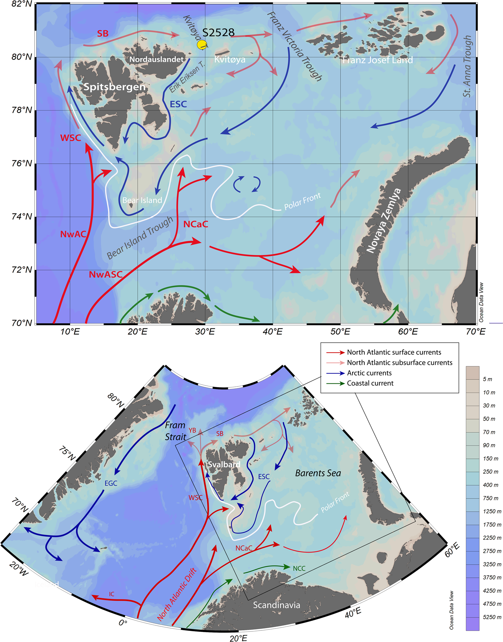
Figure 1. Maps showing the location of core S2528 and modern surface currents in the Barents Sea. The red arrows illustrate the circulation pattern of Atlantic waters at the surface, including the Norwegian Atlantic Current (NwAC) and the Norwegian Atlantic Slope Current (NwASC), which divides into the West Spitsbergen Current (WSC) and the North Cape Current (NCC). North of Svalbard, the WSC becomes the subsurface current of the Svalbard Branch (SB) and the Yermak Branch (YB). The blue arrows show the Arctic East Spitsbergen Current (ESC) and East Greenland Current (EGC). The green arrows correspond to coastal currents. The polar front position is represented by the white line based on Loeng (Reference Loeng1991).
The inflow of Atlantic water northeastward through the Barents Sea Opening presently represents a mean flux of 2.3 Sv and constitutes an important source of heat in the Barents Sea, with an annual average of 49 TW as recorded between 1998 and 2008 (Årthun et al., Reference Årthun, Eldevik, Smedsrud, Skagseth and Ingvaldsen2012). Because Atlantic water loses most of its heat content in the Barents Sea (Årthun and Schrum, Reference Årthun and Schrum2010), remaining heat transport through the northern exit is relatively small (Gammelsrød et al., Reference Gammelsrød, Leikvin, Lien, Budgell, Loeng and Maslowski2009). In the Barents Sea, the polar front position at the winter limit of sea-ice cover extent is highly sensitive to variations in heat advected from the North Atlantic Ocean. The northwestern Barents Sea is therefore located in the center of action for what concerns exchanges between cold surface waters from the Arctic Ocean and the northernmost branches of the relatively warm North Atlantic water. In the Barents Sea, any change in Atlantic current intensity may impact the distribution of sea ice (Årthun et al., Reference Årthun, Eldevik, Smedsrud, Skagseth and Ingvaldsen2012) and ocean-atmosphere heat exchanges, thus playing an important role in regional climate and accounting for a part of the overall strength of the Atlantic Meridional Overturning circulation (AMOC; Rudels et al., Reference Rudels, Anderson and Jones1996; Dieckmann and Hellmer, Reference Dieckmann, Hellmer, Thomas and Dieckmann2008; Smedsrud et al., Reference Smedsrud, Esau, Ingvaldsen, Eldevik, Haugan, Li and Lien2013).
With the aim of reconstructing sea-surface conditions since the deglaciation and their relationship with variations in the relative flow of North Atlantic water into the Barents Sea, we analyzed the palynological content of a marine sediment core (S2528) collected in Kvitøya Trough in the northwestern part of the Barents Sea (Fig. 1). Among palynological tracers, assemblages of dinoflagellate cysts (hereafter dinocysts) deserve special attention. Dinoflagellates are unicellular organisms that include heterotrophic, phototrophic, and mixotrophic taxa (e.g., Jeong et al., Reference Jeong, Yoo, Kim, Seong, Kang and Kim2010), thus allowing to characterize productivity in the upper part of the water column. During their life cycle, in relation with their sexual reproduction, about 10–12% of the species form a cyst composed of refractory organic matter that fossilizes in sediment (e.g., Head, Reference Head, Jansonius and McGregor1996). The dinocyst fluxes to the sea floor yield a fragmentary picture of biological productivity in surface waters and their assemblage composition provide information on oceanographic conditions, including sea-surface temperature and salinity, seasonal sea-ice cover, and productivity (Rochon et al., Reference Rochon, de Vernal, Turon, Matthiessen and Head1999; de Vernal et al., Reference de Vernal, Henry, Matthiessen, Mudie, Rochon, Boessenkool and Eynaud2001, Reference de Vernal, Rochon, Fréchette, Henry, Radi and Solignac2013a, Reference de Vernal, Hillaire-Marcel, Rochon, Fréchette, Henry, Solignac and Bonnet2013b, Reference de Vernal, Radi, Zaragosi, Van Nieuwenhove, Rochon, Allan and De Schepper2019; Radi and de Vernal, Reference Radi and de Vernal2008). In this paper, we used dinocyst data to estimate conditions steered by the northward flow of Atlantic waters at the surface. Although the study core site is located offshore, far from potential human settlements, it provides insights into climate and marine environmental conditions for the northeast Svalbard region over the last millennia.
GEOGRAPHIC AND OCEANOGRAPHIC SETTING
The Barents Sea is a relatively shallow, continental shelf sea with a mean water depth of 230 m. Surface waters in the Barents Sea consist of three main water masses: the Coastal Water, the North Atlantic Water (NAW), and the Arctic Water (Fig. 2; Loeng Reference Loeng1991). The NAW is characterized by salinities higher than 35.0 psu. Between Norway and Bear Island, where the NAW remains close to the surface, sea-surface temperature (SST) ranges from 3.5 to 6.5°C in summer (Fig. 2). Both temperature and salinity decrease northeastward. The Coastal Water, formed from the mixing of North Atlantic water and terrestrial freshwater inputs (Sætre and Ljøen, Reference Sætre and Ljøen1972), has almost the same temperature as the NAW, but its salinity is lower than 34.7 psu. The Arctic Water originates from the north and is characterized by low salinity (34.3–34.8 psu) and SST below 0°C. During winter, in the northern part of the Barents Sea, the Arctic Water occupies the upper 150 m of the water column, while meltwater may result in a low-salinity (31–34.2 psu) surface-water layer 5–20 m thick in summer (Helland-Hansen and Nansen, Reference Helland-Hansen and Nansen1909). The NAW layer occupies most of the water column in the southern Barents Sea (Risebrobakken et al., Reference Risebrobakken, Moros, Ivanova, Chistyakova and Rosenberg2010, Reference Risebrobakken, Dokken, Smedsrud, Andersson, Jansen, Moros and Ivanova2011), but it lies mostly at depths between 120 and 200 m in the northern Barents Sea (Duplessy et al., Reference Duplessy, Ivanova, Murdmaa, Paterne and Labeyrie2001).

Figure 2. Map of mean summer (a) sea-surface temperature and (b) salinity over the Barents Sea between 1955 and 2012, after the World Ocean Atlas (Locarinini et al., Reference Locarnini, Mishonov, Antonov, Boyer, Garcia, Baranova and Zweng2013; Zweng et al., Reference Zweng, Reagan, Antonov, Locarnini, Mishonov, Boyer and Garcia2013). The white dashed lines separate the North Atlantic waters (NAW), the Arctic waters (ArcW) and the Coastal waters (CW), as defined by Loeng (Reference Loeng1991).
The North Cape Current, a North Atlantic branch flowing along the Scandinavian coasts, transports most of the heat to the Barents Sea through the Bear Island Trough (Fig. 1). It controls the polar front position at the sea-ice limit (Loeng, Reference Loeng1991). The inflow of the North Cape Current mainly follows a counterclockwise trajectory before exiting the Barents Sea between Novaya Zemlya and Franz Josef Land (Schauer et al., Reference Schauer, Loeng, Rudels, Ozhigin and Dieck2002). Relatively warm (+0.5 to 1°C) and saline (34.7–35.1 psu) modified Atlantic water subducting in Fram Strait spreads as a subsurface current along the continental slope of the Nansen Basin and enters the Barents Sea from the north via the relatively deep (400–600 m) Kvitøya and Franz Victoria Troughs, and in the Kara Sea via the St. Anna Trough (Lind and Invaldsen, Reference Lind and Ingvaldsen2012).
The surface water at our study site is presently under the dominant influence of the Arctic Water with SST <0°C and salinity between 34.3 and 34.7 psu in summer (Fig. 2; Pfirman et al., Reference Pfirman, Bauch, Gammelsrød, Johannessen, Muench and Overland1994). The Arctic Water is carried into the Barents Sea with the East Spitsbergen Current in the Franz Victoria and Kvitøya troughs, from where it flows south and west along the eastern Svalbard coast. Conductivity, temperature and density data show that the Arctic Water occupies the upper 50 m of the water column in the coring site area, with fresher water at the top (Ivanova et al., Reference Ivanova, Murdmaa, de Vernal, Risebrobakken, Peyve, Brice, Seitkalieva and Pisarev2019). Below 50 m, the subsurface to intermediate layer of the water column is occupied by the Atlantic-derived water coming from the Svalbard Branch that flows into the Kvitøya Trough from the northwest (Pfirman et al., Reference Pfirman, Bauch, Gammelsrød, Johannessen, Muench and Overland1994).
METHODS
Sediment core and chronology
The 385-cm-long sediment core S2528 (80°40.80′N; 29°36.70′E) was retrieved at a depth of 428 m in the Kvitøya Trough, between Nordaustlandet and the Kvitøya islands during Cruise 25 of R/V Akademik Nikolaj Strakhov in 2007.
The chronology of S2528 was established from accelerator mass spectrometry (AMS) 14C dates of mixed benthic foraminifers and bivalve shells collected in sediment slices of 3 cm or more in order to obtain enough material (Table 1). The AMS 14C dates are reported using the Libby half-life of 5568 yr and calibrated using the Marine13 calibration curve (Reimer et al., Reference Reimer, Bard, Bayliss, Beck, Blackwell, Bronk Ramsey and Buck2013). An additional correction (ΔR) of 71 ± 21 yr was used to account for the air–sea reservoir difference in the Barents Sea (Mangerud et al., Reference Mangerud, Bondevik, Gulliksen, Hufthammer and Høisæter2006). To create a chronological framework, we used Bacon (Blaauw and Christen, Reference Blaauw and Christen2011) and Clam (Blaauw, Reference Blaauw2010) software, both run in R. Bacon relies on a Bayesian approach and applies a high number of iterations for creating the “best model” within a confidence interval. The Clam software is simpler than Bacon but provides the option to define the type of interpolation and presents the advantage of allowing the sample thickness to be included. Because of the sparse dated intervals and because thick samples had to be sieved to collect enough biogenic carbonate for dating, we first applied Clam for interpolation and we developed the final age model with Bacon for calculating the confidence intervals or uncertainties.
Table 1. 14C dates of core S2528 and corresponding calibrated ages (Ivanova et al. [2019] with additions). Laboratory codes: Poz, Poznań Radiocarbon Laboratory; OS, NOSAMS facility at the Woods Hole Oceanographic Institution; CAMS, Lawrence Livermore National Laboratory.

Palynological analysis
Sediments from core S2528 were subsampled over 3 cm at 3-cm intervals for palynological analysis. Each 3-cm-thick sample was processed according to a standardized protocol (de Vernal et al., Reference de Vernal, Bilodeau and Henry2010). In brief, 1.5 to 5.0 cm3 was weighted and sieved at 106 and 10 μm. The dried fraction >106 μm, mainly composed of detrital material, was weighed and used as a proxy for ice rafting deposition and for hand-picking of foraminifers and other biogenic remains. The fraction between 10 and 106 μm was used for palynological preparations, which consisted in chemical treatment with room temperature HCl (10%) and HF (49%) to dissolve carbonate and silica particles. The residue was concentrated on a 10-μm nylon mesh and mounted on microscope slides with glycerol gelatin. Prior to the chemical treatment, Lycopodium clavatum spore tablets were added to the samples to allow estimating palynomorph concentrations (e.g., Mertens et al., Reference Mertens, Verhoeven, Verleye, Louwye, Amorim, Ribeiro and Deaf2009).
The palynological analysis was conducted by identifying and counting common palynomorphs, including contemporaneous and reworked pollen grains, spores, and dinocysts, Halodinium and other acritarchs, and foraminifer organic linings, with an optical microscope in transmitted light at magnifications of 400 × to 1000 × . A minimum of 300 dinocysts were identified and counted in most sample using the nomenclature summarized in Rochon et al. (Reference Rochon, de Vernal, Turon, Matthiessen and Head1999) and Radi et al. (Reference Radi, Bonnet, Cormier, de Vernal, Durantou, Faubert, Head, Henry, Pospelova, Rochon and Van Nieuwenhove2013). Relative abundance of dinocyst taxa was expressed as percentages versus counted dinocysts. Pollen grains and spores were counted to quantify inputs from land vegetation, using identification keys (e.g., McAndrews et al., Reference McAndrews, Berti and Norris1973). Reworked palynomorphs were counted as indicators of past sediment erosion, subsequent transport, and resedimentation. The concentration of palynomorphs was expressed as the number of specimens per cm3 of wet sediment. Palynomorph concentrations and dinocyst percentage data are presented in Supplementary Tables 1a and 1b.
Special attention was paid to the dinocyst data. Multivariate analyses using CANOCO 5 software (ter Braak and Smilauer, Reference ter Braak and Smilauer2012) were performed to quantitatively describe the assemblage. We used the modern analogue technique (MAT; Guiot and de Vernal, Reference Guiot and de Vernal2007) to quantitatively reconstruct the sea-surface conditions. In paleoceanography, the analogue approach is commonly used for quantitative estimation of past SST (Guiot and de Vernal, Reference Guiot and de Vernal2007). In the case of dinocyst assemblages for which we have developed a very large reference database (de Vernal et al., Reference de Vernal, Rochon, Fréchette, Henry, Radi and Solignac2013a, Reference de Vernal, Radi, Zaragosi, Van Nieuwenhove, Rochon, Allan and De Schepper2020), it is the preferred technique because it relies on similarities between fossil and modern assemblages and does not assume linear or unimodal relationships for calibrations based on regression. Moreover, because dinocyst assemblages depend upon temperature in addition to salinity, sea-ice cover, and trophic level, the MAT has the advantage of allowing simultaneous reconstruction of many parameters. Furthermore, MAT is appropriate in the present case since the reference database used here (n = 1492) includes a large number of data points in the polar and subpolar domains with a wide range of hydrographical conditions regarding salinity, sea-ice cover and temperatures (de Vernal et al., Reference de Vernal, Rochon, Fréchette, Henry, Radi and Solignac2013a, Reference de Vernal, Hillaire-Marcel, Rochon, Fréchette, Henry, Solignac and Bonnet2013b).
The parameters we reconstruct here include SST and °C in winter and summer, sea-surface salinity (SSS, psu) in winter and summer, sea-ice cover (months/yr > 50%) and primary productivity (gC/m2/yr). These parameters show a wide range of combinations in the reference database and explain the distribution of dinocyst assemblages as it was shown from canonical correspondence analyses (Radi and de Vernal, Reference Radi and de Vernal2008; de Vernal et al., Reference de Vernal, Rochon, Fréchette, Henry, Radi and Solignac2013a). The estimates are made from the standardized reference database of the Northern Hemisphere that includes 1492 reference sites and 66 taxa (http://www.geotop.ca; de Vernal et al., Reference de Vernal, Rochon, Fréchette, Henry, Radi and Solignac2013a). Reconstructions were made from the five best modern analogue sites found by the calculation of the distance (inversely proportional to the similarity) after log-transformation of percentage data, in order to give more weight to accompanying taxa that often have narrower ecological affinities than dominant taxa (e.g., de Vernal et al., Reference de Vernal, Henry, Matthiessen, Mudie, Rochon, Boessenkool and Eynaud2001). In the case of the n = 1492 database, the threshold distance for good analogues is 1.2. Modern oceanographical values at the five selected modern analogue sites were used to define the maximum and minimum possible and the most probable value, which corresponds to the average weighted inversely to the distance.
The validation tests to evaluate the accuracy of the approach indicated that the root mean square errors of prediction are ± 1.4 months/yr for the sea-ice cover, ±1.1°C and ±1.6°C for winter and summer SSTs, ±2.6 psu for summer SSS, and ± 55 gC/m2 for productivity (de Vernal et al., Reference de Vernal, Rochon, Fréchette, Henry, Radi and Solignac2013a). MAT has been criticized because it possibly underestimates the error of prediction due to spatial autocorrelation (Telford, Reference Telford2006; Telford and Birks, Reference Telford and Birks2009). However, different tests performed to overcome the effect of spatial autocorrelation illustrate that the performance of MAT are comparable or better than those of transfer function techniques (Guiot and de Vernal, Reference Guiot and de Vernal2011; Hohmann et al., Reference Hohmann, Kucera and de Vernal2020).
In order to assess the reliability of estimates beyond the error of prediction, a reliability index can be calculated, as proposed by de Vernal et al. (Reference de Vernal, Hillaire-Marcel and Darby2005, Reference de Vernal, Hillaire-Marcel, Rochon, Fréchette, Henry, Solignac and Bonnet2013b). The index takes into consideration the (1) dinocyst sum, (2) similarity of the best modern analogues, and (3) number of analogues used for reconstructions, based on the cumulative score system as described hereafter. (l) Dinocyst sum > 300 = 4; 300–200 = 3; 200–100 = 2; 100–50 = 1. (2) Distance of the first modern analogue < 0.3 = 4; 0.3–0.6 = 3; 0.6–0.9 = 2; 0.9–1.2 = 1. (3) Distance of the fifth modern analogue < 0.3 = 4; 0.3–0.6 = 3; 0.6–0.9 = 2; 0.9–1.2 = 1. (4) Number of analogues below threshold of 1.2 : 5 = 4; 4 = 3; 3 = 2; 2-1= 1. The cumulative scores then permit to define a reliability index, ranging from excellent (A = 14–16), very good (B = 12–13), good (C = 10–11), and weak (D < 10).
The results from MAT, including the most probable, maximum and minimum estimates, the distance and location of the first analogue, and the index of reliability are presented in Supplementary Table 1c.
RESULTS
Chronology of the core
Ten radiocarbon dates were obtained from intervals containing enough biogenic carbonates for AMS measurements (>1 mg). Between 170 and 300 cm, seven dates were obtained allowing to create a relatively high-resolution chronology spanning 13,400 to 9800 14C yr BP (Fig. 3, Table 1). Below this interval, no biogenic material to date could be recovered. At the top of the core, dates were obtained between 10 and 16 cm, yielding relatively recent ages of <850 14C yr BP. Between 15 and 170 cm, biogenic carbonate material was very rare. Nevertheless, it was possible to pick enough foraminifers in the 67–76 cm interval for an AMS 14C measurement that yielded an age of about 6470 14C yr BP. Hence, the setting of a chronology for the Holocene is hampered by the rarity of dating control points. Initial calibration and age modeling using the Bacon software suggested high sedimentation rates in the 300–170 cm interval and lower accumulation rates above, with a step decrease at 70 cm, which corresponds to the dating point. However, in Bacon, through its Bayesian approach, the potential for shifts in sedimentation rates between dated levels is limited. Therefore, the depth of changing sedimentation rates is heavily influenced by the position of dated levels. Hence, whereas Bacon-based age-depth modeling is suitable in the case of relatively constant sedimentation rates or when there is a high density of dated levels, it is not necessarily appropriate here. There is no sedimentary evidence for a change in sedimentary regime at the dated level at about 70 cm depth and the shift in sedimentation rate could have occurred gradually or abruptly at any point between 170 and 70 cm. We therefore created an age-depth relationship with Clam by applying a smooth spline interpolation, which resulted in progressive change in sedimentation rates. From the curve based on Clam, we retained an artificial tie point that was added in the input file used with Bacon. Specifically, from the Clam model, we retained the age and confidence interval obtained at 100 cm, which corresponds to a major change in dinocyst assemblages (Fig. 4 and 5). This age was added as a “datum” in the Bacon input file. As we wanted the final chronology to include the thickness of dated samples, we did two runs with Bacon including this datum: one with the upper level of the dated sample, and one with the lower level. Besides the different “depth” values, the settings for these runs were identical. By applying the whole depth interval range for each sample, we were able to more appropriately quantify the overall uncertainty associated with the age-depth model. The single best age estimation was defined by the mean value of the two medians of both confidence intervals, while the 95% uncertainty interval was defined by the youngest and oldest extremes of the two combined 95% uncertainties. The resulting chronology (Fig. 3) is used here to assess the timing, with uncertainties, of the main transitions identified from the dinocyst assemblages.

Figure 3. Age versus depth relationship and sedimentation rates of core S2528 based on 14C dates and the use of an approach combining the Clam and Bacon softwares (Blaauw, Reference Blaauw2010; Blaauw and Christen, Reference Blaauw and Christen2011). Numbers next to polygons are the calibrated ages (yr BP) and the one in italics is the added age from interpolation with Clam (see section Chronology of the core).

Figure 4. Core lithological units, concentrations of dinocysts, pollen and spores, organic foraminifer linings, and reworked palynomorphs expressed in number of specimens/cm3 of sediment, and percentage of the coarse fraction (> 106 μm) in core S2528. The coarse fraction is expressed on a logarithmic scale due to large amplitude variations throughout the core.

Figure 5. Relative abundance (percentages) of the main dinocyst taxa in core S2528, concentration of phototrophic and heterotrophic dinocyst taxa, and results of the principal component (PC) analyses. The PC1 (black line) and PC2 (gray dashed line) axes respectively explain 45.2 and 24.5%, respectively, of the variance. The gray bands correspond to the main zones as determined from the assemblages and the PC analyses. The ages of the transitions were estimated from the age versus depth relationship shown in Figure 3.
Lithology
Visual sediment description allowed to distinguish three lithological units described by Ivanova et al. (Reference Ivanova, Murdmaa, de Vernal, Risebrobakken, Peyve, Brice, Seitkalieva and Pisarev2019; Fig. 4). Unit I spans the upper 223 cm of the core and consists of dark gray mud with a greenish shade with the appearance of authigenic iron sulfide. Unit II, between 223 and 326 cm, consists of a homogeneous brown mud. Unit III, from 326 to 385 cm, is represented by a diamicton with a dusky brown silty-sandy muddy matrix containing unsorted sand to pebble-size grains and rock fragments.
The coarse fraction (>106 μm), which was examined under a binocular microscope, is mostly composed of mineral particles with very rare microfossils. The dry-weight percentage of this fraction (Fig. 4) ranges between 0.3 and 2%, with exceptionally high values, up to 50%, at the base of the core (330–375 cm).
Palynomorph assemblages
Palynomorphs are generally well-preserved, but their abundance is highly variable. In most samples, dinocysts are the most abundant palynomorphs. Their concentration ranges from 1000 to 10,000 cysts/cm3 (Fig. 4), except in the lower part of the core (>213 cm; > ~11,300 cal yr BP), where the concentrations are very low (80–300 cysts/cm3).
Pollen and spore concentrations are low throughout the core, with values of 100–1000 grains/cm3. Foraminifer lining concentrations range from 500 to 2000 linings/cm3, except at the bottom of the core (> 310 cm) where they are close to zero. The interval below 310 cm is also characterized by the highest percentages of the coarse fraction. Below 213 cm, concentrations of reworked palynomorphs are high (1100–2700/cm3) thus reflecting erosion from adjacent land.
The dinocysts assemblages are dominated by taxa typical of subarctic environments, notably Islandinium minutum, Brigantedinium spp., Operculodinium centrocarpum, Nematosphaeropsis labyrinthus, and Impagidinium pallidum (Matthiessen et al., Reference Matthiessen, de Vernal, Head, Okolodkov, Zonneveld and Harland2005; de Vernal et al., Reference de Vernal, Henry, Matthiessen, Mudie, Rochon, Boessenkool and Eynaud2001, Reference de Vernal, Rochon, Fréchette, Henry, Radi and Solignac2013a). They are accompanied by Spiniferites elongatus, the cyst of Pentapharsodinium dalei, and Islandinium? cezare (Fig. 5).
The analysis performed with a matrix of 22 species and 73 samples indicate that the response data have a gradient length of 1.9 SD units, suggesting a linear relationship and that a principal component (PC) analysis is the appropriate ordination method. The results from PC analysis show that the first and second components explain 45.2 and 24.5% of the variance, respectively. The first component (PC1) shows an opposition between heterotrophic taxa (I. minutum and Brigantedinium spp., notably) on the negative side and phototrophic taxa (notably O. centrocarpum, N. labyrinthus, cyst of P. dalei, I. pallidum, and S. elongatus) on the positive side. The second component (PC2) shows an opposition between I. minutum and Brigantedinium spp., which respectively record negative and positive scores (Fig. 5).
The dinocyst concentrations, the relative abundance of the main taxa, and multivariate analysis led us to define three main zones.
The base of the core (215–375 cm), which is older than ca. 11,300 cal yr BP, is characterized by very low dinocyst concentrations, the dominance of Brigantedinium spp., and negative PC1 suggesting very harsh environments with dense sea-ice cover and only occasional and short-lived periods of open water favorable to primary productivity (Rochon et al., Reference Rochon, de Vernal, Turon, Matthiessen and Head1999; de Vernal et al., Reference de Vernal, Rochon, Fréchette, Henry, Radi and Solignac2013a, Reference de Vernal, Hillaire-Marcel, Rochon, Fréchette, Henry, Solignac and Bonnet2013b).
The interval between 215 and 100 cm, spanning from ca. 11,300 to 8700 cal yr BP is characterized by high concentrations of heterotrophic taxa and the large dominance of I. minutum, and by negative scores of both PC1 and PC2 (Fig. 5). Although I. minutum is not necessarily produced in sea ice (Heikkilä et al., Reference Heikkilä, Pospelova, Hochheim, Kuzyk, Stern, Barber and Macdonald2014, Reference Heikkilä, Pospelova, Forest, Stern, Fortier and Macdonald2016), it may live in ice (Potvin et al., Reference Potvin, Rochon and Lovejoy2013) and its high dominance in a context of low species diversity together with occurrence of cold-water taxa I.? cezare reflect an environment with dense seasonal sea-ice cover (Rochon et al., Reference Rochon, de Vernal, Turon, Matthiessen and Head1999; de Vernal et al., Reference de Vernal, Henry, Matthiessen, Mudie, Rochon, Boessenkool and Eynaud2001, Reference de Vernal, Rochon, Fréchette, Henry, Radi and Solignac2013a, Reference de Vernal, Radi, Zaragosi, Van Nieuwenhove, Rochon, Allan and De Schepper2020).
At ~100 cm, there is a sharp change with a transition from heterotrophic to phototrophic dominant assemblages, as also reflected by the switch from negative to positive PC1 scores. This change is dated at about 8700 cal yr BP. The cosmopolitan taxon O. centrocarpum (de Vernal and Marret, Reference de Vernal and Marret2007; Zonneveld et al., Reference Zonneveld, Marret, Versteegh, Bonnet, Bouimetarhan, Crouch and de Vernal2013; de Vernal et al., Reference de Vernal, Radi, Zaragosi, Van Nieuwenhove, Rochon, Allan and De Schepper2020) that occurs throughout the core largely dominates in the upper 100 cm where it represents 40–60% of the assemblages. N. labyrinthus, S. elongatus, I. pallidum, and the cyst of P. dalei, which are typical of subpolar environments of the northeast North Atlantic (Bonnet et al., Reference Bonnet, de Vernal, Hillaire-Marcel, Radi and Husum2010; de Vernal et al., Reference de Vernal, Rochon, Fréchette, Henry, Radi and Solignac2013a, Reference de Vernal, Radi, Zaragosi, Van Nieuwenhove, Rochon, Allan and De Schepper2020) are common accompanying species above the transition, whereas there is a near disappearance of the cold-water I.? cezare and a sharp decrease of I. minutum (Fig. 5). N. labyrinthus, S. elongatus, I. pallidum, and the cyst of P. dalei together point to relatively high productivity in surface waters characterized by seasonal sea-ice-free conditions. N. labyrinthus and I. pallidum further suggest open ocean conditions and relatively high salinity (Bonnet et al., Reference Bonnet, de Vernal, Hillaire-Marcel, Radi and Husum2010; de Vernal et al., Reference de Vernal, Rochon, Fréchette, Henry, Radi and Solignac2013a, Reference de Vernal, Radi, Zaragosi, Van Nieuwenhove, Rochon, Allan and De Schepper2020), whereas the cyst of P. dalei, which is associated with the spring bloom, corresponds to a relatively long sea-ice-free season and mild summer temperature in the surface waters (e.g., Dale, Reference Dale2001; Harland et al., Reference Harland, Nordberg and Filipsson2004; Bonnet et al., Reference Bonnet, de Vernal, Hillaire-Marcel, Radi and Husum2010; de Vernal et al., Reference de Vernal, Rochon, Fréchette, Henry, Radi and Solignac2013a, Reference de Vernal, Radi, Zaragosi, Van Nieuwenhove, Rochon, Allan and De Schepper2020). Between about 4000 and 2200 cal yr BP, maximum absolute and relative abundances of phototrophic taxa, and relatively high diversity of species, probably illustrate optimal conditions.
Reconstruction of sea-surface conditions
MAT was applied to all samples, but we only report on results from the upper two assemblage zones (<11,300 cal yr BP), which contain abundant dinocysts (concentration >1000 cysts/cm3). The results are based on close analogues for all samples. The distance between fossil and modern analogues mostly varied from 0.1 to 0.4 and never exceeded 0.6, which is less than half that of the threshold for poor analogues. The reliability index yielded values ranging 12 to 16 for most samples (Fig. 6). Thus, the reconstructions from the MAT are considered very reliable, especially in the upper part of the core above 80 cm.

Figure 6. Sea-surface reconstruction from the application of MAT to the dinocyst assemblages of core S2528. Sea-surface temperature and salinity in summer are represented by red curves, and sea-ice cover and annual productivity are represented by purple and green lines, respectively. The lighter areas correspond to maximum and minimum possible temperatures as calculated from the set of five modern analogues. The gray dashed lines correspond to smoothed values according to a five-points window. The horizontal rectangles at the top of the graphs correspond to the mean ± 1 SD of summer temperature and salinity (World Ocean Atlas) and sea-ice cover (National Snow and Ice Data Center data). For productivity, no modern direct data are available for statistics. The reliability index, which is calculated based on counts and the statistical distance between the fossil assemblage and modern analogues, indicates high to very high reliability for most samples. The horizontal dashed lines represent the transitions discussed in the text, with tentative chronology estimated from the age versus depth relationship of Figure 3.
The reconstruction from MAT revealed important changes in sea-surface conditions (Fig. 6). From ca. 11,300 to 8700 cal yr BP, very cold conditions with an average of 8 months/yr of sea-ice cover, summer SST around 1–2°C and SSS fluctuating between 28 and 33.5 psu are reconstructed. Such conditions indicate polar climate and episodic meltwater discharge.
A warming trend is observed after ca. 8700 cal yr BP. Summer SST and SSS increased progressively to a maximum of 3.5°C and 33.5 psu, respectively, whereas seasonal sea ice cover decreased to a minimum of 2–4 months/yr, which is much lower than the modern range of values. High-frequency variations in sea-ice cover are observed until ca. 4000 cal yr BP and highest temperature and salinity were reached between 3000 and 2200 cal yr BP. After this optimum, a cooling trend is recorded with a summer SST drop of ~2°C, and a sea-ice cover increase up to 8 months/yr, with a trend towards modern values.
DISCUSSION
The glacial termination (> 11,300 cal yr BP)
The timing and structure of the last deglaciation of the northern Eurasian ice sheet has been documented by many studies (see the review by Hughes et al. [2016] and references therein; Murdmaa and Ivanova, Reference Murdmaa, Ivanova and Boone2017), notably in the northern Barents Sea sector (Hogan et al., Reference Hogan, Dowdeswell, Hillenbrand, Ehrmann, Noormets and Wacker2017). During the last glacial maximum, the Svalbard-Barents-Kara Ice Sheet occupied the northern Barents Sea including the present study area (e.g., Hughes et al., Reference Hughes, Gyllencreutz, Lohne, Mangerud and Svendsen2016). Along the western and northern Spitsbergen coasts, marine sedimentological data have shown that the ice retreat started around 15,000 14C y BP, which corresponds to about 17,700 cal yr BP (Mangerud et al., Reference Mangerud, Bolstad, Elgersma, Helliksen, Landvik, Lønne, Lycke, Salvigsen, Sandahl and Svendsen1992; Svendsen and Mangerud, Reference Svendsen and Mangerud1997; Landvik et al., Reference Landvik, Bondevik, Elverhøi, Fjeldskaar, Mangerud, Salvigsen and Siegert1998; Rasmussen et al., Reference Rasmussen, Thomsen, Ślubowska, Jessen, Solheim and Koç2007; Ślubowska-Woldengen et al., Reference Ślubowska-Woldengen, Rasmussen, Koç, Klitgaard-Kristensen, Nilsen and Solheim2007). High-resolution seismic profiles and lithostratigraphical data from the northern Barents Sea indicated that the grounded ice in the Franz Victoria Trough started retreating as early as 15,400 14C yr BP (= 18,100 cal yr BP; Kleiber et al., Reference Kleiber, Knies and Niessen2000). The Hinlopen Trough grounded ice retreated between 13,900 and 13,700 14C yr BP (~16,000–15,900 cal yr BP; Koç et al., Reference Koç, Klitgaard-Kristensen, Hasle, Forsberg and Solheim2002) and the area south of Kvitøya was ice-free at ca. 14,900 cal yr BP (Klitgaard Kristensen et al., Reference Klitgaard Kristensen, Rasmussen and Koç2013). Most of the Barents Sea was deglaciated by 13,000 14C yr BP (= 14,800 cal yr BP; Elverhøi et al., Reference Elverhøi, Fjeldskaar, Solheim, Nyland-Berg and Russwurm1993) with the Atlantic water flowing to the north via the Svalbard Branch and the North Cape Current. According to Hogan et al. (Reference Hogan, Dowdeswell, Hillenbrand, Ehrmann, Noormets and Wacker2017), the completely ice-free Franz Victoria Trough at 16,500 cal yr BP set off the deglaciation westward towards Spitsbergen via the Erik Eriksen Trough but grounded ice persisted in the southern part of Kvitøya Trough until ca. 13,500 cal yr BP.
The lower part of the core record, which is discussed in detail by Ivanova et al. (Reference Ivanova, Murdmaa, de Vernal, Risebrobakken, Peyve, Brice, Seitkalieva and Pisarev2019), indicates that the Kvitøya Trough was deglaciated prior to 15,500 cal yr BP. However, the interval older than 11,300 cal yr BP was characterized by extremely low concentrations of dinocysts, suggesting very low productivity, which we tentatively associate with harsh conditions and very dense sea-ice cover. The rare dinocyst specimens recovered mostly belong to Brigantedinium spp. and I. minutum, which presently occur together in marine environments with dense seasonal ice cover (Rochon et al., Reference Rochon, de Vernal, Turon, Matthiessen and Head1999; de Vernal et al., Reference de Vernal, Henry, Matthiessen, Mudie, Rochon, Boessenkool and Eynaud2001, Reference de Vernal, Hillaire-Marcel and Darby2005, Reference de Vernal, Rochon, Fréchette, Henry, Radi and Solignac2013a). The high concentrations of reworked palynomorphs and IRD in this interval suggest glaciomarine-type environments during a phase that might correspond to the deglaciation of the Svalbard margins (Knies et al., Reference Knies, Vogt and Stein1998). Whereas cold conditions prevailed in the surface waters of the northern Barents Sea, relatively warm Atlantic waters may have characterized the subsurface layers as suggested by foraminifer assemblages and the isotopic composition of benthic species (Lubinski et al., Reference Lubinski, Korsun, Polyak, Forman, Lehman, Herlihy and Miller1996, Reference Lubinski, Polyak and Forman2001; Koç et al., Reference Koç, Klitgaard-Kristensen, Hasle, Forsberg and Solheim2002; Klitgaard Kristensen et al., Reference Klitgaard Kristensen, Rasmussen and Koç2013) including those at the study site (Ivanova et al., Reference Ivanova, Murdmaa, de Vernal, Risebrobakken, Peyve, Brice, Seitkalieva and Pisarev2019). Hence, this interval was likely characterized by strongly stratified upper waters with dense sea-ice cover, overlying relatively warm Atlantic water subducted below the surface layer that may have contributed to the deglaciation of the Svalbard margins.
Transition towards “interglacial” conditions at about 8700 ± 700 cal yr BP
The occurrence of S. elongatus, cyst of P. dalei, and I.? cezare, the increased percentages of I. pallidum, N. labyrinthus, and O. centrocarpum together with occurrence of Brigantedinium spp. and the maximum abundance of I. minutum mark the end of glaciomarine-type conditions at ca. 11,300 cal yr BP. However, the large dominance of I. minutum and relatively high percentages of I.? cezare until 8700 cal yr BP suggest the persistence of cold conditions and dense sea-ice cover nearby (Rochon et al., Reference Rochon, de Vernal, Turon, Matthiessen and Head1999; de Vernal et al., Reference de Vernal, Henry, Matthiessen, Mudie, Rochon, Boessenkool and Eynaud2001, Reference de Vernal, Rochon, Fréchette, Henry, Radi and Solignac2013a). The application of MAT led to reconstruct low SSTs and 8–10 months/yr sea-ice cover (Fig. 6). It also suggests low salinity (<32 psu in summer), which could relate to dilution with freshwater/meltwater inputs from sea ice and/or remotely located ice or glaciers. Micropaleontological and biomarker data from northern and eastern Svalbard fjords also suggest high meltwater fluxes, which were attributed to glacier retreat fostered by high summer insolation during the early Holocene (Bartels et al., Reference Bartels, Titschack, Fahl, Stein, Seidenkrantz, Hillaire-Marcel and Hebbeln2017, Reference Bartels, Titschack, Fahl, Stein and Hebbeln2018). Although the timing can be challenged, the interval encompassing 8500–7500 cal yr BP was characterized by an important change related to the freshwater budget of the high latitude ocean. It was the time of the postglacial eustatic sea level rise deceleration marking the end of the main deglaciation (e.g., Peltier and Fairbanks, Reference Peltier and Fairbank2006), which corresponds to the final dislocation of the Laurentide Ice Sheet (Dyke et al., Reference Dyke, Moore and Robertson2003) and diminution of the Greenland Ice Sheet volume (Larsen et al., Reference Larsen, Kjær, Lecavalier, Bjørk, Colding, Huybrechts and Jakobsen2015). In our core located in the northern Barents Sea, the surface ocean transition recorded at 8700 ± 700 cal yr BP might thus correspond to large scale change in the circum-Arctic freshwater budget at the end of the glaciation.
Attainment of optimal conditions in surface waters during the Holocene
After ca. 8700 cal yr BP, the dinocyst assemblages dominated by heterotrophic taxa (notably I. minutum) were replaced by assemblages dominated by phototrophic taxa, including O. centrocarpum, N. labyrinthus, S. elongatus, I. pallidum, and the cyst of P. dalei (Fig. 5). This corresponds to the establishment of interglacial conditions in the surface waters at the coring site. From 8700 to about 4000 cal BP, there is a gradual decrease of I. minutum relative to phototrophic taxa (Fig. 5). Whereas concentrations of heterotrophic taxa remain similar, there is an increase of absolute abundance of phototrophic taxa, pointing to overall increase of productivity. Furthermore, the augmentation of I. pallidum, which is characteristic of offshore conditions in the subpolar Nordic Seas, suggests enhanced salinity (Bonnet et al., Reference Bonnet, de Vernal, Hillaire-Marcel, Radi and Husum2010; de Vernal et al., Reference de Vernal, Radi, Zaragosi, Van Nieuwenhove, Rochon, Allan and De Schepper2020). MAT led to reconstruct a gradual increase of SSTs and salinity and decrease of sea-ice cover (Fig. 6), with optimal conditions in surface waters being attained around 4100 ± 1500 yr BP, with low sea-ice cover for a couple of months per yr and summer temperatures reaching up to 4°C, which is warmer than modern conditions. The timing of events is poorly constrained from our core. Nevertheless, attainment of optimal conditions in surface waters during the mid-late Holocene was recorded from dinocyst data of many sites in the subpolar North Atlantic, notably in the eastern Nordic Seas (Van Nieuwenhove et al., Reference Van Nieuwenhove, Baumann, Matthiessen, Bonnet and de Vernal2016) and possibly in the Baffin Bay (Gibb et al., Reference Gibb, Steinhauer, Fréchette, de Vernal and Hillaire-Marcel2015). Other paleoceanographic records from the southwest Barents Sea and eastern Fram Strait rather suggest that the thermal optimum corresponds to an interval dated from the early Holocene to about 7500 cal yr BP (Baumann and Matthiessen, Reference Baumann and Matthiessen1992; Bauch et al., Reference Bauch, Erlenkeuser, Spielhagen, Struck, Matthiessen, Thiede and Heinemeier2001; Sarnthein et al., Reference Sarnthein, Kreveld, Erlenkeuser, Grootes, Kucera, Pflaumann and Schulz2003; Hald et al., Reference Hald, Ebbesen, Forwick, Godtliebsen, Khomenko, Korsun, Ringstad Olsen and Vorren2004, Reference Hald, Andersson, Ebbesen, Jansen, Klitgaard-Kristensen, Risebrobakken, Salomonsen, Sarnthein, Sejrup and Telford2007; Risebrobakken et al., Reference Risebrobakken, Dokken, Smedsrud, Andersson, Jansen, Moros and Ivanova2011; Müller et al., Reference Müller, Werner, Stein, Fahl, Moros and Jansen2012; Rigual-Hernàndez et al., Reference Rigual-Hernández, Colmenero-Hidalgo, Martrat, Bárcena, de Vernal, Sierro, Flores, Grimalt, Henry and Lucchi2017; Falardeau et al., Reference Falardeau, de Vernal and Spielhagen2018). In the Franz Victoria Trough, northeast Barents Sea, isotope data from benthic and planktic foraminifers indicate that optimal conditions in the bottom waters occurred at 7800–6800 cal yr BP, whereas warming in the subsurface waters was recorded until they reached present-day values at ca. 3700 cal yr BP (Duplessy et al., Reference Duplessy, Ivanova, Murdmaa, Paterne and Labeyrie2001).
The timing of the Holocene climate optimum has been the matter of much debate. In the circum-Arctic, it appears diachronous from one region to another (e.g., Kaufman et al., Reference Kaufman, Ager, Anderson, Anderson, Andrews, Bartlein and Brubaker2004). In Scandinavia, most terrestrial information available tends to indicate warmer than average conditions from the early Holocene to about 4000 yr ago (Sejrup et al., Reference Sejrup, McKay, Kaufman, Geirsdottir, de Vernal, Renssen, Husum, Jennings and Andrews2016). The marine data from the Nordic Seas, however, show variations with discrepancies from one site to another and from one proxy to another (Sejrup et al., Reference Sejrup, McKay, Kaufman, Geirsdottir, de Vernal, Renssen, Husum, Jennings and Andrews2016). For example, in the subpolar North Atlantic, surface ocean records based on alkenones show maximum surface temperature in the early–mid Holocene generally followed by decreasing trends after about 7000 cal yr BP, whereas records based on planktonic foraminifers show variations that make it difficult to identify clear trends (Leduc et al., Reference Leduc, Schneider, Kim and Lohmann2010; Risebrobakken et al., Reference Risebrobakken, Dokken, Smedsrud, Andersson, Jansen, Moros and Ivanova2011). In the northeast subpolar North Atlantic, the general discrepancies between temperature estimates from alkenones and those from planktic foraminifers has been interpreted as the differential signal between the surface ocean under direct influence of solar forcing and the subsurface ocean marked by heat advection and redistribution through currents (Risebrobakken et al., Reference Risebrobakken, Dokken, Smedsrud, Andersson, Jansen, Moros and Ivanova2011).
Studies conducted around Svalbard agree on the optimal conditions in subsurface water masses starting early, at ca. 10,000 cal yr BP if not earlier, as suggested from benthic and planktic foraminifer data (Hald et al., Reference Hald, Ebbesen, Forwick, Godtliebsen, Khomenko, Korsun, Ringstad Olsen and Vorren2004, Reference Hald, Andersson, Ebbesen, Jansen, Klitgaard-Kristensen, Risebrobakken, Salomonsen, Sarnthein, Sejrup and Telford2007; Ślubowska et al., Reference Ślubowska, Koç, Rasmussen and Klitgaard-Kristensen2005; Ebbesen et al., Reference Ebbesen, Hald and Eplet2007; Rasmussen et al., Reference Rasmussen, Thomsen, Ślubowska, Jessen, Solheim and Koç2007, Reference Rasmussen, Thomsen, Skirbekk, Slubowska-Woldengen, Klitgaard Kristensen and Koç2014; Ślubowska-Woldengen et al., Reference Ślubowska-Woldengen, Rasmussen, Koç, Klitgaard-Kristensen, Nilsen and Solheim2007, Reference Ślubowska-Woldengen, Koç, Rasmussen, Klitgaard-Kristensen, Hald and Jennings2008; Werner et al., Reference Werner, Spielhagen, Bauch, Hass and Kandiano2013; Bartels et al., Reference Bartels, Titschack, Fahl, Stein, Seidenkrantz, Hillaire-Marcel and Hebbeln2017). This is consistent with strengthening of the North Atlantic Current and a change in the regional ocean circulation in the North Atlantic (e.g., Jansen et al., Reference Jansen, Andersson, Moros, Nisancioglu, Nyland, Telford, Battarbee and Binney2009) together with maximum ocean heat transport following reorganization of the AMOC, as also inferred from paleoceanographic reconstruction in the Nordic Seas and Western Barents Sea (Risebrobakken et al., Reference Risebrobakken, Dokken, Smedsrud, Andersson, Jansen, Moros and Ivanova2011).
In the northern Barents Sea area, the late attainment of optimal conditions in the surface waters as recorded at about 4000 cal yr BP from the dinocyst data in core S2528 is accompanied by maximum salinity, which suggests minimum dilution with freshwater and meltwater. This optimum corresponds with maximum occurrences of phototrophic taxa including S. ramosus in association with O. centrocarpum and N. labyrinthus, which depicts an oceanic character to the assemblage and suggests dominant Atlantic influence. Hence, during the regional optimum, likely encompassing the 4000 to 2200 cal yr BP interval, the Atlantic water may have flowed close to the surface as far northeast as the core site. If our interpretation is correct, the apparent delay in optimal conditions could be an indirect consequence of insolation forcing during the early–middle Holocene, which contributed to enhanced ice melt in the northern Barents Sea, thus upper water mass stratification restricting the warm but saline Atlantic water to subsurface layers until about 4000 yr ago.
The late Holocene climate deterioration
After the relatively warm conditions that lasted until about 2200 cal yr BP, there was a cooling trend as estimated from the MAT applied to dinocysts. Sea-ice cover increased to >8 months/yr and summer SST decreased from 3.5 to ~1°C. Other records from the Nordic and the Barents Seas indicate a late Holocene deterioration of temperatures in both surface and bottom waters, which was associated with the diminution of summer insolation and the reduction in the northeastward flux of NAW (Hald et al., Reference Hald, Danielsen and Lorentzen1989, Reference Hald, Ebbesen, Forwick, Godtliebsen, Khomenko, Korsun, Ringstad Olsen and Vorren2004; Koç et al., Reference Koç, Jansen and Haidason1993; Polyak and Mikhailov, Reference Polyak, Mikhailov, Andrews, Austin, Bergsten and Jennings1996; Hald and Aspeli, Reference Hald and Aspeli1997; Jennings et al., Reference Jennings, Knudsen, Hald, Hansen and Andrews2002; Rasmussen et al., Reference Rasmussen, Bäckström, Heinemeier, Klitgaard-Kristensen, Knutz, Kuijpers, Lassen, Thomsen, Troelstra and van Weering2002; Sarnthein et al., Reference Sarnthein, Kreveld, Erlenkeuser, Grootes, Kucera, Pflaumann and Schulz2003a; Andersen et al., Reference Andersen, Koç, Jennings and Andrews2004; Bauch et al., Reference Bauch, Erlenkeuser, Spielhagen, Struck, Matthiessen, Thiede and Heinemeier2001; Ślubowska et al., Reference Ślubowska, Koç, Rasmussen and Klitgaard-Kristensen2005, Reference Ślubowska-Woldengen, Rasmussen, Koç, Klitgaard-Kristensen, Nilsen and Solheim2007; Rasmussen et al., Reference Rasmussen, Thomsen, Ślubowska, Jessen, Solheim and Koç2007; Ślubowska-Woldengen, Reference Ślubowska-Woldengen, Koç, Rasmussen, Klitgaard-Kristensen, Hald and Jennings2008; Risebrobakken et al., Reference Risebrobakken, Moros, Ivanova, Chistyakova and Rosenberg2010, Reference Risebrobakken, Dokken, Smedsrud, Andersson, Jansen, Moros and Ivanova2011). Hence, almost all data from the Nordic Seas and Scandinavia seem consistent both on land and at sea, showing that the last two millennia have been regionally the coldest of the Holocene (Sejrup et al., Reference Sejrup, McKay, Kaufman, Geirsdottir, de Vernal, Renssen, Husum, Jennings and Andrews2016), excluding the recent anthropogenic warming.
CONCLUSIONS
Palynological analysis from core S2528 allowed us to document surface conditions and the interactions between North Atlantic and Arctic waters northeast of Svalbard, which permit us to discuss their respective role in the regional hydrography from the deglaciation until present-day. Cold and harsh conditions lasted until 11,300 cal yr BP with dense sea-ice cover and strong stratification of water masses, restricting inflow of the warm and saline Atlantic water to subsurface layers. While the Nordic Seas and Fram Strait were ice-free since the last glacial maximum, the retreat of the Svalbard-Barents Sea ice sheet during the deglaciation and early Holocene was accompanied by large meltwater discharge that resulted in strong stratification and too harsh conditions in the surface waters of the northern Barents Sea for high dinoflagellate productivity. In the study area, the deglaciation accelerated at about 11,300 cal yr BP, with marked inflow of Atlantic water from the Svalbard Branch and pulses of meltwater from the Svalbard ice sheet resulting in generally low and highly variable surface salinity.
The first transition towards interglacial conditions in surface waters were recorded at about 8700 cal yr BP, with a very abrupt change in dinocysts assemblages, from dominant I. minutum to assemblages composed mainly of O. centrocarpum and N. labyrinthus. This transition suggests an increase of SSTs, salinity and productivity, and a significant decrease of sea-ice cover. After this main transition and until about 4000 cal yr BP, large amplitude variations are recorded. Sea-surface conditions finally stabilize to reach optimal conditions with respect to salinity, temperature, and productivity between ca. 3000 and 2200 cal yr BP. Although our core was collected offshore, far from human settlement, the data compiled here and the reconstruction we propose provide some clues on the regional climate and marine environment history. Hence, our study yields some information about the fact that the interval around 3000–2000 cal yr BP was probably the most favorable time window of the Holocene for human occupation in the area of northern Svalbard. Such a finding does not support directly the hypothesis of Stone Age settlements in Svalbard proposed by Christiansson and Simonsen (Reference Christiansson and Simonsen1970) but provides a climatological and oceanographical framework that would make it feasible. The trend towards colder conditions that is inferred over the last 2000 yr of the Holocene, prior to the ongoing anthropogenic warming, in the northwestern Barents Sea was probably an important limitation as in most other areas of the Arctic-subarctic sector of the North Atlantic.
ACKNOWLEDGMENTS
We thank the scientific party of Cruise 25 of R/V Akademik Nikolaj Strakhov for offering the samples from core S2528. This study was supported by the Fonds de Recherche du Québec sur la Nature et les Technologies (FRQNT) and the Natural Sciences and Engineering Research Council (NSERC) of Canada (grants to AdV) and by the Russian Federation state (assignment No. 0149-2019-0007 to EI). The laboratory analyses have been made at Geotop. We are grateful to the guest editor, Nicole Mirsati, Manuel Bringué, and one anonymous reviewer of the journal for their critical and constructive comments, which helped to prepare the revised version of the manuscript.
SUPPLEMENTARY MATERIAL
The supplementary material for this article can be found at https://doi.org/10.1017/qua.2020.2.


