


INTRODUCTION
In the past two decades (between 1994 and 2017), Earth has lost 28 trillion tonnes of ice and the rate of glacial melting has increased by half since the 1990s to 1.2 trillion tonnes per year (Slater et al., Reference Slater, Lawrence, Otosaka, Shephard, Gourmelen, Jakob and Tepes2020). Consequently, the rising level of oceans (IPCC, 2018) combined with the intensified frequency of storms and extreme rainfalls (HELCOM, 2013) has resulted in a substantial threat to communities and land recession. In case of the Polish Baltic coast, the scenario of a sea-level rise (SLR) of +2.5 m above the mean sea level (msl) (Wolski et al., Reference Wolski, Wisniewski, Giza, Kowalewska-Kalkowska, Boman, Grabbi-Kaiv and Hammarklint2014), which also represents a 1000-year storm surge, would impact up to 167,000–371,000 people (Rotnicki et al., Reference Rotnicki, Borówka and Devine1995; Zeidler, Reference Zeidler1997; Paprotny and Terefenko, Reference Paprotny and Terefenko2017). Consequently, to forecast the extent of erosion (and accumulation) in the future, it is necessary to recognise past coastal changes based on a uniform quantitative and qualitative approach within a coherent environment. In the last two centuries, frequently called “the Anthropocene” due to substantial human impacts on Earth's topography and structure as well as on ecosystems (Crutzen, Reference Crutzen2002; Zalasiewicz et al., Reference Zalasiewicz, Waters, Williams, Barnosky, Cearreta, Crutzen and Ellis2015), special attention has been paid to management of coasts to maintain equilibrium between human safety, socioeconomic factors, environmental conditions, and preservation of natural habitats.
Yet, to analyse tendencies of coastline (or cliff) evolution as well as forecast their variability, precise and accurate data are required. Such interdisciplinary (geologic, geographic, oceanographic, meteorologic, etc.) inputs are obtained from geographic information systems (GIS), digital elevation models (DEMs), through remote sensing techniques such as light detection and ranging (LIDAR) measurements, ship-based multibeam echo sounding, and sound navigation and ranging, as well as from weather stations, tide gauges, and models (White and Wang, Reference White and Wang2003; Saye et al., Reference Saye, van der Wal, Pye and Blott2005; Costa et al., Reference Costa, Battista and Pittman2009). Extended analyses of shore behaviour are frequently executed in three-dimensional (3D) as well as four-dimensional (3D in time) environments, for example, by modelling of multitemporal (differential) DEMs (White and Wang, Reference White and Wang2003; Dewitte et al., Reference Dewitte, Jasselette, Cornet, Van Den Eeckhaut, Collignon, Poesen and Demoulin2008; Baldo et al. Reference Baldo, Bicocchi, Chiocchini, Giordan and Lollino2009; Hobbs, et al., Reference Hobbs, Gibson, Jones, Pennington, Jenkins, Pearson and Freeborough2010; Kramarska et al. Reference Kramarska, Frydel and Jegliński2011), while modelling based on position of shorelines derived from radioisotope dating gives the opportunity to assess wider developmental trends of past geologic processes (glacial and coastal).
The origins of the Baltic basin and the evolution of the coastline of the southern Baltic Sea (SBS) are closely related to the decline of the last glaciation at the end of the Pleistocene (Marine Oxygen Isotope Stage 2 [MIS 2]) (Harff et al., Reference Harff, Flemming, Groh, Hünicke, Lericolais, Meschede, Rosentau, Flemming, Harff, Moura, Burgess and Bailey2017; Hall and van Boeckel, Reference Hall and van Boeckel2020), which allowed the formation of the Baltic Ice Lake (BIL, approx. 13.5–13.0 ka BP) (Uścinowicz, Reference Uścinowicz2006), that is, the early stage of development of today's Baltic Sea.
However, to date, the respective extents of ice-sheet retreat phases and their developmental dynamics, as well as the extent and developmental dynamics of coastlines during consecutive marine transgression and regression phases of the Baltic Sea, have not been correlated and examined with either late Vistulian palaeoclimatic reconstructions in Poland (Marks et al., Reference Marks, Dzierżek, Janiszewski, Kaczorowski, Lindner, Majecka and Makos2016) or with the dynamics of sea-level rise described by means of the relative sea-level (rsl) change curves in the studies by Berglund (Reference Berglund2004), Miettinen (Reference Miettinen2004), Karlsson and Risberg (Reference Karlsson, Risberg, Johansson and Lindgren2005), Linden et al. (Reference Linden, Möller, Björck and Sandgren2006), Uścinowicz (Reference Uścinowicz2006), and Lampe et al. (Reference Lampe, Meyer, Janke, Ziekur, Janke, Endtmann, Harff and Lüth2007).
In light of the foregoing, the purpose for this study was to introduce a widespread, qualitative and quantitative approach, deployed within a coherent time–space framework of a mathematical matrix able to describe coastal palaeogeography as well as palaeodynamic modelling, simulation, and display. This particularly applies to frontier (extents of glacial phases and coastline positions) developmental dynamics during the late Pleistocene deglaciation in Poland (MIS 2) and evolution of the SBS in the Holocene (MIS 1). A further aim of the study was to prepare primary long-term projections in the Anthropocene. In addition, the paper serves as a supplement to palaeoclimatic reconstructions with deglaciation dynamics and dynamics of shoreline migrations in the light of RSL rise between the late glacial and Late Holocene. This is achieved with the use of an intuitively programmable, free-of-charge, online tool allowing analyses of coastal development dynamics within wide time frames and regulated spatial scales, referred to as the “4F model,” which stands for the “form and function of the Frydel factor model,” published here for the first time. This numerical model was developed within the Desmos environment and was validated in the GIS environment. Due to its variable-based structure, adjustments of the 4F model allow for instant dynamical projections, analysed in accordance with global mean sea-level (gmsl) rise scenarios. In this regard, the application of numerical models to simulate shoreline changes has a long history (Hanson, Reference Hanson1989; Genz et al., Reference Genz, Fletcher, Frazer and Rooney2007; Zolezzi et al., Reference Zolezzi, Vanzo, Siviglia and Stecca2013) for soft-rock Quaternary coasts (Zhang et al., Reference Zhang, Harff, Schneider, Meyer and Wu2011, Reference Zhang, Schneider, Kolb, Teichmann, Dudzinska-Nowak and Harff2015) as well as rocky coasts (Matsumoto et al., Reference Matsumoto, Dickson and Kench2016), including models utilised for the purpose of regional-scale studies within the SBS area (Deng et al., Reference Deng, Zhang, Harff, Schneider, Dudzinska-Nowak, Terefenko and Giza2014, Reference Deng, Harff, Zhang, Schneider, Dudzinska-Nowak, Giza, Terefenko, Harff, Furmańczyk and von Storch2017). To date, (linear) regression has been used to describe the behaviour of the U.S. coastlines subject to erosion (Crowell et al., Reference Crowell, Douglas and Leatherman1997), glacial retreat rates in the Barents Sea (Carr et al., Reference Carr, Stokes and Vieli2017), and mathematical interpretation of RSL change curves (Meyer, Reference Meyer2003). Significantly, relative sea-level change curves include two components: glacio-isostatic tied with crustal subsidence or uplift and climatically driven eustatic sea-level changes (Meyer, Reference Meyer2003).
In the past, for the Baltic Sea, the original data, including the glacio-isostatic rebound curve, have been fit by a polynomial trend function of the 5th order (Uścinowicz, Reference Uścinowicz2003), the 6th order (the RSL change curve by Harff and Meyer [Reference Harff, Meyer, Harff, Björck and Hoth2011] based on Lampe et al. [Reference Lampe, Meyer, Janke, Ziekur, Janke, Endtmann, Harff and Lüth2007]), as well as the 7th order for the sea-level record in Australia (Belperio et al., Reference Belperio, Harvey and Bourman2002). In this paper, polynomial regression of 15th to 19th order was applied on the glacial phase extents and coastlines themselves (primary inputs) to directly benefit from accurate frontier reproduction for which the coefficient of determination (R 2) exceeds 0.93, thus assuring reliable secondary inputs for the further application of integral calculus to frontier developmental dynamics modelling are achieved. The relevance of the disputed strategy lies in its direct applicability for both hindcasting dynamics of past geologic processes and forecasting purposes, including demands of spatial planning in the coastal zones.
STUDY AREA
The research area is located in central Europe (Poland), which encompasses an eastern part of the North European Plain and a western portion of the East European Plain. Adjacently, in the north, a virtually nontidal, semi-saline reservoir of the Baltic Sea with an average water depth of approximately 55 m connects with the North Sea through the Danish straits, limiting the water exchange with the ocean. Within the SBS coast, poorly consolidated (soft-rock) moraines, sandy spits, and lowlands predominate and are characterised by near-zero (or slightly negative) vertical crustal displacements (Graniczny et al., Reference Graniczny, Čyžienė, van Leijen, Minkevičius, Mikulėnas, Satkūnas and Przyłucka2015). Trends driven by climate change have been stable since the Littorina transgression (approx. 7.7 ka BP) in contrast to continuous coastal regression due to isostatic uplift in case of the northern Baltic (Harf and Meyer, Reference Harff, Meyer, Harff, Björck and Hoth2011). Geomorphology of northern Poland and the SBS coastal zone is mainly connected with Quaternary deposits of the consecutive glaciations (glacial tills, glaciofluvial sands, and gravels) and Tertiary deposits (sands, silts, and clays), whereas Holocene age formations of the nearshore comprise sands and silts. The maximum range of the palaeodynamic reconstruction area encompasses the SBS and its catchment area located between the 12°E (Berlin) and 25°E (Vilnius) meridians. The parallel range of the study is delineated by Bornholm, south of 55°30′N and the area north of 51°30′N (Warsaw) in Poland, parts of Germany, Belarus, Lithuania, and Kaliningrad Region (Russia), with particular emphasis on developmental perspectives regarding the Polish northern coast (Fig. 1). Primary projections of erosion range and dynamics include the coastal regions of the SBS, especially the Southern Baltic Lowland.
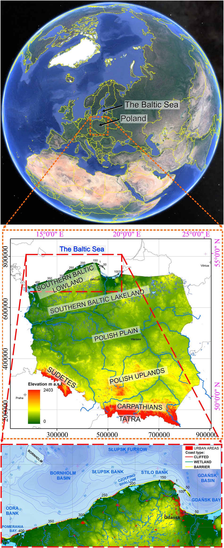
Figure 1. Location of the study based on Google Earth Pro: Landsat/Copernicus, U.S. Department of State Geographer, © Google. Data from SIO, NOAA, U.S. Navy, NGA, GEBCO. Closeup: modified from CBDG of PGI-NRI, coordinate system ETRS1989 PL-1992 (EPSG 2180). The Baltic Sea contour originates from https://tapiquen-sig.jimdofree.com/ accessed on June 5, 2020.
METHODS
Operating principle of the 4F model
The operating principle of the 4F model employs polynomial regression within the functional programming (FP) framework of baselines (frontiers: extents of glacial phases, coastlines) with the aim of assessing deglaciation and coastal development dynamics. Adequate representation accuracy by the model is ensured by high coefficient of determination (R 2) values between the input data and the observed outcomes, as well as through GIS validation of the Desmos model within the 4F model framework.
Common erosion rate calculation methods include plotting lines perpendicular to shorelines via endpoint rate, linear regression, or applying a minimum description length criterion (Crowell et al., Reference Crowell, Douglas and Leatherman1997). However, unlike coastal monitoring and behaviour predicting across the shore via a limited number of transects (i.e., Saye et al., Reference Saye, van der Wal, Pye and Blott2005; Brooks and Spencer, Reference Brooks and Spencer2010; Bagdanavičiūtė et al., Reference Bagdanavičiūtė, Kelpšaite and Daunys2012; Castedo et al., Reference Castedo, de la Vega-Panizo, Fernández-Hernández and Paredes2015), the approach introduced in this paper allows for real-time adjustable alongshore explorations. Here, alongshore quasi-continuous explorations are based on an infinite number of virtual averaged n-profiles (Frydel et al., Reference Frydel, Mil, Szarafin, Koszka-Maroń and Przyłucka2017). Calculations are executed by qualitative graphical modelling of polynomial functions (justified by the increase in the model precision) followed by integral calculus on the fly. Thus, based on a nested table, a nested dynamics model is derived that responds in real time to input changes applied while modelling and retains the ability to test and simulate input ranges at declared intervals.
Programming is achieved within the Desmos environment. Desmos is a freely available, online (cloud-based) advanced graphing calculator written in a JavaScript programming language, which allows plotting of formulae (i.e., equations and inequalities) based on input data, including interactive variables (or constants). Each polynomial function applied reproduces the course of the coastline or range of glacial phase from a table of x,y coordinates acquired from a GIS, such as ArcMap (ESRI), which is a suite commonly used to analyse geospatial data. Geometric analyses of geospatial data are fulfilled within a spatial matrix using high-degree polynomials, whose modelling can be supported by manual adjustments following base maps incorporated into a programme. Afterwards, the results of the integral calculus of polynomial functions assigned within the matrix (representing the ETRS 1989 PL-1992 coordinate system, EPSG 2180; see https://epsg.io/2180) are required to calculate the dynamics coefficients, which are inserted into a secondary table (nested table) where transformation of spatial relationships into coastal development dynamics as a function of time occurs based on equations by Frydel et al. (Reference Frydel, Mil, Szarafin, Koszka-Maroń and Przyłucka2017) modified in this paper, in order to create a nested model, responsive to input modifications and allowing for simulation process.
The 4F model's algorithms consist of adjustable and expandable formulae that provide real-time, precise and explicit outputs, allowing both retrospective analyses of glacial and coastal development dynamics and modelling for coastal management purposes in the future. The described approach is the key input into the 4F morphodynamic model, which utilises developmental factors with a minus sign (−) to indicate ice-sheet retreat, marine regression, or coastal accretion/accumulation and a plus sign (+) for ice-sheet advance, marine transgression, or coastal erosion. Therefore, the 4F model transforms clearly defined equations describing the signatures of state of space in time into a dynamic model nested as a function of time. Finally, the 4F model utilises functions that, due to their mathematical nature, facilitate application in GIS, other computational knowledge engines (WolframAlfa), programming languages (Haskell, Python, R, Wolfram), and the MATLAB environment. Importantly, Desmos allows content sharing (of graphs, maps, programmes, etc.) using so-called permalinks—permanent links that remain unchanged over time, used within this paper to display results developed within the 4F model framework.
FP is a low-level paradigm wherein programs are constructed by applying and composing functions based on a so-called declarative programming paradigm, which in the case of the 4F model returns dynamics of a geologic process resulting from geometric relations between consecutive developmental phases, acknowledged by particular polynomials describing the state of the coastline in time. FP has its roots in lambda calculus—a formal system of computation based on functions only. This, in turn, is a language related to the basics of mathematics used as independent abstract creations or, as in this case, to describe the reality, that is, the state of the boundary lines—coastlines or the extents of deglaciation phases. The FP formulae remain intuitively assembled, developed, and debugged while the programme is being executed, creating results dependent on the previously defined functions and their components. FP also utilises reusable modules to reduce programming time for further tasks (Hughes, Reference Hughes and Turner1990). Despite the presence of FP as a topic within conferences and workshops across the world, this is the first time FP has been applied for the purpose of frontier developmental dynamics studies (of glacial phases and coastlines) within a freely accessible, online matrix.
Simplified scheme of frontier (i.e., glacial extents, coastlines) development—formula derivation applied within the 4F model foundation
Estimation of the average rate of coastal behaviour for a particular shore segment using known positions of the shoreline between initial and final time frames is a known method. However, application of this approach to construct a mathematical model based on polynomial interpolation of the inputs (nodal points) followed by the integral calculus while retaining the ability to adjust the variables allows for a fully responsive, nested model that depicts the outputs in the form of dynamics of change in the time function. Therefore, the concept of a uniform approach to developmental dynamics (${\rm C}_{t_1\to t_2}$ ) between t 1 and t 2 time intervals requires that individual states of the coastline are defined over time by means of successive functions. Consider the geospatial state of the coastline at the initial time (t 1) is determined by the function y 1 = f(x), the coastline at present (t 2) as y 2 = g(x), and the projected coastline at (t m) as y 3 = h(x). Given functions (y 1, y 2, y 3) have the form of the nth power polynomial, whose parameters’ values range from a 0, a 1… to a n. An example scheme of coastline developmental dynamics, for simplification purposes expressed as quartic polynomials, is shown in Figure 2. This uniform approach towards morphodynamics is executed in a user-friendly, open-source, adjustable programme run in a coherent environment, capable of multiscale plotting of characteristic morphometric features and their analysis and accurate calculations, which delivers an instant description of shift dynamics of coastline evolution during the programmed time span. Whenever possible, data inputs are defined as variables (instead of constants), which are preferred due to their flexibility of application in the simulation process. The calculation results within the 4F model framework have high accuracy of feature reproduction demonstrated by high coefficient of determination (R 2) values. The following formulae were applied to ensure that the objectives are met, and based on Frydel et al. (Reference Frydel, Mil, Szarafin, Koszka-Maroń and Przyłucka2017), the averaged shift dynamics factor was defined as:
where
${\rm C}_{t_1\to t_2}$ is the averaged shift dynamics (ice-sheet retreat or advance/marine transgression or regression/coastal erosion or accretion/accumulation; expressed in m/yr,
A t1t2 is the area between t1 and t2 (projected on the x,y plane; expressed in m2),
t 1 is the time moment for the first data series,
t 2 is the time moment for the second data series,
t is the number of years (interval) between t 1 and t 2; expressed in years, yr, and
B ∈ 〈x u, x l〉 is the baseline length (integral limit; expressed in meters, m).
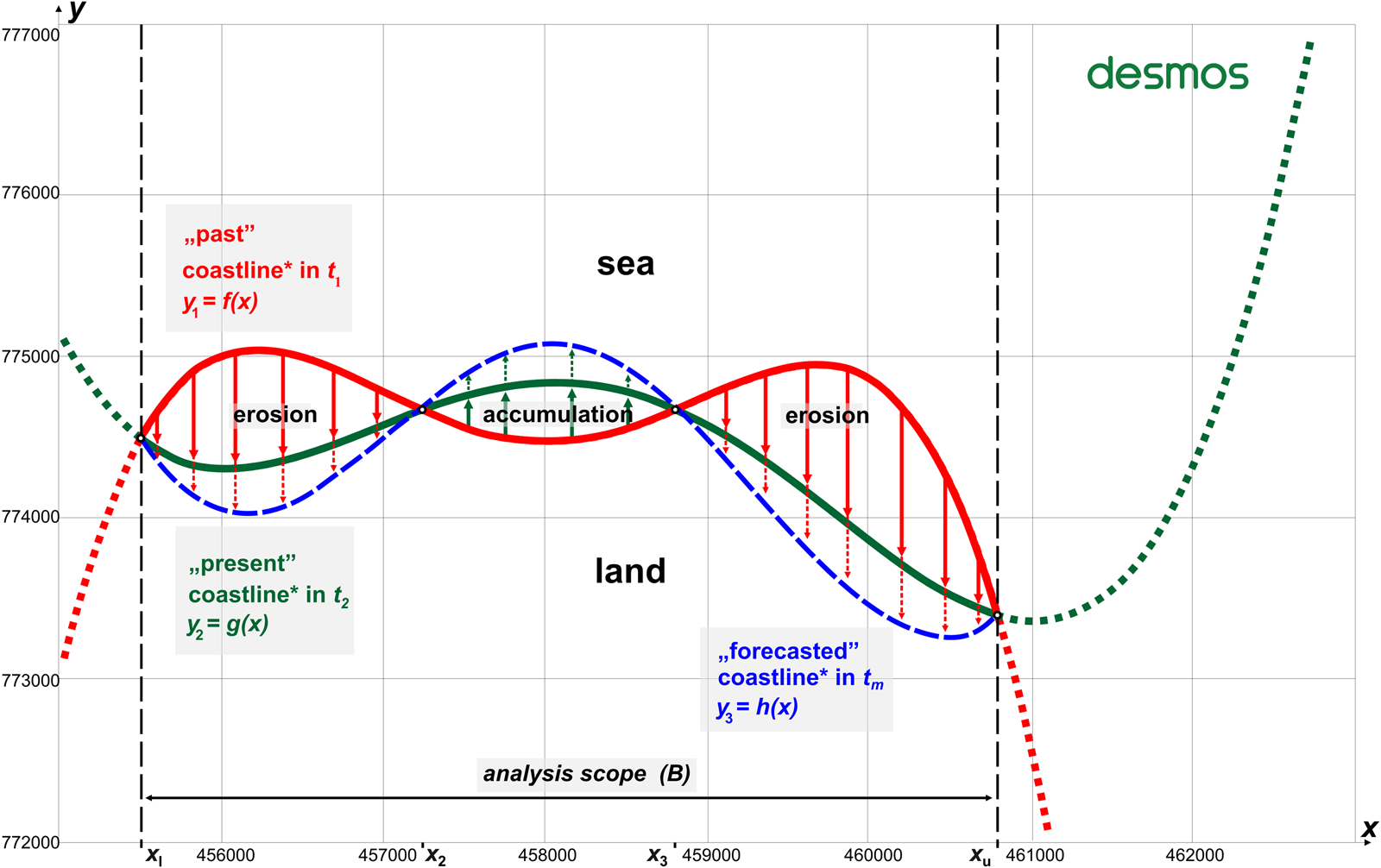
Figure 2. Schematic basic model of coastline development expressed as quartic polynomials (4th order) in the past (red): y 1 = f(x); current state (green): y 2 = g(x); and forecast coastline location (blue): y 3 = h(x). Recognised developmental tendencies are indicated with arrows: erosion in red; accumulation/accretion in green; dashed arrows of respective colours define forecast extents for given transects. By definition, the geospatial location of this hypothetic coastlines (and the assignment of coordinates at the x and y axes) are expressed directly by formulae of individual polynomials (y 1,y 2, y 3), in this case, within the Cartesian coordinate system PL-1992 (EPSG 2180), while points x l, x 2, x 3, and x u define the limits of shift dynamics integration intervals R 2 ∈ 〈0.9912, 0.9996〉.Footnote 1
By adaptation of Eq. 1, the shift dynamics factor (developmental dynamics factor) was encoded in Unicode (U+03F9) by lunate sigma (C) for the given time range between t m−1 and t m $( {{\rm C}_{t_{m-1}\to t_m}} )$ . The shift dynamics, conceived as an accumulated rate of coastline changes $( {{\rm C}_{t_{m-1}\to t_m}} )$
 averaged along the segment between the integral limits, the lower (x l) and upper one (x u), which stand for the longshore analyses scope (B), is calculated by the formula:
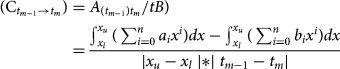
where n ∈ N, m ∈ N; n is the polynomial degree; and m is the time interval number. An area indicated by Frydel et al. (Reference Frydel, Mil, Szarafin, Koszka-Maroń and Przyłucka2017) as A t1t2 is then calculated as a difference between the integral of f(x) and the integral of g(x), as shown in Figure 2 (for which n = 4). Shift dynamics with positive (+) values define the dynamics of ice-sheet advance inland (glaciation), the Baltic Sea transgression, coastline retreat or coastal erosion $( {\rm C}_{t_{m-1}\to t_m} > 0)$ , resulting from Eq. 2. Identified regions are then displayed and highlighted instantly (using a desired colour) by the application of a double inequality in the form of:
Shift dynamics with negative (−) values define the dynamics of ice-sheet retreat (deglaciation/decay), the Baltic Sea regression, coastline advance, coastal accretion/accumulation $( {\rm C}_{t_{m-1}\to t_m} < 0)$ , resulting from Eq. 2. Identified regions are displayed and highlighted immediately by the application of a double inequality, in the form of:
Consequently, as shown in Figure 2, the 4F model foundation programmed in the manner described provides the ${\rm C}_{t_1\to t_2}$ value, which allows modelling and calculation of the forecast (extrapolated) range and the coastal development dynamics (erosion/accumulation) ($F_{t_2\to t_m}$
 ) in real time for the desired number of years (time span, p) specified as:

*The result of Eq. 5 contains an extrapolated value of the previously recognised trend. Yet projections of future shift dynamics tendencies based on actual data were determined in accordance with the extended methodology presented in the next section.
Using Figure 2 and Eqs. 1–5, the calculated factors reveal the quantitative change in the past and the forecast values (Supplementary Table 1). Along with the polynomial parameters (specified in Supplementary Table 2), which stand for the qualitative position of the coastline (Fig. 2), they permit dynamic forecasting of the extents of the erosion/accumulation and display regions subject to positive (+, erosion) and negative (–, accretion) shifts. Therefore, Supplementary Table 2 shows a solution for qualitative and quantitative modelling based on polynomial regression within a spatial matrix, which defines successive coastline locations (“past,” “present,” and “forecasted”) in Figure 2. The mechanism described here retrieves numerical values of dynamics (${\rm C}_{t_1\to t_2}$ ) obtained during the quantitative analysis and subsequently designates negative shift tendency (−) for ice-sheet retreat (deglaciation)/marine regression/coastal accumulation; or positive tendency (+) for glacial advance/marine transgression/coastal erosion. Consequently, the main purpose of the basic model is to determine and simulate the dynamics of geologic processes via regression of polynomial functions with their specific parameters followed by the integral calculus. Its schematic representation of the model's operation is shown in Figure 2. The model uses functions, mainly high-order polynomials, to reflect the state of a process, here the extent of a coastline at a particular time (t). This is called modelling via polynomial regression. The model in its basic form utilises polynomials of the fourth degree, so each polynomial function contains five parameters, as specified in Supplementary Table 2. For the purpose of presenting the operation mechanism of the method, values t 1= 1800, t 2= 2000, p = 200 were adopted. It should be emphasised that the location of the functions f(x), g(x), h(x) in the matrix (Fig. 2) were selected arbitrarily. Furthermore, the intersection point of individual functions with the OY and OX axes is irrelevant, because the integration result is the same, regardless of the position of the function in the matrix space, as illustrated in the concept and the operating principle of the 4F model foundation (Fig. 2).
The 4F model baseline inputs, materials, and forecasting mechanism
The model makes it possible to explore developmental tendencies and predict the extent and nature of changes in the future based on the adopted SLR scenarios, analysis of coastline extent limits, and glacial-phase ranges in the past (the course of which, projected onto the x,y plane, exhibits polynomial-like characteristics). Palaeodynamics was inspected using the example of developmental stages of the ice sheet in Poland (and partially neighbouring areas) in the years 24–15 ka BP (MIS 2) followed by the SBS development since the BIL in the years 10.5–10.3 ka BP (MIS 1) until the present time. Long-term future projections during the Anthropocene acknowledge gmsl-rise scenarios. A primary, fully operational model that is adaptable and expandable was constructed in the Desmos environment. Because development of the Baltic coastline in the past was related to the retreat of the Scandinavian ice sheet (Uścinowicz, Reference Uścinowicz, Mojski and Dadlez1995, Reference Uścinowicz1999, Reference Uścinowicz2004, Reference Uścinowicz2006, Reference Uścinowicz, Chiocci and Chivas2014; Marks, Reference Marks2002; Marks et al., Reference Marks, Dzierżek, Janiszewski, Kaczorowski, Lindner, Majecka and Makos2016; Harff et al., Reference Harff, Flemming, Groh, Hünicke, Lericolais, Meschede, Rosentau, Flemming, Harff, Moura, Burgess and Bailey2017; Rosentau et al., Reference Rosentau, Bennike, Uścinowicz, Miotk-Szpiganowicz, Flemming, Harff, Moura, Burgess and Bailey2017; Hall and van Boeckel, Reference Hall and van Boeckel2020), it is justified to use markers such as a range of individual phases of glaciation and consecutive shoreline frontiers for the purpose of modelling. Owing to the development of the methodology presented in the preceding sections, the 4F model was applied to determine the deglaciation palaeodynamics during the late Vistulian period (Weichselian/Würm glaciation), which included the limits of glacial phases during MIS 2, from the Leszno Phase (L, 24 ka BP) (Marks et al., Reference Marks, Dzierżek, Janiszewski, Kaczorowski, Lindner, Majecka and Makos2016), through the Poznań Phase (Poz, 20–19 ka BP), the Pomeranian Phase (Pom, 17–16 ka BP) (Marks et al., Reference Marks, Dzierżek, Janiszewski, Kaczorowski, Lindner, Majecka and Makos2016), the Gardno Phase (G, 16.8–16.6 ka BP), the Słupsk Bank Phase (SB, 16.2–15.8 ka BP) up to Southern Middle Bank Phase (SMB, 15.4–15.0 ka BP) (Uścinowicz, Reference Uścinowicz, Mojski and Dadlez1995, Reference Uścinowicz1999), followed by the Baltic basin development in the Holocene (Uścinowicz, Reference Uścinowicz, Mojski and Dadlez1995, Reference Uścinowicz1999, Reference Uścinowicz2006).
The diagram of the 4F model as well as input and output data scopes illustrating the principle of the operating mechanism of the model are shown in Supplementary Figure 1. Morphodynamic analyses were executed in a review time scale of 24 ka of the Quaternary and a general spatial scale of 1:2,000,000 relating to the SBS, the territory of Poland, and, partially, the adjacent countries. Modelling includes the deglaciation dynamics in the Pleistocene, the development of the SBS in the Holocene, and forecasts of the erosion pace and extent in the Anthropocene (until 7170–25,500 CE) in light of a projected gmsl rise due to ice melting caused by climate change, including temperature increase due to increased greenhouse gas emissions (especially CO2).
The input data for the 4F model comprised maps that represent the results of analyses performed with the use of geologic, geomorphological, and oceanographic research (coupled with radiocarbon dating). Specifically, the 4F model inputs such as time (t 1 to t 16) and baseline geospatial locations were derived from Marks et al. (Reference Marks, Dzierżek, Janiszewski, Kaczorowski, Lindner, Majecka and Makos2016) and Uścinowicz (Reference Uścinowicz, Mojski and Dadlez1995, Reference Uścinowicz1999). They were geocoded using the GIS ArcMap suite in accordance with standard procedures, which were applied in order to view, edit, register, and analyse geospatial data. These actions allowed creating and exporting new maps for further use in the Desmos environment. The root-mean-square (RMS) error of registration (<500 m) was satisfactory for the scale (1:2,000,000), while the coefficient of determination of digitised baselines (ice-sheet ranges, coastal locations) equalled R 2 ∈ 〈0.93, 0.98〉; therefore, the results adequately reflect the geologic evidence for glacial retreat and shoreline migration. High polynomial regression coefficient values ensure the observed outcomes are replicated effectively by the model. Nevertheless, due to the small spatial scale of the study and Desmos limitations, the individual functions were modelled on the basis of a maximum number of 50 vertices distributed along each frontier baseline (glacial extent or coastline) whose position was subject to adjustment to allow better course reproduction. Secondary base maps of sea and land included DEMs along with other vector graphics (e.g., hydrological and urban), while classification of the Polish coasts of the SBS (cliffs, barriers, wetlands) at a scale 1:200,000 based on the typology by Uścinowicz et al. (Reference Uścinowicz, Zachowicz, Graniczny and Dobracki2004) were obtained from the Central Geological Database of the Polish Geological Institute–National Research Institute (CBDG of PGI-NRI). Geostatistical data (at 1 km resolution) concerning demographic distribution of the population in Poland are from the 2011, census while the relief DEMs (at 100 m spatial resolution) are from a governmental source (Head Office of Geodesy and Cartography, GUGIK).
The nested graph of developmental dynamics of the SBS coasts in the Anthropocene was designated for three projections of the future gmsl equalling +2 m, +5 m, and +65 m asl, the last of which describes Earth in a virtually ice sheet–free scenario. To maintain adaptability, variable time intervals for each scenario were assigned in the 4F model in line with the projected SLR (Oppenheimer et al., Reference Oppenheimer, Glavovic, Hinkel, van de Wal, Magnan, Abd-Elgawad, Cai, Pörtner, Roberts, Masson-Delmotte, Zhai, Tignor, Poloczanska and Mintenbeck2019; Golledge, Reference Golledge2020). The analysis of the northern Polish coasts at risk of flooding related to SLR was developed based on the quantitative criteria of Ridley et al. (Reference Ridley, Gregory, Huybrechts and Lowe2010) and Grant et al. (Reference Grant, Naish, Dunbar, Stocchi, Kominz, Kamp and Tapia2019), followed by separate application of RCP8.5 and RCP2.6 (representative concentration pathway) scenarios by Oppenheimer et al. (Reference Oppenheimer, Glavovic, Hinkel, van de Wal, Magnan, Abd-Elgawad, Cai, Pörtner, Roberts, Masson-Delmotte, Zhai, Tignor, Poloczanska and Mintenbeck2019) and Golledge (Reference Golledge2020). Then, each DEM created in GIS was imported and adapted within the Desmos matrix. The 4F model maintained a uniform time scale between past, present, and future to assure matrix consistency between inputs and in line with the beginning of the Anthropocene in 1950 as postulated by Waters et al. (Reference Waters, Zalasiewicz, Summerhayes, Barnosky, Poirier, Gałuszka and Cearreta2016). For this reason, x = 0 on the OX axis within the nested matrix represents the year 1950 adopted as “present” time. Values with a negative sign (−), to the left of the OX axis indicate projected coastal dynamics in the future, while the values on the right (+) correspond to the past.
The range of remote sensing data available for larger-scale analyses includes satellite data, aerial photographs, and detailed, repetitive results of airborne LIDAR conducted on behalf of maritime authorities since 2008, terrestrial LIDAR data acquired by PGI-NRI since 2010, and hydroacoustic data from the nearshore zone. Availability of individual data sets varies from region to region due to differences in local maritime policies.
The 4F model principles
The main purpose of the 4F model is to determine and simulate the dynamics of geologic processes; a schematic representation of the basic model's operation is shown in Figure 2. Those processes may represent two different directions of developmental vectors: negative (−) and positive (+) ones. Negative (−) values were assigned to ice-sheet retreat (deglaciation), marine regression, and coastal accumulation; whereas processes with a positive (+) value include ice-sheet advance, marine transgression, and coastal erosion. The 4F model framework is available online and consists of 273 modules containing tables, functions, equations, inequalities, graphs, base maps, and notes. A description of palaeogeography and palaeodynamics over a period of 24 ka is created within the digital environment of Desmos graphing calculator (https://www.desmos.com/calculator/29lkndchee, accessed on 28/07/2021) based on the premises of the FP of the spatial matrix with the use of polynomial regression and integral calculus. The model uses functions, mainly high-order polynomials, to reflect the state of a process, for instance, the extent of an ice sheet or the location of a coastline at a particular time, which is called modelling via polynomial regression. State representation is achieved within an orthogonal (square) or polar matrix. The model in its current form utilises 15th to 19th degree polynomials in a square matrix (EPSG 2180). Further attempts to plot the functions even more accurately using polynomials, of degree 20 and above, despite initial increase of R 2 from 0.95 (Fig. 4A) to 0.97 (Fig. 3), finally resulted in a collapse of the function (Fig. 3, C–D) (R 2 = −0.95 to R 2 = −59.27). Model consists of 15 main functions that stand for subsequent states of evolution of the area during deglaciation (6 functions), followed by Baltic Sea evolution (6 functions), and projections of Baltic Sea extent in the future (3 functions) at a specific time (t). The next step involves executing the integral calculus on the basis of the determined functions and then calculating the numeric result of the two definite integrals for successive developmental stages within the specified spatial range (B, ∈ 〈x u, x l〉). Particular formulae represent the geometric relations between the ranges of individual phases of Scandinavian ice-sheet retreat (deglaciation) during the late Pleistocene (MIS 2, late Vistulian) along with subsequent positions of the Baltic coastline in central Europe (especially Poland) during the Holocene (MIS 1). The result of the calculation is substituted into Eq. 2. With the results for all subsequent stages of development obtained in the same way, a secondary table is constructed containing the individual developmental dynamics coefficients (${\rm C}_{t_{m-1}\to t_m}$ ) and timestamps from t 1 to t 16. As a result of displaying the secondary table within the nested matrix, a graph of changes in the dynamics of the analysed processes through time was obtained (with time t within the horizontal axis scaled by 10−1). Consequently, the postulated approach utilised palaeogeography to form palaeodynamics (dynamics as a function of time). Finally, the common glacial dynamics and coastal dynamics developmental model and its algorithms introduced here—the 4F model—consist of adjustable and expandable formulae and provide a real-time, precise, and explicit output for dynamics mapping and simulation of past and future geologic processes. An additional technical overview of the 4F model can be found in Supplementary Text 1.
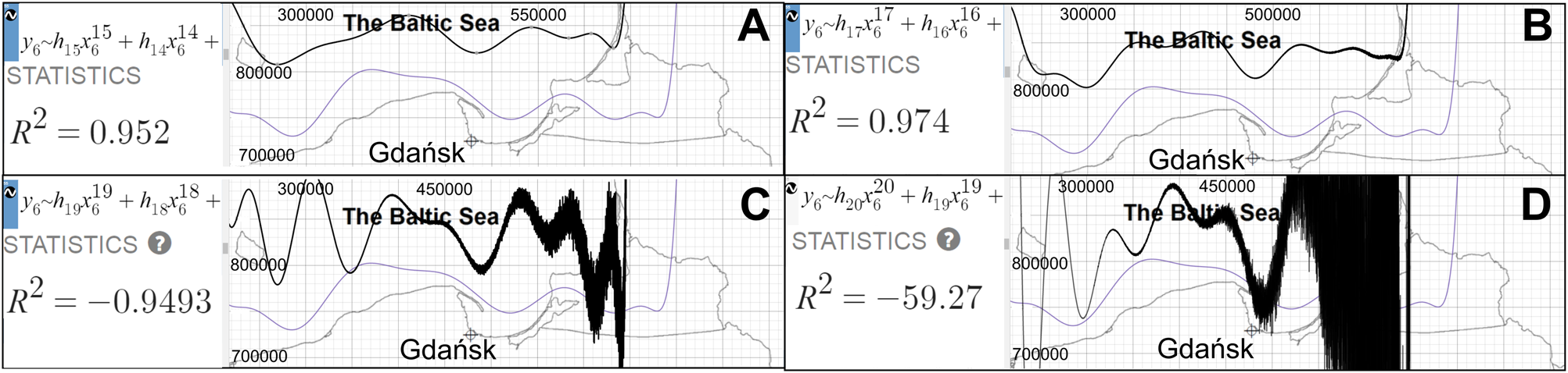
Figure 3. Exploration of function limitations in the Desmos environment visualised via systematic deterioration of f 6(x) (Southern Middle Bank Phase [SMB], black) as polynomial order increases: (A) 15th order, R 2 = 0.952; (B) 17th order, R 2 = 0.974; (C) 19th order, R 2 = −0.9493; (D) 20th order, R 2 = −59.27. The figure shows the steps involved while modelling with polynomials of increasing degree. As the degree of the polynomial increases, the quality of the representation decreases. This is reflected in the value of the correlation coefficient.
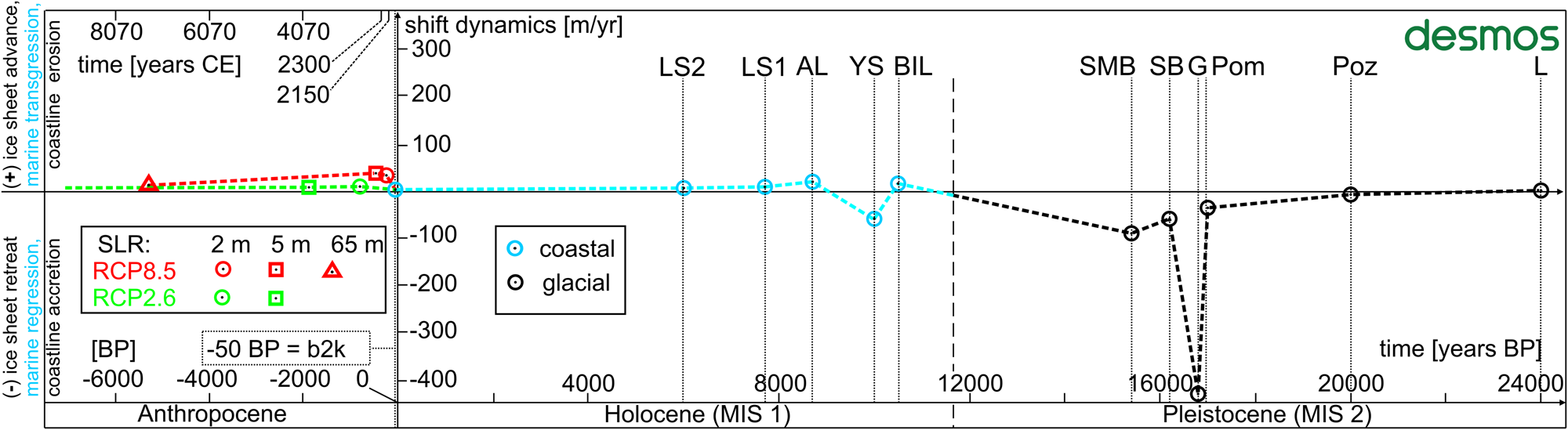
Figure 4. Nested model of shift dynamics in the time function (dashed line) of the Scandinavian ice-sheet recession in the late Pleistocene (Marine Oxygen Isotope Stage 2 [MIS 2]) based on Marks (Reference Marks2002) and Marks et al. (Reference Marks, Dzierżek, Janiszewski, Kaczorowski, Lindner, Majecka and Makos2016) (black); the development of the SBS in the Holocene (MIS 1) (blue) (Uścinowicz, Reference Uścinowicz, Mojski and Dadlez1995, Reference Uścinowicz1999); and forecasts of the pace and extent of erosion in the Anthropocene, in the light of projected gmsl-rise RCP8.5 and RCP2.6 scenarios: red, Oppenheimer et al. (Reference Oppenheimer, Glavovic, Hinkel, van de Wal, Magnan, Abd-Elgawad, Cai, Pörtner, Roberts, Masson-Delmotte, Zhai, Tignor, Poloczanska and Mintenbeck2019), and green, Golledge (Reference Golledge2020), modified from the 4F model nested matrix. The Desmos icon contains a hyperlink to the 4F model, last accessed on February 4, 2021.
Significantly, the morphodynamics is a parameter derived from the shore's resistance to destruction; it is inversely proportional to the strength of resistance, with clear link between higher rate of erosion and a weaker shore involved. Assembly of this tool allows graphing of developmental dynamics of ice-sheet advance/retreat, marine transgression/regression, and coastal erosion/accumulation processes, within a coherent matrix that guarantees the ability of further modifications to be included in the future.
RESULTS OF THE 4F MODEL IMPLEMENTATION
The 4F model, implemented within the Desmos environment, which represents coherent space–time relations, made it possible to pinpoint deglaciation frontier positions of the Scandinavian ice sheet during the late Vistulian glaciation and the subsequent coastlines during the development of the Baltic Sea in the Holocene. Positions of the frontiers, glacial and coastal, were assigned through a high-level polynomial regression within consistent time frame of 24 ka during MIS 1 and MIS 2. In subsequent calculations, integral calculus applied on successive polynomials for the purpose of shift dynamics factors calculation, made it possible to create a consistent time–dynamics model (Fig. 4). The nested model revealed the dynamics of these processes (glacial dynamics, coastal dynamics) over time, facilitated correlation of the late Pleistocene ice-sheet deglaciation characteristics with climatic changes and correlation of further relative sea-level changes of the SBS during marine transgression and regression phases. Eventually, the nested part of the 4F model also provided primary insights into the future dynamics of the SBS development in the Anthropocene, reflecting gmsl-rise scenarios applied from DEMs.
Glacial dynamics in Poland during the late Pleistocene (MIS 2)
The dynamics parameter compatibility of the 4F model in the Desmos environment with the GIS environment ranges from 95.9% to 99.9%. As shown in Figure 5, the recession dynamics of the Scandinavian ice sheet in the late Pleistocene in Poland were determined for an interval of 8.6 ka, beginning with the L Phase (24 ka BP) up to the SMB Phase (15.4 ka BP). Initially, until the Poz Phase (20 ka BP), the deglaciation dynamics was modest at −8.5/ma and gradually accelerated to −37.2/ma in the Pom Phase (17 ka BP). A significant, peak increase in the recession rate of −427.3 m/yr (max. −861.4 m/yr) occurred during Heinrich event H1, particularly up to the G Phase (16.8 ka BP). Thereafter, until the SB Phase (16.2 ka BP), the dynamics of the ice-sheet retreat was still high at −60.5 m/yr and accelerated again to −90.7 m/yr by the SMB Phase (15.4 ka BP). Significantly, a diagram of deglaciation dynamics in the time function originating from the nested matrix of the 4F model allowed the ice-sheet recession dynamics to be linked to the palaeoclimatic reconstructions in the Tatra Mountains. Consequently, the modelling results confirm that the most dynamic ice-sheet retreat occurred during the late-glacial interstadials: LG1 and LG2 (within the H1 event).
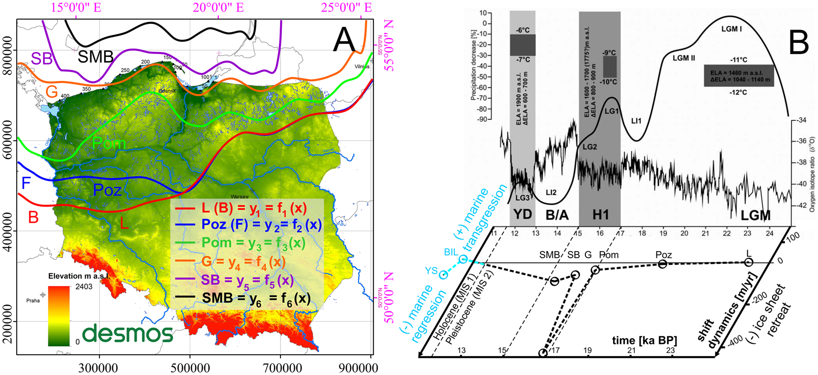
Figure 5. (A) Palaeogeographic reconstruction of the phase ranges: L, Leszno Phase (B, Brandenburg Phase); Poz, Poznań Phase (F, Frankfurt Phase); Pom, Pomeranian Phase; G, Gardno Phase; SB, Southern Baltic Phase; SMB, Southern Middle Bank Phase; modified from the 4F model. The Desmos icon contains a hyperlink to the 4F model, last accessed on February 4, 2021. (B) Summary of palaeoclimatic reconstructions in the Tatra Mountains originates from Marks (Reference Marks2002) and Marks et al. (Reference Marks, Dzierżek, Janiszewski, Kaczorowski, Lindner, Majecka and Makos2016) and is supplemented with the diagram of deglaciation dynamics in the time function from the current study (Fig. 4); dashed line indicates the pace of ice-sheet retreat in m/yr; solid black line shows changes of relative glacial extent during subsequent advances in the study area. Glacial phases: L, Leszno; Poz, Poznań; Pom, Pomeranian; G, Gardno; SB, southern Baltic; SMB, Southern Middle Bank. SBS development phases (Uścinowicz, Reference Uścinowicz, Mojski and Dadlez1995, Reference Uścinowicz1999): BIL, Baltic Ice Lake; YS, Yoldia Sea; LGM, last glacial maximum; LG1–3, late-glacial stadials 1–3; LI1–2, late-glacial interstadials 1 and 2; B/A, Bolling/Allerod interstadial; YD, Younger Dryas; H1, Heinrich event 1; ELA, equilibrium line altitude of glacier (modified from Marks et al., Reference Marks, Dzierżek, Janiszewski, Kaczorowski, Lindner, Majecka and Makos2016), coordinate system ETRS 1989 PL-1992 (EPSG 2180).
SBS coastal dynamics in the Holocene (MIS 1)
The dynamics compatibility of the 4F model in the Desmos environment with the GIS environment ranges from 92.6% to 99.1%. As shown in Figure 6, through application of Eq. 2 upon a spatial matrix, the 4F model addressed palaeodynamic aspects of SBS development within the nested time–dynamics matrix consistent with previous analyses. In this respect, it has been recognised that after the SMB (15.4 ka BP), the development of the SBS coastline frontiers towards the BIL (10.5 ka BP), transgression proceeded at a pace of 16.5 m/yr. By the end of the BIL, the isostatic terrain uplift resulted in a rapid water-level decrease followed by the Baltic coastline recession at a rate of −56.8 m/yr (max. −128.7 m/yr) to the Yoldia Sea (YS; 10 ka BP), when, due to eustatic SLR, a connection with the Atlantic Ocean was formed, allowing for a transgression towards the Ancylus Lake (AL; 8.7 ka BP) at a pace of 21.4 m/yr. Since then, the transgression dynamics gradually decreased. Following the AL, the dynamics of further transgression towards the Littorina Sea 1 (LS1; 7.7 ka BP) and the Littorina Sea 2 (LS2; 6 ka BP) and, finally, the developmental dynamics of the current coastline (approx. 2000 CE, −50 yr BP) diminished by 9.3 m/yr, 2.2 m/yr and 0.4 m/yr, respectively, all of which correlate well with the SLR curve for the SBS (Fig. 6).
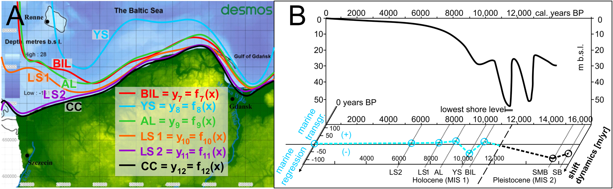
Figure 6. Palaeogeography (A) and palaeodynamics of the Southern Baltic Sea (SBS) development in the Holocene in the light of the relative sea-level rise (SLR) curve (Uścinowicz, Reference Uścinowicz, Mojski and Dadlez1995, Reference Uścinowicz1999, Reference Uścinowicz2004, Reference Uścinowicz, Chiocci and Chivas2014), modified from the 4F model, the Desmos icon contains a hyperlink to the 4F model, last accessed on February 4, 2021. (B) Relative SLR curve for the SBS (modified from Uścinowicz, Reference Uścinowicz2004, Reference Uścinowicz, Chiocci and Chivas2014; and supplemented with the Baltic developmental dynamics from the current study. See Fig. 5 for definitions of abbreviations.
Preliminary insights into projected SBS transgression dynamics in the Anthropocene
The dynamics compatibility of the 4F model in the Desmos environment with the GIS environment ranges from 46.6% to 82.7%. As recognizing past changes is the key to understanding future changes, the coherent matrix of the 4F model permitted the casting of long-term projections of future transgression extents and dynamics in the Anthropocene at a general spatial scale and time scale (Fig. 7), consistent with the results described within previous sections. Extrapolation under assumption of the linear rate of SLR was performed for projections in the <RCP8.5, RCP2.6> range, which approximates both the nature and the spectrum of potential scenarios. Consequently, application of gmsl-rise scenarios, analysed on the basis of DEM data, suggests that a 2 m increase in the world's ocean by 2190–2720 CE will be associated with transgression dynamics in the range of 23.9–38.2 m/yr. As a result, as many as 684,000 people, including 3400 km2 of terrain, will be exposed to flooding (Fig. 7A). The model also defines the most vulnerable areas of the Polish coastal zone in the future. The largest and the most threatened areas include the Żuławy Wiślane, a vast area of the alluvial delta of the Vistula River, which includes depression areas that are still inhabitable due to a widespread drainage system. Inflows of salty Baltic waters may reach as far as 40 km inland. The Hel Peninsula is likely to undergo periodic storm breaks in its western part, with the simultaneous accumulation of eroded material in the vicinity of the southeastern part of the promontory.
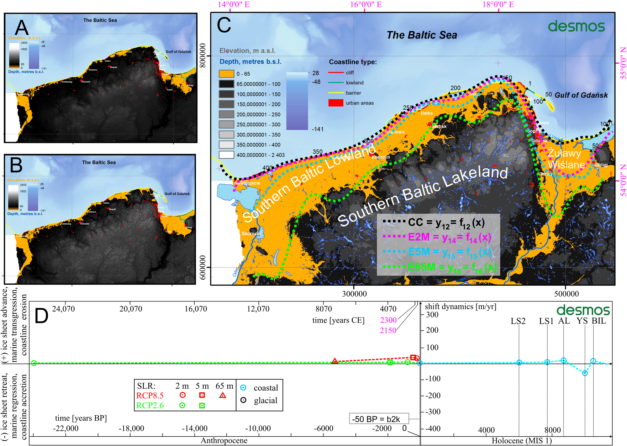
Figure 7. Projection of the Southern Baltic Sea (SBS) extent in the Anthropocene based on gmsl-rise RCP8.5 and RCP2.6 scenarios: (A) sea-level rise (SLR) by 2 m by 2190–2720 CE; (B) SLR by 5 m by 2400–3800 CE; (C) SLR by 65 m (ice sheet–free Earth); consecutive functions marked with dotted lines correspond to each scenario: (A) purple; (B) blue; (C) green; dotted black line represents the current coastline, modified from the 4F model, coordinate system ETRS 1989 PL-1992 (EPSG 2180). The Desmos icon contains a hyperlink to the 4F model, last accessed on February 4, 2021. See Fig. 5 for definitions of abbreviations.
Thereafter, a 5-m-high increase (Fig. 7B) of gmsl (by 2400–3800 CE) will be associated with an increase of averaged transgression dynamics ranging from 26.8–46.4 m/yr. Floodplains are likely to encompass an area of nearly 50 km inland in the Vistula delta region. At this time, sandy barrier coasts will be subject to extensive erosion, while coastal lakes will suffer from Baltic ingressions, and the overall number of coastal zone inhabitants affected by negative land transformations will reach 841,400, with 4480 km2 of terrain also being affected.
The last projection (Fig. 7C) corresponds to a 65-m-high gmsl rise when Earth becomes essentially glacier-free due to global warming. Catastrophic consequences will cover the area of the young glacial relief subprovinces associated with Pleistocene glaciations (the Southern Baltic Lowland) and parts of the Southern Baltic Lakeland, especially in the Vistula valley area. As a result, more than 3 million people (3,144,000) will have to face the consequences of landscape transformation, while the inhabitable zone is likely to shrink by 18,280 km2. The SBS inflow and ingression vectors will extend inland as far as 108 km, 26–33 km, and 260 km, respectively, in the eastern, central, and western parts of the Polish coastal zone. Despite great uncertainty behind this scenario, it is possible it will be fulfilled within 7170–25,500 CE, based on linear extrapolation of growth rates described in two previous projections.
DISCUSSION
In Poland, coastal preservation policies in the twenty-first century are based on coastal morphodynamics, developmental trends, and protective methods and strategies (Zawadzka-Kahlau, Reference Zawadzka-Kahlau1999, Reference Zawadzka-Kahlau2012; Łęczyński, Reference Łęczyński2009; Dudzińska-Nowak, Reference Dudzińska-Nowak2015). They are considered and implemented by maritime authorities. The future of shore protection by 2050 includes technical activities related to the protection of material and natural assets within the endangered areas of the coastal hinterland, based on the diagnosis of endangered areas obtained by monitoring changes in the location of the coastline. Consequently, the following technical coastal protection strategies should be considered in the long-term: withdrawal from the affected area without further actions; partial protection of the most endangered stretches of the coastline; control of erosion along the entire length of the coastline; and expansion. Under current legislation, direct protection of the seashore is the responsibility of the maritime authorities in Gdynia, and Szczecin. The results of the 4F model described in this paper defined the areas at risk of erosion or flooding and display their properties and the transgression dynamics.
Morphodynamic models for coastal application
The use of numerical models to simulate shoreline changes has a long history. Among the undoubted advantages of such models is their simplicity and range of applications (Hanson, Reference Hanson1989). In environments subject to intense erosion with a direct impact on tourist-based economies, they enable recognising and forecasting coastal changes (Genz et al., Reference Genz, Fletcher, Frazer and Rooney2007). Morphodynamic models have been compared with analytical morphodynamic theories (Zolezzi et al., Reference Zolezzi, Vanzo, Siviglia and Stecca2013) and developed as a process-based form. They have also been successfully used so far both in soft-rock Quaternary environments of the southern Baltic coast (Zhang et al., Reference Zhang, Harff, Schneider, Meyer and Wu2011, Reference Zhang, Schneider, Kolb, Teichmann, Dudzinska-Nowak and Harff2015) and in rocky coast development (Matsumoto et al., Reference Matsumoto, Dickson and Kench2016). Reconstructions and forecasts of coastal development in the SBS area on a regional scale made by Deng et al. (Reference Deng, Zhang, Harff, Schneider, Dudzinska-Nowak, Terefenko and Giza2014, Reference Deng, Harff, Zhang, Schneider, Dudzinska-Nowak, Giza, Terefenko, Harff, Furmańczyk and von Storch2017) confirm the validity of the use of morphodynamic models for practical application in coastal zone management. In the area of the SBS, the most intense shoreline displacements due to rapid water-level increase at a rate of up to approx. 40–45 mm/yr occurred during consecutive phases of Baltic Sea development between the late glacial and Early Holocene (Uścinowicz, Reference Uścinowicz2004). In turn, detailed geologic surveys of coastal behaviour were included in the 4D Cartographic Project (Kramarska et al. Reference Kramarska, Uścinowicz, Jurys, Jegliński, Przezdziecki, Frydel and Tarnawska2014; Uścinowicz et al., Reference Uścinowicz, Lidzbarski, Pączek, Dąbrowski, Jasiński, Szarafin and Jurys2018) carried out by the Polish Geological Survey (PSG). This project also involved mapping of landslide susceptibility with regard to a geologic structure, longshore sediment transport (Uścinowicz et al., Reference Uścinowicz, Lidzbarski, Pączek, Dąbrowski, Jasiński, Szarafin and Jurys2018), and slope stability issues (Jasiński et al., Reference Jasiński, Pacuła, Dąbrowski, Badura, Uścinowicz, Szarafin, Jurys, Witak, Pędziński and Trzcińska2018) based on a finite element method (Dąbrowski et al., Reference Dąbrowski, Krotkiewski and Schmid2008). The past variability of developmental tendencies of cliffed coasts as well as barrier coasts in Poland was clearly associated with different intensity of hydrometeorologic conditions (Furmańczyk et al., Reference Furmańczyk, Dudzińska-Nowak, Furmanczyk, Paplinska-Swerpel and Brzezowska2012; Dudzińska-Nowak and Wężyk, Reference Dudzińska-Nowak, Wężyk, Green and Cooper2014; Kostrzewski et al., Reference Kostrzewski, Zwoliński, Winowski, Tylkowski and Samołyk2015; Dudzińska-Nowak, Reference Dudzińska-Nowak, Harff, Furmańczyk and von Storch2017).
As shown in this paper, based on hindcasts for the late Vistulian glaciation (Weichselian/Würm glaciation) (after Marks et al., Reference Marks, Dzierżek, Janiszewski, Kaczorowski, Lindner, Majecka and Makos2016) and the Baltic coastal development (after Uścinowicz, Reference Uścinowicz2006) described within the same coherent timeline (Fig. 4), the current approach facilitates the enhancement of further relative sea-level reconstructions (Berglund, Reference Berglund2004; Miettinen, Reference Miettinen2004; Karlsson and Risberg, Reference Karlsson, Risberg, Johansson and Lindgren2005; Linden et al., Reference Linden, Möller, Björck and Sandgren2006; Lampe et al., Reference Lampe, Meyer, Janke, Ziekur, Janke, Endtmann, Harff and Lüth2007) and projections of the Baltic Sea coastal behaviour on a similar basis. Furthermore, after necessary modifications, the 4F model can also be applied in other domains, for example, for modelling the dynamics of the Laurentide Ice Sheet and glaciations in the Alps (Eburonian, Elsterian, Saalian, Weichselian). However, based on the present version of the 4F model, a direct opportunity already exists to extend it for the purpose of determining the dynamics of ice-sheet development in Poland over approx. 1 million years (since the Narew glaciation).
In the end, among the challenges for the future is to link the hydrometeorologic conditions, geologic structure, and the presence of coastal engineering with the variability of the coastal zone dynamics at local (Frydel, J.J., unpublished data) and regional scales. However, certain issues of sustainable management for future generations remain unsolved, including the adoption of strategies that will maintain a balance between security, economic outlook, and an approach that favours the conservation of the natural qualities of the landscape requiring the least human intervention.
4F model assessment: comparison, uncertainties, strengths, weaknesses, and validation
Within the predictive part of the 4F model, similar to the work of Meyer (Reference Meyer2003), scenarios of future shoreline changes were analysed based on three main components: DEM, eustatic sea-level changes, and influence of isostasy. Contrary to Meyer (Reference Meyer2003), in the case of Polish coasts, the trend of crustal changes due to isostasy is near zero (or slightly negative), depending on the exact location (Graniczny et al., Reference Graniczny, Čyžienė, van Leijen, Minkevičius, Mikulėnas, Satkūnas and Przyłucka2015). Therefore, acknowledged impacts were excluded from the model as being negligible. In contrast, the DEM used here (0.1 × 0.1 km) is more accurate than the one used by Meyer (Reference Meyer2003) (1 × 1 km). However, both DEMs are useful only for large-scale purposes (for the area of the whole country), while DEMs with higher horizontal resolution (and higher vertical accuracy) are required for local studies. For the area of Poland, a DEM from the nationwide Informatyczny System Osłony Kraju (ISOK) project is available (horizontal resolution: 1 × 1 m; vertical accuracy: 0.2 m), as are DEMs from the Polish Maritime Administration, which are even more accurate. The common part of the area covered by the 4F model and the Meyer (Reference Meyer2003) model is the area of western Poland, which, according to indications of both models, will be subject to intense coastline retreat. Furthermore, both models are applicable generally, not restricted to the Baltic Sea, and the application of their time span potential is wider. However, an interesting thing based on the current study is that not only future coastline projections but also recognition and simulation of shift dynamics of ice-sheet development and Baltic Sea development in the past as well as in the future is feasible within the coherent framework of the 4F model.
The correct operation and accuracy of the 4F model (in the Desmos environment, https://www.desmos.com/calculator/29lkndchee, accessed on 28/07/2021) has been validated (in the GIS environment, Supplementary Data Pack 1), reaching compliance in the range of <92.6%, 99.9%> for hindcasting and within <46.6%, 82.7%> for forecasting purposes (Supplementary Tables 3 and 4). However, there are several technical reservations associated with the 4F model framework that need to be acknowledged when considering the accuracy of the model. In the GIS environment, one must consider the quality of the original underlying data used, the accuracy of the georeferencing (RMS error of registration < 500 m), the accuracy of vectorization of frontiers (the raster-to-vector conversion), line generalisation, and smoothing. From the perspective of the Desmos environment, one must consider the accuracy of raster implementation (>1 km), import of consecutive point coordinates determined in GIS (1:1) with occasional manual point location adjustment in line with a raster base map, polynomial regression of individual functions (R 2 > 0.93), compliance based on the integral calculus of polynomial functions against GIS based on Eq. 2 (for deglaciation: 95.9%–99.9%; for SBS development: 92.6%–99.1%; for projections: 46.6%–82.7%; Supplementary Tables 3 and 4). The DEM used (from governmental source, http://www.gugik.gov.pl/, accessed on 02/05/2020), which has a pixel size of 100 × 100 m, represents a variable elevation accuracy depending on topography.
In contrast to palaeogeographic and palaeodynamic reconstructions, projections of the future of morphodynamics remain uncertain due to a direct link with the increase in the world's ocean level driven by a climate change, leading to ice melt, regional and local conditions related to the geologic setting of the coast, and protective strategies adopted (which include coastal engineering, beach nourishment, and land reclamation). Yet, considering the long-term dominant influence of a gmsl rise on an increase of coastal erosion (Trenhaile, Reference Trenhaile2010), gmsl observations based on tide gauges and altimetry showing an exponential rate of change (Oppenheimer et al., Reference Oppenheimer, Glavovic, Hinkel, van de Wal, Magnan, Abd-Elgawad, Cai, Pörtner, Roberts, Masson-Delmotte, Zhai, Tignor, Poloczanska and Mintenbeck2019) are likely to result in a further rapid increase in the rate of erosion in the near future.
Considering the issue of gmsl from a quantitative point of view, melting 90% of the volume of the ice sheet covering Greenland would raise the world's ocean level by 6 m (Ridley et al., Reference Ridley, Gregory, Huybrechts and Lowe2010). Interestingly, in the past during the Pliocene epoch, the present CO2 levels resulted in ice-sheet decay of one-third of Antarctica, which contributed to a gmsl rise of 20 m (Grant et al. (Reference Grant, Naish, Dunbar, Stocchi, Kominz, Kamp and Tapia2019). The gmsl rise due to melting glaciers will be further influenced by a nonlinear thermal expansion of water associated with increasing water temperature. Therefore, warming by 2°C, which is likely to be reached by the end of this century, is expected to impact sea-level variability increases by 4%–10% (Widlansky et al., Reference Widlansky, Long and Schloesser2020). Undoubtedly, the scale of the projected increase in the rate of the gmsl associated with climate change will require adaptation of the coastal protection strategies implemented by maritime nations.
One of the advantages of the 4F model is its unified framework for recognising the dynamics of geologic processes—glacial and coastline development in Poland and within the SBS since the last glacial maximum onward. The use of a consistent temporal and spatial framework, in addition to being able to instantly model, recognise [or “identify”], and simulate the dynamics of these past processes, allows extrapolation of future coastal changes based on RCP emission scenarios within DEM. The 4F model is an online, directly sharable tool, with available source code established on the basis of FP; it is simple to use and debug and can be freely adapted to one's personal needs.
To avoid potential difficulties in operating the model, basic knowledge of mathematics, physics, and FP is required, as gradual semiautomatic polynomial regression based on the coordinates entered may involve manual adjustment of the polynomial degree in the modelling process. Unfortunately, based on the current model, direct calculations in a coordinate system other than PL-1992 (EPSG 2180) are not possible in the Desmos environment. However, after necessary modifications based on Eq. 2, recognition, modelling, and simulation are also possible in other coordinate systems: an orthogonal system and a polar system. Limitations of the method in the Desmos environment include the capability to employ polynomials of the 19th order at most. In contrast, recognition of the geologic process dynamics is currently available in the GIS environment in any coordinate system. It is necessary to note that the general version of the 4F model exhibits difficulties in estimating narrow, very dynamic, and easily adjustable land formations correctly, such as the sandy Hel Peninsula (which was excluded from calculations), especially when the expected SLR is relatively slow compared with the past transgression events. Yet, in the light of transgression across the SBS coasts in recent millennia due to isostatic subsidence (Harff and Meyer, Reference Harff, Meyer, Harff, Björck and Hoth2011), the amount of additional sediment available in the coastal zone due to erosion is likely to cause increased expenditures to maintain open harbours and navigational channels.
Present benefits of and future adjustment opportunities for the 4F model
The shift dynamics model in its present form provides the results of long-term land–sea interactions at the country level, but the scaling possibilities included in the model make studies at the regional and local scales feasible. Apart from the previously mentioned advantages, the model allows a spectrum of outcomes to be delivered owing to programme expansion by means of additional inputs (base maps, formulae, etc.) to include the anticipated processes affecting glacial and coastal morphodynamics. The approach and the apparatus that defines frontier shift dynamics factors (${\rm C}_{t_{m-1}\to t_m}$ ), along with the mechanics (Supplementary Fig. 1) of the 4F model, facilitated projection of the pace and the extent of future erosion. This can be achieved not only by extrapolation of recognised variability, as presented by Frydel et al. (Reference Frydel, Mil, Szarafin, Koszka-Maroń and Przyłucka2017), but it is supplemented by SLR scenarios and DEM analyses (here, at general spatial scale of 100 × 100 m) within the 4F model framework.
Despite the complex shoreline characteristics of the SBS; the coastline is approximated at the national scale using the given approach. However, as Frydel (Reference Frydel2019) points out, the need for a detailed description of the mathematical apparatus utilised for the morphodynamic analyses of the coastal zone arose. This issue has been addressed by means of an adjustable, real-time programmable 4F model utilised for palaeogeographic and palaeodynamic investigations during the late Pleistocene and Holocene and projection of coastline dynamics development in the Anthropocene. Notably, the 4F model, depending on the input data range, also facilitates reconstruction within a wider time frame and greater spatial extent (after necessary adjustments).
With regard to Eqs. 1–5 and the mechanism displayed in Figures 2 and 3 and Supplementary Figure 1, it should be noted that both quantitative and qualitative solutions to the research challenges outlined by Frydel et al. (Reference Frydel, Mil, Szarafin, Koszka-Maroń and Przyłucka2017) are possible through extrapolation of the result of mathematical integration. Functions f n(x) of a real variable x in particular intervals [x u, x l], applied (after polynomial regression) as a difference of definite integrals in the form of $\mathop \int \limits_{x_l}^{x_u} \left({\mathop \sum \limits_{i = 0}^n a_ix^i} \right)dx-\mathop \int \limits_{x_l}^{x_u} \left({\mathop \sum \limits_{i = 0}^n b_ix^i} \right)dx$ and substituted into Eq. 2 permit simulation (https://www.desmos.com/calculator/cxrue8fwkh, accessed on 28/07/2021; Supplementary simulation of Quaternary dynamics in the Supplementary Material) and definition of the dynamics of the range of geologic processes (ice-sheet retreat/advance, marine regression/transgression, and coastal erosion/accretion).
The current approach is similarly applied upon the coastal cliff environment of the SBS to support the coastal management and decision-making processes within the coastal zone prone to geohazards (landslides). The method utilises vector analyses of remote sensing, hydroacoustic, and geologic data for recognition and forecasting of erosion and its intensity in various time scales (interannual, annual, multiannual, centennial) (Frydel, J.J., unpublished data), following an oceanographic analysis of hydrometeorologic conditions and projections (Kowalewski and Kowalewska-Kalkowska, Reference Kowalewski and Kowalewska-Kalkowska2017). Among the key elements enabling the recognition of coastal development trends are examination of the coastal response to environmental impacts based on significant wave heights; sea-level records; amount, force, and duration of storms; precipitation distribution; geologic structure of the littoral zone and the coast; presence of coastal protection structures; and the interrelationships of these factors. With this purpose in mind, the adjustment and application of the methods described by Dudzińska-Nowak (Reference Dudzińska-Nowak, Harff, Furmańczyk and von Storch2017) and Bagdanavičiūtė et al. (Reference Bagdanavičiūte, Kelpšaite and Soomere2015) are considered.
Eventually, a holistic model of coastal development tendencies needs to be discussed. In addition to recognition of the geologic structure, it requires that lowering rates of the sea bottom, because of storm wave erosion, be calculated. This is achievable through application of equations that describe critical shear stress velocities (u *cr−Shields) and critical current velocities ($u_{cr-{\rm \;}Hjulstr\unicode{x00F6}m}$ ) (Ziervogel and Bohling, Reference Ziervogel and Bohling2003) supplemented with orbital velocities mapping near the sea bottom (Urbański et al., Reference Urbański, Grusza, Chlebus and Kryla2008). It can be expected that in the twenty-first century, through the development of supercomputers, including quantum computers (Arute et al., Reference Arute, Arya, Babbush, Bacon, Bardin, Barends and Biswas2019), data-processing algorithms requiring considerable processing power will provide room for accurate documentation and forecasting of scale-independent, fractal-like, virtually infinite coastlines (Mandelbrot, Reference Mandelbrot1983) based on a combination of high-level functions.
CONCLUSIONS
The outcomes of numerical modelling of ice-sheet and shoreline dynamics in the late Pleistocene and Holocene in the SBS are the result of the author's application of the mathematical and physical models described herein. The model developed to describe dynamics of geologic processes is characterized by high accuracy and precision of representation resulting in high-quality simulations studied in a coherent environment that combines past, present, and future. The postulated approach utilised palaeogeography to form palaeodynamics (dynamics as a function of time) displayed within a nested matrix (Fig. 4). This significant component was applied as a new dimension illustrating the dynamics of deglaciation in Poland (and partly in the neighbouring countries) in the light of climate change (Fig. 5) and developmental dynamics of the SBS in the past in the light of the relative SLR variability (Fig. 6). Palaeodynamic investigations included glacial frontier and shoreline developmental tendencies of the Scandinavian ice-sheet recession over the last 24,000 years during the late Pleistocene (Vistulian, MIS 2) (Marks, Reference Marks2002; Marks et al., Reference Marks, Dzierżek, Janiszewski, Kaczorowski, Lindner, Majecka and Makos2016), followed by investigation of coastline development in Baltic Sea since 10.5 ka BP (MIS 1) (Uścinowicz, Reference Uścinowicz, Mojski and Dadlez1995, Reference Uścinowicz1999, Reference Uścinowicz2004, Reference Uścinowicz, Chiocci and Chivas2014) and by projections of coastal evolution during the Anthropocene (Fig. 7) based on gmsl-rise scenarios (Oppenheimer et al., Reference Oppenheimer, Glavovic, Hinkel, van de Wal, Magnan, Abd-Elgawad, Cai, Pörtner, Roberts, Masson-Delmotte, Zhai, Tignor, Poloczanska and Mintenbeck2019; Golledge et al., Reference Golledge2020). The dynamics revealed for the analysed processes made it possible to supplement palaeoclimatic reconstructions of ice-sheet retreat in Poland since the last glacial maximum and to determine palaeodynamics of the SBS in light of relative sea-level changes and climatic changes. Consequently, the obtained results supplement past glaciation/deglaciation and SLR investigations. They also support the assessment and management of environmental impacts due to the development of the SBS. Moreover, they deliver preliminary insights for shoreline management in the future.
The current study displayed the period of the highest deglaciation dynamics at the level of −427.3 m/yr during the Heinrich event (H1 event), between the Pomeranian Phase and Gardno Phase (approx. 16.8 ka BP). Therefore, the results prove the dynamics of the deglaciation process is reflected directly in the prevailing climatic conditions and CO2 levels during this rapid, natural phenomenon. Afterwards, the final ice-sheet decay, the most intense evolution dynamics of the Baltic basin during the Holocene, resulted in coastline recession at a rate of −56.8 m/yr since the formation of the Baltic Ice Lake up to the formation of the Yoldia Sea (approx. 10.0 ka BP). Thus, the maximum evolution dynamics of the Baltic coastline towards the north was an order of magnitude lower than the pace of the Scandinavian ice-sheet recession. Furthermore, it is important to recognise that the application of the term “the Anthropocene” for recent times and the future is justified by the transformation dynamics projected for the SBS coast, which is significantly distinct from the gradual transgression dynamics since the late Holocene.
Notably, the 4F model, depending on the input data range, also facilitates reconstruction within a wider time frame and greater spatial extent (after necessary adjustments). The relevance of the displayed approach lies in its direct applicability for both hindcasting dynamics of past processes and forecasting purposes, including the demands of spatial planning in the coastal zones. Moreover, the approach presented in this study, which allowed the 4F model to be constructed (Eqs. 1–5), shows that the reservations expressed by Frydel (Reference Frydel2019), were not groundless, as the basis for the model is the equation presented by Frydel et al. (Reference Frydel, Mil, Szarafin, Koszka-Maroń and Przyłucka2017). The model transforms clearly defined time–space equations into a time–dynamics nested model sensitive to input modifications responding in real time. Notably, applied algorithms are capable of solving problems with the least assumptions possible, therefore minimising errors. At the same time, the user holds the ability to explore, extend, scale, and redefine the model using additional inputs, including base maps and formulae, so that the 4F model includes impacts of selected factors upon glacial and coastal development dynamics.
Supplementary material
The supplementary material for this article can be found at https://doi.org/10.1017/qua.2021.64
Acknowledgments
The author would like to thank his colleagues for discussions; Joanna Dudzińska-Nowak from the Institute of Marine and Environmental Sciences (University of Szczecin) for her support and critical guidance; Tadeusz Peryt (PGI-NRI) for his invaluable comments and support; Szymon Uścinowicz (MGB/PGI-NRI) and Leszek Marks (University of Warsaw/PGI-NRI) for support and providing access to data; Tomasz Żuk from the PGI-NRI Pomeranian Branch in Szczecin; and Maria Zaleszkiewicz, for language editing. Finally, I thank the anonymous reviewers, senior editor Nicholas Lancaster, and associate editor Barbara Mauz for their valuable feedback, which assisted me in improving the article.
Financial Support
The study was fulfilled in the Marine Geology Branch (MGB) of the Polish Geological Institute-National Research Institute (PGI-NRI) in Gdańsk-Oliwa and subsidised by the PGI-NRI grants no. 61-2701-1401-00-0 (research) and no. 62-9012-1940-00-0 (publication).


