INTRODUCTION
The Chinese Loess Plateau (CLP) is situated near the middle reaches of the Yellow River, North China, extending from ~100°E to 115°E and from ~34°N to 41°N (Fig. 1). It hosts a vast expanse of thick and continuous Quaternary terrestrial sediments that not only record past environment changes, but also are rich in Paleolithic archaeological materials and faunal sites (Liu, Reference Liu1985; Wen, Reference Wen1989; An et al., Reference An, Kukla, Porter and Xiao1991; Ding et al., Reference Ding, Liu, Rutter, Yu and Guo1995; Porter and An, Reference Porter and An1995; Xiao et al., Reference Xiao, Porter, An, Kumai and Yoshikawa1995). Mammals are sensitive to environmental changes and were important food resources for early humans. Thus, they have important implications for environmental and early human evolution.
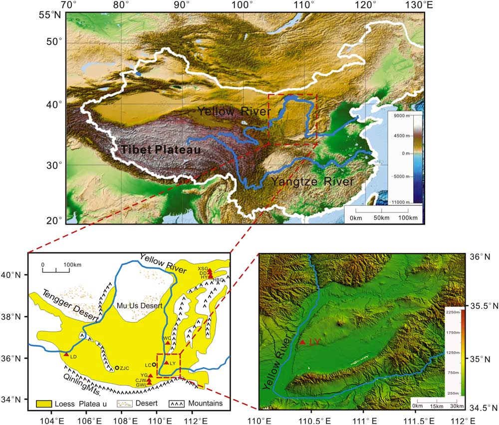
Figure 1 Map with Asian topography (modified from Li et al., Reference Li, Ao, Dekkers, Roberts, Zhang, Lin, Huang, Hou, Zhang and An2017), Chinese Loess Plateau (CLP; modified from Ao et al., Reference Ao, Roberts, Dekkers, Liu, Rohling, Shi, An and Zhao2016), Linyi section, and other faunal or section sites mentioned in the text. The red triangles and squares represent the faunal or section sites. CJW, Chenjiawo; DD, Daodi; GWL, Gongwangling; HBG, Huabaogou; HY, Hongya; LC, Luochuan; LD, Longdan; LY, Linyi; WC, Wucheng; XSG, Xiashagou; YG, Yangguo; ZJC, Zhaojiachuan. (For interpretation of the references to color in this figure legend, the reader is referred to the web version of this article.)
Starting from the early 1920s, a large number of faunal sites have been found on the CLP (Tong et al., Reference Tong, Li and Xie2008) (Fig. 1 and Tables 1 and 2). The Linyi Fauna is an important Early Pleistocene fauna that was found in the Yuncheng Basin, southeastern CLP, in 1959 and has yielded abundant mammalian fossils (Zhou and Zhou, Reference Zhou and Zhou1959, Reference Zhou and Zhou1965; Tang et al., Reference Tang, Zong and Xu1983). Although mammalian components suggest a broad age range within the Early Pleistocene (Zhou and Zhou, Reference Zhou and Zhou1959, Reference Zhou and Zhou1965; Tang et al., Reference Tang, Zong and Xu1983), its precise numerical age remains unknown. Here, we present a new paleomagnetic study that constrains the age of the Linyi Fauna. Combining previously dated Pleistocene faunas, we can establish the chronological sequencing of the mammalian faunas on the CLP.
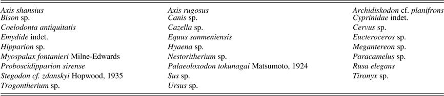
Table 1 List of the Linyi mammalian fauna (from Zhou and Zhou, Reference Zhou and Zhou1959, Reference Zhou and Zhou1965; Tang et al., Reference Tang, Zong and Xu1983).

Table 2 List of mammalian fauna directly dated by magnetostratigraphy on the Chinese Loess Plateau (Zhou and Zhou, Reference Zhou and Zhou1959, Reference Zhou and Zhou1965; Huang and Tang, Reference Huang and Tang1974; Wang, Reference Wang1982; Tang et al., Reference Tang, Zong and Xu1983; Cai, Reference Cai1987; Zhou et al., 1991; Qiu and Qiu, Reference Qiu and Qiu1995; Yue and Xue, Reference Yue and Xue1996; Zhang et al., Reference Zhang, Zheng and Liu2003; Cai et al., Reference Cai, Zhang, Zheng, Qiu and Li2004; Wang et al., Reference Wang, Løvlie, Yang, Pei, Zhao and Sun2005; Xue et al., Reference Xue, Zhang and Yue2006; Li et al., Reference Li, Zheng and Cai2008; Liu et al., Reference Liu, Deng, Li, Cai, Cheng, Yuan, Wei and Zhu2012). (For locations see Figure 1).

REGIONAL SETTING
At present, the Yuncheng Basin has a mean annual precipitation of 510 mm and a mean annual temperature of 13.5°C. Our studied Linyi section (35°07′29.5″N, 110°23′45.3″E) is located on the eastern bank of the Yellow River. It has a stratigraphic thickness of 170 m and consists of two parts: an overlying eolian Quaternary yellowish loess-paleosol sequence that consists of 15 layers of paleosol and 14 layers of loess (82 m) with underlying fluvial-lacustrine silty clay and sand (the so-called Sanmen Formation, ~88 m thick) that consists of 14 sand and silty clay packages. The Linyi Fauna occurs in a sand layer at a depth of 124–127 m below the top of the section (Fig. 2). The Linyi Fauna contains more than 30 mammal species, many of which are similar to other Early Pleistocene faunas in North China (Zhou and Zhou, Reference Zhou and Zhou1959, Reference Zhou and Zhou1965; Tang et al., Reference Tang, Zong and Xu1983). For example, the presence of Equus sanmeniensis, Hipparion sp., Proboscidipparion sirense, Cazella sp., and Ursus sp. (Tables 1 and 2) makes it comparable with the nearby Wucheng Fauna (1.2–1.9 Ma) (Yue et al., Reference Yue, Wang and Zheng1994, Reference Yue, Zhang, Deng and Zhang1998; Yue and Xue, Reference Yue and Xue1996). The presence of Equus sanmeniensis, Proboscidipparion sirense, Axis shansius, and Axis rugosus makes it comparable with the Yangguo Fauna (0.9–1.0 Ma) (Yue et al., Reference Yue, Wang and Zheng1994). The Wucheng and Yangguo locations are ~200 km north and southwest of the Yuncheng Basin, respectively.
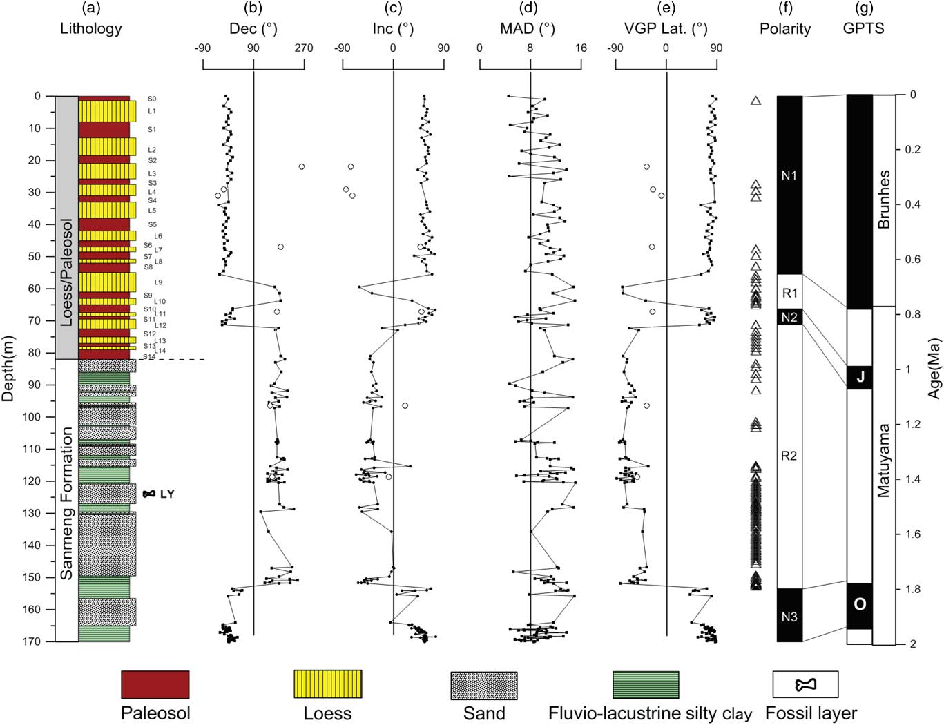
Figure 2 (color online) Magnetic polarity stratigraphy of the Linyi section. (a) Lithology. (b) Declination. (c) Inclination. (d) Maximum angular deviation (MAD). (e) Virtual geomagnetic pole (VGP) latitude. (f) Magnetic polarity sequence. (g) Geomagnetic polarity time scale (GPTS). Open circles represent rejected paleomagnetic data with inclinations <5° or paleomagnetic directions that are inconsistent with the expected geomagnetic field. Open triangles on the left-hand side of the polarity sequence represent rejected paleomagnetic data with unstable demagnetization trajectories at higher temperatures.
Sampling and methods
To obtain samples that were as fresh as possible, weathered surfaces were removed from the outcrop (at least the surface-most 20 cm). From the entire Linyi section, 98 oriented block samples were taken at 50–100 cm intervals from the loess-paleosol sequence, and 198 block samples were taken at 10−25 cm intervals from the underlying silty clay and sand succession. From each block sample, cubic (2 cm×2 cm× 2 cm) specimens were subsequently cut in the laboratory for stepwise thermal demagnetization analysis. In addition, 340 powdered samples were collected from the entire Linyi section for low-field magnetic susceptibility measurement (χ, calculated on a mass-specific basis), which is useful for establishing a time scale for the 82-m-thick loess-paleosol sequence.
The 340 powdered samples were packed into nonmagnetic cubic boxes (2 cm × 2 cm × 2 cm) for χ measurement with a Bartington Instruments MS2 magnetic susceptibility meter at 470 Hz. Temperature-dependent susceptibility (χ−T) and isothermal remnant magnetization (IRM) acquisition measurements were conducted on six powdered samples selected from various lithologies and magnetic polarity zones of the Linyi section. All the χ−T curves were measured in an argon atmosphere at a frequency of 976 Hz from room temperature up to 700°C and back to room temperature using an MFK1-FA Kappabridge instrument equipped with a CS-3 high-temperature furnace. The magnetic field during measurement was 300 A/m (peak to peak). To determine the temperature-dependent background susceptibility, a run with an empty furnace tube was performed before measuring the sediment samples. The susceptibility of each sediment sample was obtained by subtracting the measured background susceptibility (furnace tube correction) using the CUREVAL 5.0 program (AGICO, Czech Republic). The IRM acquisition curves were determined using an ASC IM-10-30 pulse magnetizer (capable of generating fields up to a maximum field of 2 T) and an AGICO JR-6A spinner magnetometer for remanence measurements. A total of 31 IRM steps were performed.
Stepwise thermal demagnetization was conducted using a 2G Enterprises Model 755-R cryogenic magnetometer installed in a magnetically shielded laboratory (with ambient field <150 nT). All samples were stepwise heated in 14 steps at 25–50°C increments to a maximum temperature of 580°C. After each demagnetization step, the remanent magnetization of each sample was measured. Demagnetization results were evaluated using orthogonal vector component diagrams (Zijderveld, Reference Zijderveld1967), and the principal component direction was computed using least-squares fitting (Kirschvink, Reference Kirschvink1980). The principal component analyses were conducted using the PaleoMag software developed by Jones (Reference Jones2002).
Results
Magnetic properties
Consistent with the ubiquitous occurrence of magnetite, all the heating curves are characterized by an inflection at ~585°C (Fig. 3). A steady χ increase from room temperature to ~300°C is possibly attributable to gradual unblocking of fine-grained ferrimagnetic particles or the release of stress upon heating (Van Velzen and Zijderveld, Reference Van Velzen and Zijderveld1995; Deng et al., Reference Deng, Zhu, Verosub, Singer and Vidic2004, Reference Deng, Shaw, Liu, Pan and Zhu2006; Liu et al., Reference Liu, Deng, Yu, Torrent, Jackson, Banerjee and Zhu2005, Reference Liu, Deng, Li and Zhu2010). A χ decrease at 300–500°C is generally interpreted as conversion of ferrimagnetic maghemite to weakly magnetic hematite (Florindo et al., Reference Florindo, Zhu, Guo, Yue, Pan and Speranza1999; Zhu et al., Reference Zhu, Deng and Jackson2001; Deng et al., Reference Deng, Zhu, Verosub, Singer and Vidic2004, Reference Deng, Shaw, Liu, Pan and Zhu2006) or changes in crystallinity, grain size, or morphology of the magnetic particles during heating (Dunlop and Özdemir, Reference Dunlop and Özdemir1997; Ao, Reference Ao2008; Ao et al., Reference Ao, Dekkers, Deng and Zhu2009, Reference Ao, Deng, Dekkers, Sun, Liu and Zhu2010). The cooling curves for six samples have much higher values than the corresponding heating curves, which indicates transformation of iron-containing clays or silicates to new ferrimagnetic minerals during heating (Hunt et al., Reference Hunt, Banerjee, Han, Solheid, Oches, Sun and Liu1995; Florindo et al., Reference Florindo, Zhu, Guo, Yue, Pan and Speranza1999; Zhu et al., Reference Zhu, Deng and Jackson2001; Ao et al., Reference Ao, Dekkers, Deng and Zhu2009).

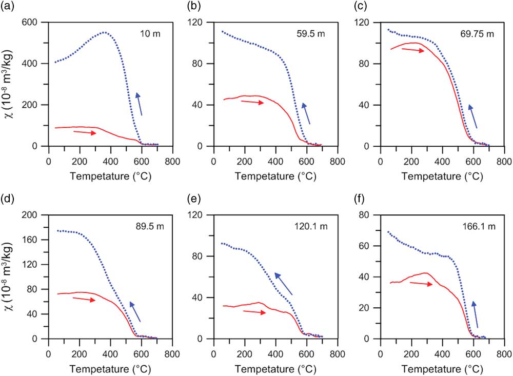
Figure 3 χ–T curves for six typical samples from the Linyi section. (a) 10 m (paleosol S1); (b) 59.5 m (loess L9); (c) 69.75 m (paleosol S11); (d) 89.5 m (silty clay); (e) 120.1 m (silty clay); (f) 166.1 m (silty clay). Red (blue) lines represent heating (cooling) curves. (For interpretation of the references to color in this figure legend, the reader is referred to the web version of this article.)
Consistent with the dominant contribution of magnetite to the magnetic mineralogy, all IRM acquisition curves undergo a major increase below 300 mT (Fig. 4). The additional slight increase in IRM after application of fields of >300 mT indicates the presence of high-coercivity hematite (Fig. 4).
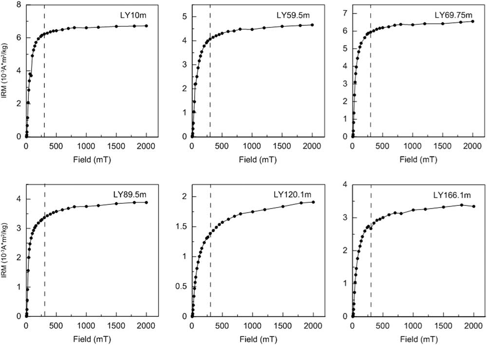
Figure 4 Isothermal remanent magnetization (IRM) acquisition curves for six typical samples from the Linyi section, the same levels as shown in Figure 3. The dashed vertical lines at 300 mT are shown to differentiate between low- and high-coercivity portions of the IRM acquisition curves.
Magneto-cyclostratigraphy
In most samples from the Linyi section, the natural remanent magnetization is composed of two components: (1) a secondary low-temperature component (LTC) isolated by progressive demagnetization to 150–250°C (occasionally up to 400°C) followed by (2) a characteristic remnant magnetization (ChRM) component isolated at higher temperatures (Fig. 5). The ChRM shows a relatively straightforward unidirectional trajectory toward the origin of orthogonal plots, while the LTC does not decay toward the origin for most samples. From the 296 demagnetized samples, there were 172 yield-stable ChRM components based on strict criteria: (1) data from at least four consecutive demagnetization steps were used for linear fitting, starting at least at 250°C; (2) a maximum angular deviation (MAD) <15° was required for the line fit; and (3) a calculated virtual geomagnetic pole (VGP) latitude >30° or <−30° (May and Butler, Reference May and Butler1986; Zhu et al., Reference Zhu, Deng and Pan2007; Ao et al., Reference Ao, An, Dekkers, Li, Xiao, Zhao and Qiang2013). The remaining 124 samples were excluded because they have unstable demagnetization trajectories, MAD values ≥15, VGP latitudes between –30° and 30°, or declinations trending roughly north (or south) but with upward (or downward) inclinations inconsistent with the expected field. Excluded samples tend to be associated with the fluvial-lacustrine interval that has a coarse-grained lithology of sand and silty clay (Fig. 2a). This might provide an explanation for the rather high proportion of excluded samples (42% of the total sample population). VGP latitudes calculated from all the 172 reliable ChRM directions are used to establish the magnetostratigraphic zonation, which allows identification of three normal and two reversed polarity zones (Fig. 2). Each polarity zone is defined based on at least two consecutive VGP latitudes of identical polarity. Correlation of the Linyi magnetic polarity sequence to the geomagnetic polarity time scale (Hilgen et al., Reference Hilgen, Lourens and van Dam2012) suggests that the Linyi section records the Brunhes chron, Jaramillo and Olduvai subchrons, and successive reverse polarity portions of the intervening Matuyama chron (Figs. 2 and 6).
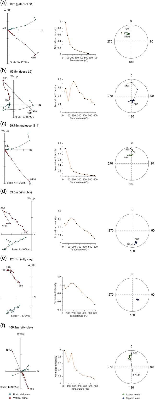
Figure 5 Demagnetization diagrams for stepwise thermal demagnetization of the natural remanent magnetization (NRM) data, their decay curves (plots in the second column), and corresponding equal-area stereographic projections (rightmost plots) for selected samples from the Linyi section (the same samples as in Figs. 3 and 4). (a) 10 m (paleosol S1); (b) 59.5 m (loess L9); (c) 69.75 m (paleosol S11); (d) 89.5 m (silty clay); (e) 120.1 m (silty clay); (f) 166.1 m (silty clay). Green and red circles in the orthogonal projections represent horizontal and vertical planes, respectively. Green and blue circles in the equal-area stereographic projections are mean lower hemis and upper hemis. The numbers refer to the temperatures in degrees Celsius. (For interpretation of the references to color in this figure legend, the reader is referred to the web version of this article.)
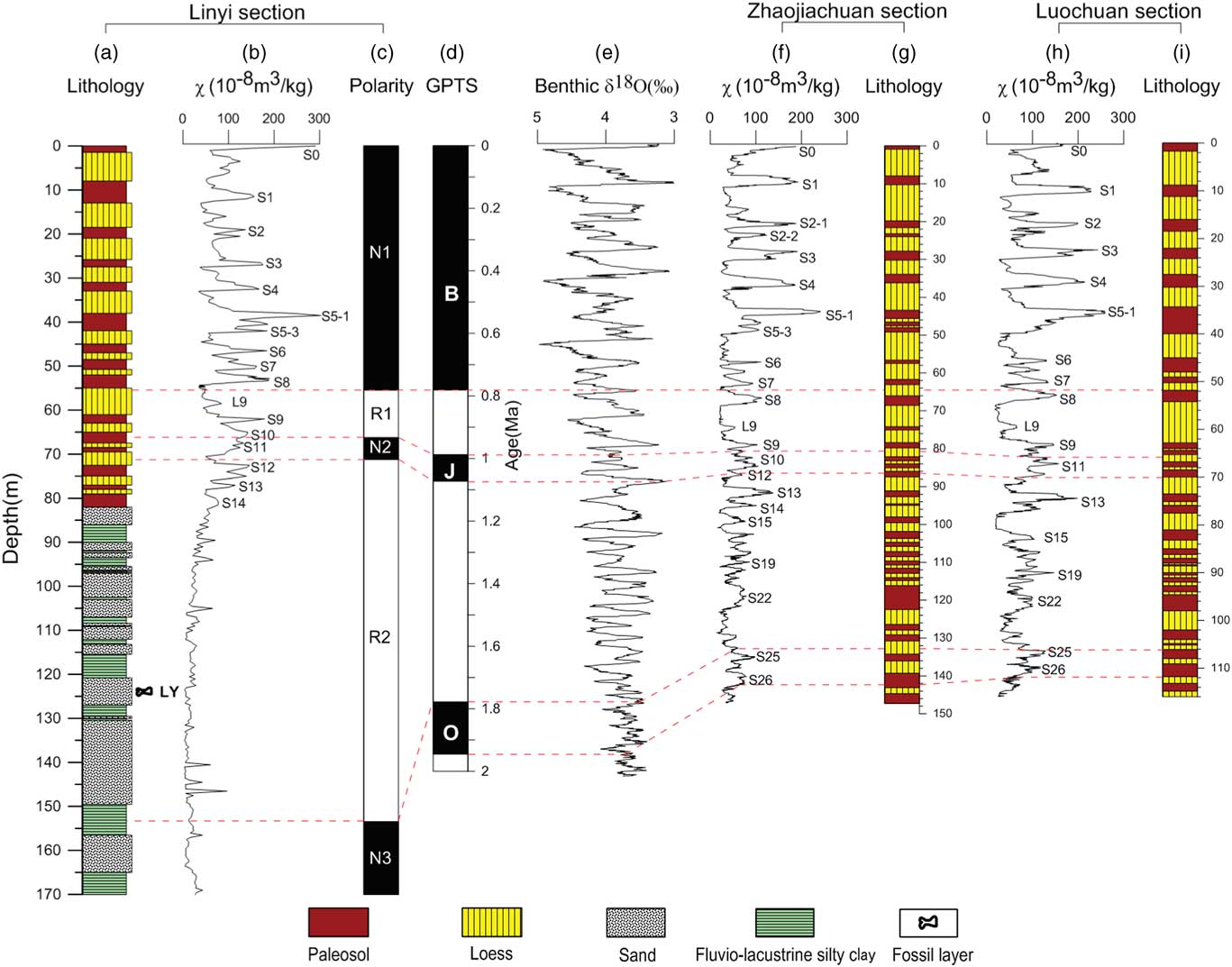
Figure 6 (color online) Lithostratigraphy, magnetic susceptibility stratigraphy, and magnetostratigraphy for the Linyi, Zhaojiachuan (Sun et al., Reference Sun, Clemens, An and Yu2006), and Luochuan (Liu, Reference Liu1985; Lu et al., Reference Lu, Liu, Zhang, An and Dodson1999) sections and correlations to the geomagnetic polarity time scale (GPTS) (Hilgen et al., Reference Hilgen, Lourens and van Dam2012) and benthic δ18 O (‰) (Zachos et al., Reference Zachos, Pagani, Sloan, Thomas and Billups2001). (a) Lithology of Linyi section. (b) Magnetic susceptibility of Linyi section. (c) Magnetic polarity sequence of Linyi section. (d) Geomagnetic polarity time scale (GPTS). (e) Benthic δ18 O (‰). (f) Magnetic susceptibility of Zhaojiachuan section. (g) Lithology of Zhaojiachuan section. (h) Magnetic susceptibility of Luochuan section. (i) Lithology of Luochuan section.
Consistent with the lithological transition from fluvial-lacustrine silty clay and sand sequence to the overlying eolian loess-paleosol sequence, the χ is shifted from low to high values (Fig. 6a and b). The χ for the fluvial-lacustrine silty clay and sand sequence (82–170 m) ranges from ~3 × 10⁻⁸ m3/kg to ~100 × 10−8 m3/kg, with an average of ~30 × 10−8 m3/kg. The χ for the overlying loess-paleosol sequence (0–82 m) ranges from ~30 × 10−8 m3/kg in loess to ~300 × 10−8 m3/kg in some paleosols; such values are typical of Pleistocene loess-paleosol sequences from the CLP (Wang et al., Reference Wang, Løvlie, Yang, Pei, Zhao and Sun2005; Liu et al., Reference Liu, Jin, Hu, Jiang, Ge and Roberts2015). Loess and paleosol layers are characterized by low and high χ, respectively. Temporal loess-paleosol χ variability of the Linyi section is closely correlated with that of other sections across the CLP, such as those at nearby Zhaojiachuan (Sun et al., Reference Sun, Clemens, An and Yu2006) and Luochuan (Liu, Reference Liu1985; Lu et al., Reference Lu, Liu, Zhang, An and Dodson1999) sections (Fig. 6). In particular, the composite paleosol S5 with unusually high χ and redder color and loess L9 with extremely coarse grain sizes, which are important marker layers in the Chinese loess-paleosol sequence (Liu, Reference Liu1985), are clearly identified in the mid-Brunhes and prior to the Matuyama-Brunhes boundary in the Linyi section, respectively (Fig. 6). Based on this correlation, we found that the 82-m-thick Linyi loess-paleosol sequence ranges continuously from paleosol S0 to S14. The top paleosol is S0, which formed during the present interglacial period (Sun et al., Reference Sun, Clemens, An and Yu2006).
Discussion
The lithological and χ cycles of loess-paleosol sequences can be correlated from section to section across the CLP as well as cycle by cycle to benthic δ18O records (Kukla et al., Reference Kukla, Heller, Liu, Xu, Liu and An1988; An et al., Reference An, Kukla, Porter and Xiao1991; Heslop et al., Reference Heslop, Langereis and Dekkers2000; Ding et al., Reference Ding, Derbyshire, Yang, Yu, Xiong and Liu2002; Sun et al., Reference Sun, Clemens, An and Yu2006). At the Linyi section, the lithological and χ records indicate that the 82-m-thick loess-paleosol sequence continuously spans from paleosol layers S0 to S14 (Fig. 6), covering the past 1.26 Ma (Sun et al., Reference Sun, Clemens, An and Yu2006). Brunhes chron, Jaramillo and Olduvai subchrons, and successive reverse polarity portions of the intervening Matuyama chron are successfully identified in the Linyi section (Fig. 6). The Brunhes-Matuyama boundary is identified in S8 in the Linyi section, while the Jaramillo polarity subchron is identified in S10–L12. The termination of the Olduvai polarity subchron is identified at a depth of 153.4 m in the underlying fluvial-lacustrine sequence.
There are two potential age estimates for the Linyi Fauna. The first option yields an age of ~1.52–1.55 Ma for the Linyi Fauna, which is obtained via linear interpolation between Olduvai and Jaramillo polarity subchrons, assuming a constant long-term sedimentation rate between them. The eolian loess-paleosol sequence (71.25–82 m) prior to the Jaramillo polarity subchron should have a lower sedimentation rate than the underlying fluvial-lacustrine silty clay and sand sequence (82–153.4 m) above the Olduvai polarity subchron. Assuming a constant sedimentation rate for the overlying eolian Quaternary yellowish loess-paleosol sequence and the underlying fluvial-lacustrine silty clay and sand sequence may have caused this age estimate to be slightly younger. The second yields an age of ~1.56–1.58 Ma, which is established by linear interpolation using the bottom age of paleosol S14 (Sun et al., Reference Sun, Clemens, An and Yu2006) and the top age of the Olduvai subchron (Hilgen et al., Reference Hilgen, Lourens and van Dam2012) as constraints. The bottom of paleosol S14 has an age of 1.26 Ma as suggested by tuning the grain-size record to orbital obliquity and precession parameters (Sun et al., Reference Sun, Clemens, An and Yu2006). Considering the possible presence of unobservable small hiatuses and variations in sedimentation rate for the sand and silty clay deposits in the fluviolacustrine sequence, we suggest an age of 1.5–1.6 Ma for the Linyi Fauna.
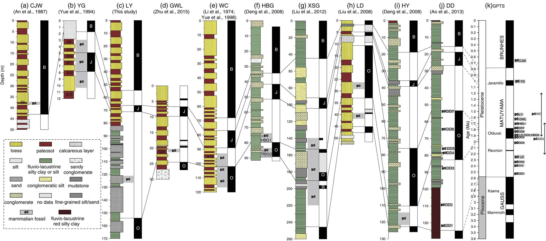
Combining our new and previous paleomagnetic dating of faunas, we can now establish a magnetochronological framework for the faunas on the CLP. The previously published magnetostratigraphic data (Li et al., Reference Li, An and Wang1974; An et al., Reference An, Liu, Kan, Sun, Wang, Kao, Zhu and Wei1987; Yue et al., Reference Yue, Wang and Zheng1994; Deng et al., Reference Deng, Zhu, Zhang, Ao and Pan2008; Liu et al., Reference Liu, Zhang, Han and Liu2008, Reference Liu, Deng, Li, Cai, Cheng, Yuan, Wei and Zhu2012; Ao et al., Reference Ao, An, Dekkers, Li, Xiao, Zhao and Qiang2013) have suggested that the faunas of DD, HY, LD, XSG, HBG2, HBG1, WC, GWL, LY, and YG reside in the Matuyama chron, with only CJW in the Brunhes (Fig. 7; see figure caption for definition of abbreviations). More precisely, the DD Fauna appears to be located between the Gauss-Matuyama boundary and the termination of the Olduvai polarity subchron, ranging in age from ca. 2.5 to 1.8 Ma (Ao et al., Reference Ao, An, Dekkers, Li, Xiao, Zhao and Qiang2013); LD Fauna has two mammal fossil layers, which occur during the early the Olduvai subchron and pre-Olduvai Matuyama chron, yielding an age between 2.25 and 1.9 Ma (Liu et al., Reference Liu, Zhang, Han and Liu2008) (Fig. 7). The HY Fauna is located within the earliest Matuyama chron, with an age of 2.4 Ma. The XSG Fauna is located between the pre-Reunion Matuyama chron and the post-Olduvai Matuyama chron, with an age of 1.7–2.2 Ma. The HBG2 Fauna is located within the lower Olduvai polarity subchron, with an estimated age of ca 1.9 Ma, while the HBG1 Fauna occurs later than the termination of the Olduvai polarity subchron, with an estimated age of ca 1.7 Ma (Deng et al., Reference Deng, Zhu, Zhang, Ao and Pan2008). The WC Fauna is located within the middle Matuyama chron, with an estimated age of ca. 1.2–1.9 Ma (Li et al., Reference Li, An and Wang1974; Yue et al., Reference Yue, Wang and Zheng1994, Reference Yue, Zhang, Deng and Zhang1998). The GWL Fauna occurs during S22 or S23 of the Chinese loess-paleosol sequence, with an age of 1.54–1.65 Ma (Zhu et al., Reference Zhu, Dennell, Huang, Wu, Rao, Qiu and Xie2015). The CJW Fauna corresponds to S6 based on the biochronology and stratigraphic correlation with typical loess-paleosol sequences of Luochuan, yielding an age of ~0.65 Ma (An et al., Reference An, Liu, Kan, Sun, Wang, Kao, Zhu and Wei1987; An and Kun, Reference An and Kun1989) (Fig. 7). The YG Fauna occurs around the Jaramillo subchron, with an age of 0.98–1.05 Ma (Yue et al., Reference Yue, Wang and Zheng1994). Therefore, our established magnetochronological framework indicates that the CLP faunas range from ca 2.5 to 0.6 Ma, spanning most of the Pleistocene, with significantly flourishing faunas during the Early and Middle Pleistocene (Fig. 7).

Figure 7 (color online) A synthetic diagram relating the magnetostratigraphically dated sections on the Chinese Loess Plateau, which contain the mammalian fauna sites, to the geomagnetic polarity time scale (GPTS). CJW, Chenjiawo; DD, Daodi; GWL, Gongwangling; HBG, Huabaogou; HY, Hongya; LD, Longdan; LY, Linyi; WC, Wucheng; XSG, Xiashagou; YG, Yangguo. (a) Lithology, Depth of fauna and Magnetic polarity sequence of CJW section. (b) Lithology, Depth of fauna and Magnetic polarity sequence of YG section. (c) Lithology, Depth of fauna and Magnetic polarity sequence of LY section. (d) Lithology, Depth of fauna and Magnetic polarity sequence of GWL section. (e) Lithology, Depth of fauna and Magnetic polarity sequence of WC section. (f) Lithology, Depth of fauna and Magnetic polarity sequence of HBG section. (g) Lithology, Depth of fauna and Magnetic polarity sequence of XSG section. (h) Lithology, Depth of fauna and Magnetic polarity sequence of LD section. (i) Lithology, Depth of fauna and Magnetic polarity sequence of HY section. (j) Lithology, Depth of fauna and Magnetic polarity sequence of DD section. (k) Geomagnetic polarity time scale (GPTS).
The abundant faunas on the CLP contain both typical grassland and woodland species (Tables 1 and 2 indicate that mixed grassland and woodland habitats were prevalent during the Pleistocene). For these well-dated faunas, we further calculated the occurrence of woodland and grassland mammalian groups as percentages (Fig. 8). Overall, grassland mammals have higher percentages than woodland mammals in these faunas, which is consistent with the semiarid CLP environment during the Pleistocene (Liu, Reference Liu1985; Maher, Reference Maher2016), under the influence of global glacial-interglacial cycles (Figs. 2 and 6).
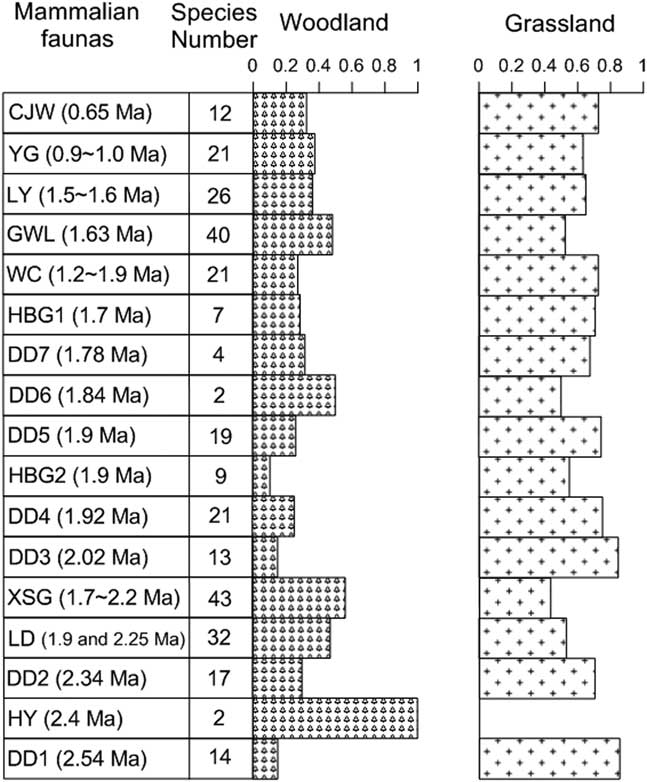
Figure 8 Variability of the total number of mammalian species and percentages of grassland and woodland groups for the well-dated Pleistocene faunas on the Chinese Loess Plateau. CJW, Chenjiawo; DD, Daodi; GWL, Gongwangling; HBG, Huabaogou; HY, Hongya; LD, Longdan; LY, Linyi; WC, Wucheng; XSG, Xiashagou; YG, Yangguo.
Conclusions
An integrated stratigraphic analysis, involving lithostratigraphy, magnetic susceptibility stratigraphy, and magnetostratigraphy, indicates that the Linyi section records a polarity pattern from the Brunhes chron to the Olduvai subchron. The Linyi Fauna’s layer occurs in a reversed polarity magnetozone between the Olduvai and Jaramillo subchrons, yielding an estimated age of ~1.5–1.6 Ma. Combining our new and previous magnetostratigraphic dating of faunas, we establish a Pleistocene magnetochronology spanning from 2.54 to 0.65 Ma for the faunas on the CLP.
ACKNOWLEDGMENTS
We are grateful to Randall Schaetzl for his suggestions that improved the paper and PhD student Yang Yi from the Nanjing Institute of Geology and Palaeontology, Chinese Academy of Sciences for help in sampling and experiments. Thank you for the comments provided by the editors and two reviewers. This work was supported financially by the National Natural Science Foundation of China (grant 41372020) and the Key Research Program of Frontier Sciences, Chinese Academy of Sciences (grants QYZDB-SSW-DQC021, QYZDY-SSW-DQC001, and ZDBS-SSW-DQC001).