INTRODUCTION
One of the fundamental relationships within Earth systems is the interaction between the geosphere and the biosphere. The role of terrestrial plants in shaping newly formed landscapes (i.e., primary succession) has been studied after glacial retreat (Buma et al., Reference Buma, Bisbing, Krapek and Wright2017), volcanic eruptions (Cutler et al., Reference Cutler, Belyea and Dugmore2008), and mass movement (Colombaroli and Gavin, Reference Colombaroli and Gavin2010). Most Earth surfaces are considered to undergo relatively slow rock weathering processes. These processes are dominated by climatic factors, but vegetation also influences weathering (Pawlik et al., Reference Pawlik, Phillips and Samonil2016) and vice versa (Hahm et al., Reference Hahm, Riebe, Lukens and Araki2014). The nature of the geosphere-biosphere relationship, and its spatial and temporal regulators, vary across various climatic, geomorphic, tectonic, and biotic settings (Porder, Reference Porder2014). Here, we focus on the biotic setting, comparing the pace and nature of ecosystem development between two major vegetation types—forest and grassland—to improve our understanding of the relative effect of biota on the geochemical composition of sediments over millennial timescales (Jenny, Reference Jenny1941).
To understand landscape development over time, we are often limited to comparing Earth surface features to source rock material. While this can give some indication of how plants may have interacted with rock on timescales of 105 or 106 yr, the intermediate steps, rates, and controls of geosphere-biosphere processes are unknown using this approach. Nonetheless, chronosequence studies of primary succession have demonstrated, broadly, how ecosystems change over time. As primary successional stages develop, there is generally a temporal sequence of biogeochemical changes such as base cation mineral weathering, organic matter accumulation from the terrestrial biosphere, increases in plant-available nitrogen, and decreases in phosphorus (Laliberte et al., Reference Laliberte, Turner, Costes, Pearse, Wyrwoll, Zemunik and Lambers2012; Wardle et al., Reference Wardle, Walker and Bardgett2004). However, characterizations of these early stages lack high temporal detail. In particular, we may be missing important system behavior such as tipping points and pedogenic thresholds (Vitousek and Chadwick, Reference Vitousek and Chadwick2013).
Early postglacial successional processes can be reconstructed by studying geochemical records of rock-plant interactions in continuously deposited lacustrine sedimentary records (Mackereth, Reference Mackereth1966; Pennington et al., Reference Pennington, Haworth, Bonny and Lishman1972; Engstrom and Hansen, Reference Engstrom and Hansen1985). These records provide information on a finer scale (<17,000 yr BP) than is possible in temperate chronosequences. Measuring elemental concentrations in sedimentary sequences has a long history (Likens, Reference Likens1985; Willis et al., Reference Willis, Braun, Sumegi and Toth1997) but, because of the proxy nature of these records, interpretation is aided by a multitude of other parameters describing the properties of these systems (Kylander et al., Reference Kylander, Ampel, Wohlfarth and Veres2011). Of particular importance are proxies of transport processes from the catchment to the sediment. These dynamic processes are a function of climatic changes, lithological variability, and differences in vegetation cover between grassland and forested catchments. Through multi-proxy investigation, sedimentary sequences have begun to yield unique information about early ecosystem processes. For example, important information about P cycling can be obtained from studying the chemical weathering of the phosphate mineral apatite early in catchment development (Boyle, Reference Boyle2007; Norton et al., Reference Norton, Perry, Saros, Jacobson, Fernandez, Kopacek, Wilson and SanClements2011).
There are several potential mechanisms for how terrestrial vegetation could determine trajectories of biogeochemical change on centennial to millennial timescales, as seen in Holocene sedimentary records. First, vegetation composition can influence chemical weathering rates. There are examples of organic acids produced by coniferous vegetation speeding ecosystem acidification (Ford, Reference Ford1990) and even leading to podsolization during the Holocene (Davis et al., Reference Davis, Anderson, Dixit, Appleby and Schauffler2006). Conversely, removal of trees has been demonstrated to cause an increase in soil pH (Bradshaw et al., Reference Bradshaw, Rasmussen and Odgaard2005). Second, the degree of vegetation cover (primary productivity) can affect hydrologic pathways and physical weathering. Large-scale changes from grassland to forests between stadials and interstadials during the last glacial, with different rates of productivity, led to differences in weathering product delivery to a depositional basin (Kylander et al., Reference Kylander, Ampel, Wohlfarth and Veres2011). Finally, there are also potential feedbacks between fire regimes and geochemistry. In lodgepole pine forests of the western United States, loss of nitrogen and base cations has occurred over the past 4000 yr with repeated fire (Dunnette et al., Reference Dunnette, Higuera, McLauchlan, Derr, Briles and Keefe2014; Leys, Reference Leys, Higuera, McLauchlan and Dunnette2016). While fire events and plant cover were significantly related at Thyl Lake in the French Alps, soil processes were primarily linked to vegetation composition and secondarily to changes in fire regime (Mourier et al., Reference Mourier, Poulenard, Carcaillet and Williamson2010).
To assess rates, patterns, and mechanisms of ecosystem development after glacial retreat, we compared two sedimentary sequences in the upper Midwestern United States from a grassland site and a forested site. Our three main questions were: (1) How did source material change over the sedimentary sequences? (2) What were the patterns of nutrients, especially limiting nutrients such as nitrogen, potassium, calcium, and magnesium, during Holocene ecosystem development? (3) Did the terrestrial biosphere determine the trajectory of elemental change at each site?
METHODS
Study sites
Fox Lake is located in southern Minnesota, USA, has a surface area of 3.85 km2, and a maximum water depth of 6 m. The lake was formed during the retreat of the Des Moines Lobe of the Laurentide Ice Sheet at the end of the last glaciation about 12,000 yr (Maher, Reference Maher1982; Lusardi et al., Reference Lusardi, Jennings and Harris2011). Fox Lake is approximately 10 km from the southernmost extent of the Des Moines Lobe, but the timing and path of deglaciation are not entirely clear in this region. The catchment parent material is calcareous glacial till, and lake water geochemistry is dominated by catchment input rather than precipitation-evaporation dynamics (Gorham et al., Reference Gorham, Dean and Sanger1983). There is one small inlet stream on the west side of the lake. Soils surrounding Fox Lake are a mix of Udols and Aquolls—poor to well-drained clay loams formed from calcareous tills—and are often deep (>2m; USDA NRCS, 2018).
Devils Lake is located in southern Wisconsin, has a surface area of 1.53 km2, and a maximum depth of 14 m. Catchment parent material is primarily hematite-rich quartzite, as well as glacial till deposited in moraines from the Green Bay Lobe at the end of the last glacial period, ca. 18,500 cal yr BP (Attig et al., Reference Attig, Hanson, Rawling, Young and Carson2011). Soils in this area are thin (0.5–1 m) Udalfs—moderately well-drained stony and cobbly silt loams formed from a mixture of loess and quartzite bedrock (USDA NCRS, 2018). Devils Lake is located just to the south of the maximum extent of the Laurentide Ice Sheet. The catchment of Devils Lake has areas of quartzite cliffs and the geology is considerably different than Fox Lake and therefore these two sites capture a wide range of weathering products to lakes.
The two study sites are ~480 km apart (Fig. 1). The sites were chosen due to their positions relative to the furthest advance of the Laurentide Ice Sheet and dominant vegetation cover during the Holocene. At the time of Euro-American settlement (mid-1800s), Fox Lake was tallgrass prairie characterized by warm-season grass species such as Andropogon gerardii, Sorghastrum nutans, and Schizachyrium scoparium (Küchler, Reference Küchler1964). Today, the Fox Lake catchment is dominated by agriculture. In contrast, Devils Lake is surrounded by mixed deciduous-coniferous forest including the conifer Pinus strobus, deciduous components of Quercus rubra, Quercus alba, and Acer rubrum, and herbaceous savanna understory vegetation. Modern vegetation between the two sites likely varies due to differences in precipitation. Devils Lake on average receives 914–940 mm of annual precipitation, while Fox Lake receives 762–812 mm of annual precipitation (NOAA, 2018).
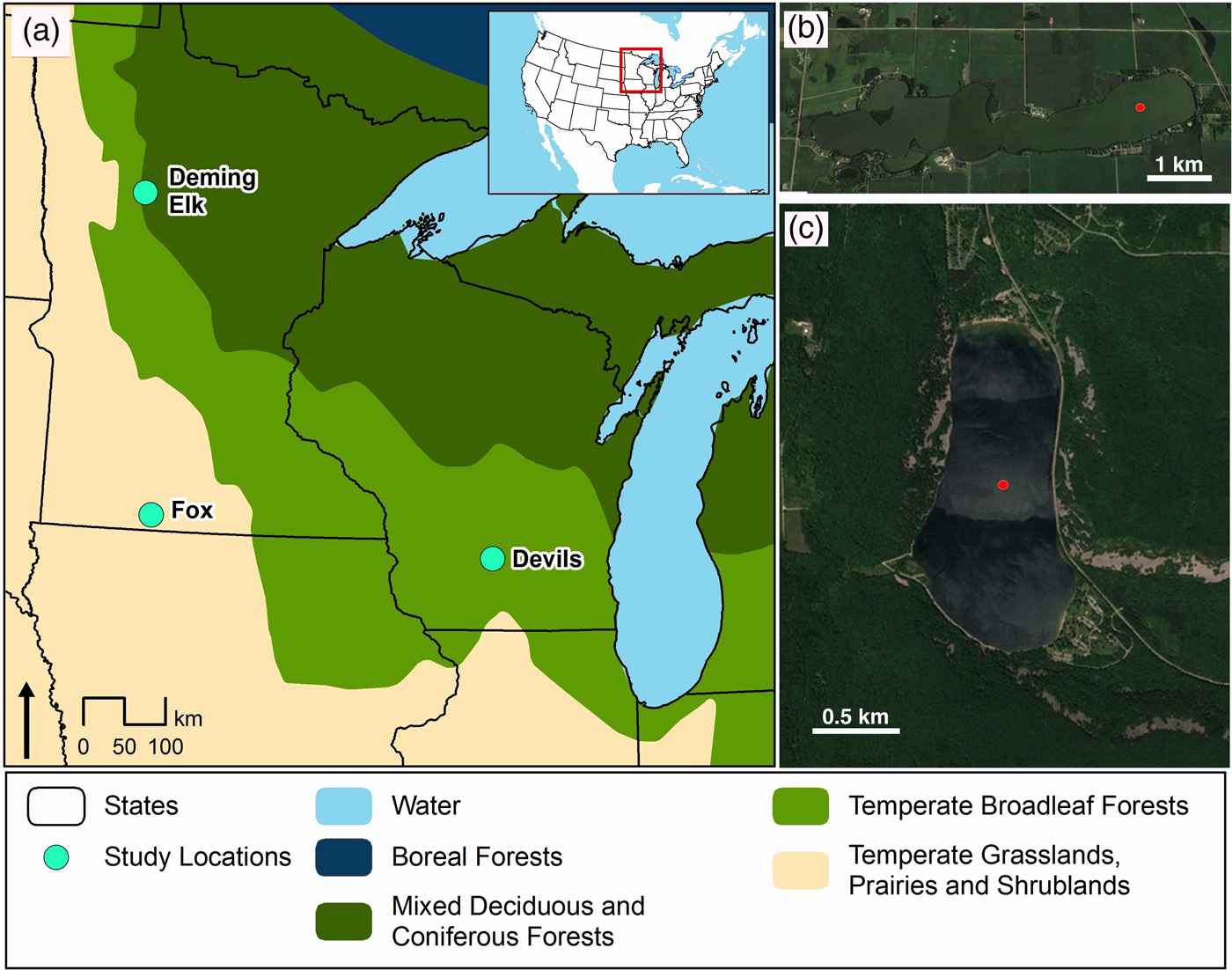
Figure 1. (a) Regional map with locations of Fox Lake, Devils Lake, and the other sites referred to in text (Deming Lake AND Elk Lake). (b) Detail of Fox Lake basin morphology and vegetation. (c) Detail of Devils Lake basin morphology and vegetation. Red dots represent coring sites. (For interpretation of the references to color in this figure legend, the reader is referred to the web version of this article.)
In February 2012, we obtained sediment cores from both Devils Lake and Fox Lake using piston corers. The Fox Lake sediment core was 9.3 m long and the Devils Lake sediment core was 10.4 m long.
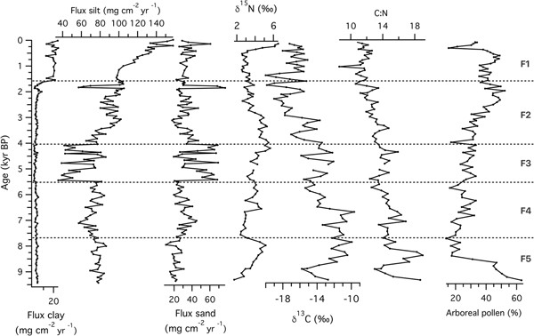
A previous study of Fox Lake established a radiocarbon-based chronology as well as the vegetation and fire history (Commerford et al., Reference Commerford, Leys, Mueller and McLauchlan2016). The same sediment cores were used to measure the proxies described in the current manuscript. Previously, vegetation history reconstructed by pollen analysis from 9300 cal yr BP indicates that Fox Lake has been a grassland site since near the beginning of the record, with only one slight change from oak forest to grassland at 8200 cal yr BP (Commerford et al., Reference Commerford, Leys, Mueller and McLauchlan2016). The oak forest vegetation is characterized by high amounts of Quercus pollen (an arboreal pollen type), and the grassland vegetation is characterized by high amounts of non-arboreal pollen types such as Poaceae, Ambrosia, and Artemisia. Thus, for this study we used the % arboreal pollen to capture this vegetation transition at Fox Lake. The lithostratigraphy for Fox Lake is consistently characterized by dark brown, high organic matter sediment throughout the core. Five zones (F1–F5) were determined with constrained hierarchical cluster analysis using changes in magnetic susceptibility (Commerford et al., Reference Commerford, Leys, Mueller and McLauchlan2016).
Details of the lithology, radiocarbon chronology, fire history, and geochemical proxy records of Devils Lake are also described previously (Williams et al., Reference Williams, McLauchlan, Mueller, Mellicant, Myrbo and Lascu2015). The same sediment cores were used to measure the proxies described in the current manuscript. Devils Lake has a much longer record than Fox Lake, beginning at 17,000 cal yr BP (Williams et al., Reference Williams, McLauchlan, Mueller, Mellicant, Myrbo and Lascu2015), and captures three types of forest: spruce, pine, and hardwood (Maher, Reference Maher1982). The detailed pollen stratigraphy with three forest types was established by Maher (Reference Maher1982) and Williams et al. (Reference Williams, McLauchlan, Mueller, Mellicant, Myrbo and Lascu2015) established a robust chronology with input from Grimm et al. (Reference Grimm, Maher and Nelson2009). The changes in vegetation from coniferous to hardwood forest types are characterized by changes in spruce pollen (Picea), pollen from hardwood trees (Quercus and Ulmus), and grass pollen (Poaceae). The lithostratigraphy of Devils Lake varies throughout the core, with five main zones. Five zones (D1–D5) were delineated based on sediment appearance, composition, and mineralogy (Williams et al., Reference Williams, McLauchlan, Mueller, Mellicant, Myrbo and Lascu2015).
The two study sites differ in multiple ways—they cover different time periods (one starting in the late glacial and the other in the Early Holocene), are situated in different geologic terrains, and were analyzed for a different suite of sedimentary proxies—but chiefly provide an important contrast in dominant vegetation type and the degree of vegetation change during their respective records. To put the lithologic, pollen, and sedimentological changes for each lake in context, we use the stratigraphic zones previously delineated and published for each lake (Fox Lake in Commerford et al. [Reference Commerford, Leys, Mueller and McLauchlan2016] and Devils Lake in Williams et al. [Reference Williams, McLauchlan, Mueller, Mellicant, Myrbo and Lascu2015]). The same sediment cores were used to establish the stratigraphic zones and also for the new analyses presented in this manuscript for both Fox Lake and Devils Lake (Table 1).
Micro X-ray fluorescence (μ-XRF) core scanning
All sections of the Devils Lake and Fox Lake sediment cores were scanned using an Itrax XRF core scanner (Cox Analytical Systems, Gothenburg, Sweden) at the LacCore X-ray Fluorescence Laboratory housed at the University of Minnesota Duluth Large Lakes Observatory. This instrument produces an optical RBG digital image, a microradiographic digital image, and count data for most elements from aluminum (atomic number 13) to uranium (92). XRF scans were performed using a molybdenum tube set at 30 kV and 25 mA with a dwell time of 60 s and a step size of 10 μm. The Fox Lake data were reduced by averaging to 1 cm, while the Devils Lake data were averaged to 0.1 cm and then smoothed using a 10-point running mean. The raw count data is expressed as counts/second (cps).
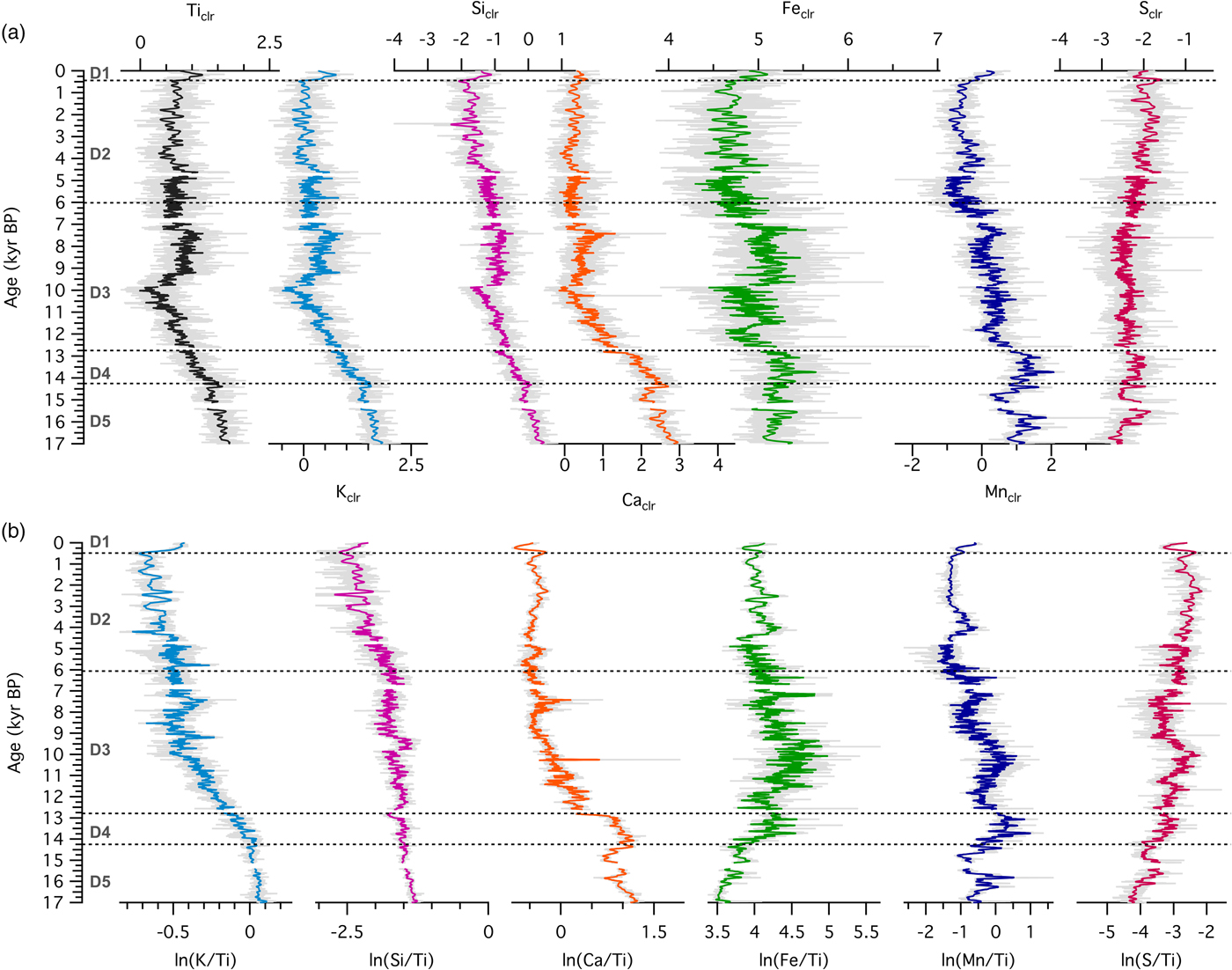
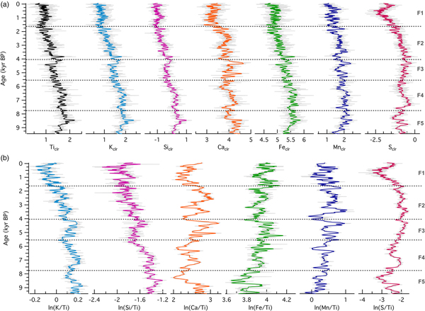
For elements with sufficient counts, we divided the elemental counts by molybdenum coherence (MoCoh) values for each measured interval to account for variation among analytical time periods in the characteristics of the Mo tube. A centered-log ratio (clr) transformation was then performed on the MoCoh-corrected μ-XRF intensities, such that I clr = ln(I/G), where I is the intensity of the element transformed, and G is geometric mean of all the elements analyzed at the same measuring point. We analyzed a set of selected elements that had sufficient counts, and that are important in ecosystem and weathering processes. Although the investigated elements are found in various compounds in the sediment, they can indicate three types of processes: allochthonous, biogenic, and authigenic (Lopez et al., Reference Lopez, Navarro, Marce, Ordoñez, Caputo and Armengol2006). We used Ticlr and Kclr as indicative of detrital input; Siclr and Caclr as indicative of detrital input, as well as biogenic silica and calcite formation, respectively; and Feclr, Mnclr, and Sclr as indicative in part of detrital input, as well as redox processes.
To better trace these additional processes, MoCoh standardized values were then divided by Ti counts to obtain a measure of silicate weathering (K/Ti), biogenic silica (Si/Ti), and authigenic mineral precipitation (Ca/Ti, Fe/Ti, Mn/Ti, and S/Ti). While none of these elements should be interpreted as uniformly indicating a single process, their variability as assemblages may lead to an improved understanding of lake sedimentation (Martin-Puertas et al., Reference Martin-Puertas, Tjallingii, Bloemsma and Brauer2017). In conjunction with other proxies, elemental assemblages can be used to assess catchment inputs (both lithological and organic), redox conditions, and potentially aquatic primary productivity. Elemental concentrations are sometimes non-linearly correlated with XRF intensities throughout sediment cores, due to matrix effects, physical properties, and geometry of the sample in different sections. To avoid such effects, we resort to using log ratios of μ-XRF intensities, which are linear functions of log ratios of element concentrations (Weltje and Tjallingii, Reference Weltje and Tjallingii2008). The log-ratio transformation also helps with issues related to closed-sum data encountered in multivariate statistical analyses (Martin-Puertas et al., Reference Martin-Puertas, Tjallingii, Bloemsma and Brauer2017).
Stable isotope analysis
Organic carbon (C) and nitrogen (N) concentrations and standard isotopic ratios (δ13C, δ15N) were measured on dried bulk sediment samples every 10 cm for the Fox Lake sediment core and every 5 cm for the Devils Lake sediment cores. Analyses were conducted at the Stable Isotope Mass Spectrometry Laboratory at Kansas State University and the Central Appalachian Stable Isotope Facility at the University of Maryland following standard procedures for sediment samples. To maximize precision, in-house standards calibrated to PeeDee Belemnite (δ13C) and atmospheric N2 gas (δ15N) were used. Analytical error was better than 0.1‰ for δ13C and better than 0.2‰ for δ15N. The C:N ratio of the bulk sediment was calculated by dividing %C by %N.
Particle size analysis
Bulk sedimentary particle size was measured for Fox Lake sediments because of an expectation that particle size would change during the Holocene as aridity and eolian inputs changed. We did not measure particle size with this method at Devils Lake because of the nature of the sedimentary material and difficulty in interpreting bulk particle size in this depositional environment. Throughout the 9.3-m Fox Lake sediment core, 1 mL samples were removed from every third centimeter. Each sample was pretreated with 30 mL of 25% H2O2 at 80°C to remove organic matter. After settling overnight, excess liquid was decanted. Samples were measured using a laser particle size analyzer through a wet dispersion unit (Mastersizer 3000 and Hydro EV accessory; Malvern Instruments, Worcestershire, UK). The analyzer outputted volume percentages for 100 size classes from 0.01 to 3500 μm. Volume percentages from these size classes were summed according to United States Department of Agriculture (USDA) grain size categories: clay <2 μm; silt, 2–50 μm; sand, 50–2000 μm; and gravel, >2000 μm. While most sediments are finer-grained than soils, we used the USDA classification to match interpretations of particle size transport.
Magnetic parameters and unmixing model
To gain insight into sediment dynamics at Devils Lake we calculated the fluxes of lithogenic (LITH), pedogenic (PED), and biogenic (BIO) magnetic minerals using the method developed by Lascu et al. (Reference Lascu, Banerjee and Berquo2010). For this we measured anhysteretic remanent magnetization (ARM), saturation magnetization (Ms), and saturation remanent magnetization (Mrs) at the Institute for Rock Magnetism, University of Minnesota. A D-Tech 2000 demagnetizer was used for the acquisition of ARM in a 0.1 mT direct field superimposed on an alternating frequency field decaying at a rate of 5 μT per half cycle from a peak value of 200 mT. ARM susceptibility (χARM) was calculated by dividing the ARM to the direct field. Remanence measurements were performed using a 2G superconducting rock magnetometer. Ms and Mrs were obtained from slope-corrected hysteresis loops measured on a Princeton Measurements vibrating sample magnetometer using a maximum applied field of 1 T and a step size of 5 mT.
Using the unmixing model of Lascu et al. (Reference Lascu, Banerjee and Berquo2010), we derived relative abundances and fluxes of three magnetic components in the sediments from the magnetic measurements. The BIO, PED, and LITH components were determined to be the end members in the unmixing model, based on their distinct values for the ratios of Mrs/Ms and χARM/Mrs (0.5 and 1.5 mm/A for BIO; 0.2 and 0.01 mm/A for PED; and 0.05 and 0.01 mm/A for LITH). The BIO end member represents a population of grains with narrow size range (30–80 nm) produced in the lake by magnetotactic bacteria, via controlled biomineralization of magnetite, a process that entails alignment of the nanocrystals in chains. After the death of the bacteria, these particles are preserved in the sediment as magnetofossils (either as linear or partially collapsed chains), and provide information about the physical and geochemical conditions in the lake. The PED end member originates in the catchment soils, as the result of magnetic enhancement either through abiotic precipitation, or induced biomineralization by dissimilatory iron-reducing bacteria. The pedogenic ensemble comprises clustered grains of magnetite ranging in size from a few nm to 1–2 μm, and are transported to the lake by surface runoff. The LITH end member is representative of magnetic particles in the silt grain-size range. The source of these larger particles is in the bedrock, and transport to the lake is accomplished by streams and/or overland flow. Fluxes of each end member were calculated as magnetite (Ms = 92 Am2/kg) by multiplying the relative abundance by the fraction of dry sediment, gamma density from core logging, and sediment accumulation rate from the age model (Lascu et al., Reference Lascu, Banerjee and Berquo2010). We did not measure magnetic properties of Fox Lake sediments with this method because of differences in parent material and associated uncertainties in interpretation of magnetic data.
Multivariate statistics
To investigate if the terrestrial biosphere determined the trajectory of elemental change, principal component analyses were performed on the eight elemental counts derived from XRF, as well as additional variables capturing different aspects of ecosystem history for Fox Lake and for Devils Lake. There were a total of 21 input variables for Devils Lake (Table 2) and 17 variables for Fox Lake (Table 3). The number of variables differed between the sites due to: (1) differences between magnetic and particle size parameters measured on the sediments of each lake, and (2) differences in the number of pollen variables required to summarize vegetation change between the grassland and forested sites. All variables for Fox Lake and all variables for Devils Lake except for pollen were measured on the 2012 core. Pollen data were correlated to the 2012 core using the age model of Grimm et al. (Reference Grimm, Maher and Nelson2009) and the age model of Williams et al. (Reference Williams, McLauchlan, Mueller, Mellicant, Myrbo and Lascu2015). The analyses were performed on the correlations because the units differed among the input variables, and data were statistically resampled to the lowest resolution by depth for all variables (every 5 cm for Devils Lake and every 10 cm for Fox Lake). Principal components were rotated to strengthen contrasts.
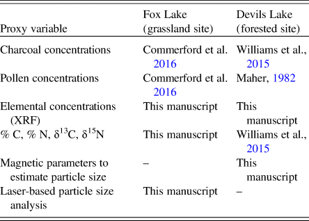
Table 1. Proxy variables for various ecosystem processes, measured on sediment cores from the grassland and forested lakes and presented in this manuscript. Original sources for some of the proxy variables shown in this manuscript are also reported here.

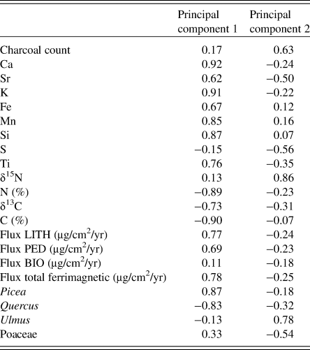
Table 2. The 21 input variables for the principal component analysis of the Devils Lake sediment core and eigenvectors for each variable on the first two principal components.

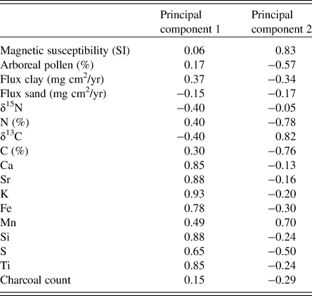
Table 3. The 17 input variables for the principal component analysis of the Fox Lake sediment core and eigenvectors for each variable on the first two principal components.

RESULTS
Sediment sources
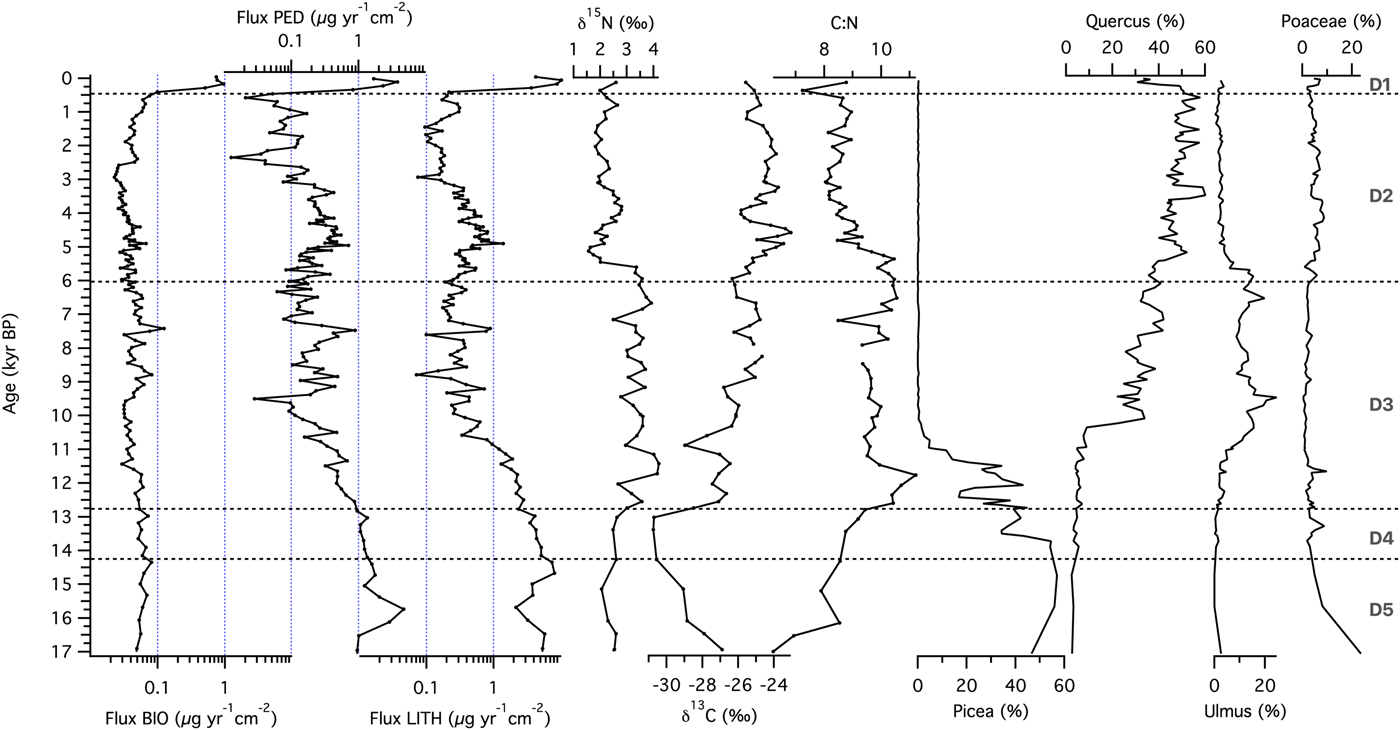
The source material analysis at the forested site (Devils Lake) is based on the magnetic end member fluxes from the unmixing model and the C:N ratio (Fig. 2). The non-biogenic magnetic material input changed over time, with gradual declines in fluxes of both LITH and PED toward present, except for an increase in both components between ~5000 and 3000 cal yr BP. PED fluxes also increased between ~9000 and ~7000 cal yr BP. Magnetofossil flux (BIO) was relatively constant for most of the record, except in the sediments deposited during the past several centuries, when the flux increased by an order of magnitude. The source of the organic matter seems to be aquatic, as evidenced by C:N values that rarely exceeded 10, the ratio found in aquatic microbes and algae.

Figure 2. Source material of sediments at the forested site (Devils Lake, Wisconsin): fluxes of biogenic (BIO), pedogenic (PED), and lithogenic (LITH) ferrimagnetic material calculated from measured magnetic parameters, N and C isotopic composition, and C:N ratio of organic material, and relative abundances of main pollen types. Zones (D1–D5) were based on lithologic transitions in the sediment core identified by Williams et al. (Reference Williams, McLauchlan, Mueller, Mellicant, Myrbo and Lascu2015).
Source material variability during the course of system development at the grassland site (Fox Lake) was evaluated via sediment grain-size analyses and the C:N ratio (Fig. 3). Throughout the record, the flux of silt was dominant, with sand being secondary in importance. Comparatively, only very small amounts of clay were delivered to the sediments for most of the record. Two important shifts should be highlighted: (1) a striking increase in influx of sand-sized particles during the Mid-Holocene around 5500 cal yr BP (zone F3), and (2) an increase in clay and silt influx starting at 1500 cal yr BP (zone F1). The C:N ratio in Fox Lake was almost exclusively >10, indicating that the organic matter was mainly sourced within the catchment. The steady decline of C:N values throughout the Holocene suggests either decreasing terrestrial plant inputs, or an increase in relative abundance of algae and aquatic bacteria (Fig. 3).

Figure 3. Source material of sediments at the grassland site (Fox Lake, Minnesota): fluxes of clay, silt, and sand, N and C isotopic composition, and the C:N ratio of organic material, and relative abundance of arboreal pollen. Zones (F1–F5) were based on magnetic susceptibility transitions in the sediment core identified by Commerford et al. (Reference Commerford, Leys, Mueller and McLauchlan2016).
Sediment geochemistry
To study the sequence of ecosystem processes at each site, we examined temporal patterns of XRF-derived relative elemental abundance. At the forested site Ticlr, Kclr, Siclr, and Caclr were highest in zone D5, then declined during the late glacial, followed by relatively constant values throughout the Holocene, until ~500 cal yr BP (Fig. 4a). Feclr, and Mnclr reached maxima in zone D4, before decreasing throughout the record starting with the Younger Dryas (ca. 12,750 cal yr BP; Hughen et al., Reference Hughen, Southon, Lehman and Overpeck2000). Ticlr, Kclr, Siclr, Caclr, and Feclr reached their Holocene maxima during the first part of the Holocene hypsithermal, between ca. 9500 and 7000 cal yr BP (Dean et al., Reference Dean1997). Sclr experienced a steady increase throughout the record. Element abundances increased in the last few centuries of the record (zone D1). Log ratios of Ti-normalized elemental counts are shown in Figure 4b. Ln(K/Ti) and ln(Si/Ti) demonstrated a pattern of decline toward present, with ln(K/Ti) exhibiting a stronger gradient across the Pleistocene-Holocene transition. Ln(Ca/Ti) values were variable but high in zones D5 and D4, then underwent a sharp transition at ~12,750 cal yr BP, followed by a decrease until 8000 cal yr BP. A local maximum between 8000 and 7000 cal yr BP is followed by relatively constant values for the rest of the record. Ln(Fe/Ti) and ln(Mn/Ti) displayed increasing values until ~9000 cal yr BP, with local maxima in zones D5 (for Mn) and D4 (for Fe and Mn). Both ln(Fe/Ti) and ln(Mn/Ti) displayed pronounced maxima occurred during the Early Holocene (~11,500–9000 cal yr BP). Ln(S/Ti) showed an oscillatory pattern but increased over time toward present.

Figure 4. (color online) (a) Centered-log ratios of selected elements and (b) log ratios of element intensities with respect to the intensity of Ti for sediments from the forested site (Devils Lake, Wisconsin).
Relative elemental abundances in sediments from the grassland site demonstrated a similar pattern to those from the forested site during the Holocene. All seven selected elements demonstrated a long-term decline in abundance from the beginning of the record to present (Fig. 5). This was not a monotonic decline, however. During the early portion of the record (from 9200 to ~8500 cal yr BP, zone F5), when Fox Lake was surrounded by oak woodland, abundances initially increased, with all elements except Sclr exhibiting the highest values in the record at the transition to grassland (ca. 8500 cal yr BP). Other notable peaks occurred in zone F4 (Caclr and Sclr) and around 4000 cal yr BP (Ticlr, Kclr, Siclr, Caclr, Feclr, and Sclr). Log ratios of Ti-normalized counts again revealed different patterns from the absolute counts, with ln(K/Ti) and ln(Si/Ti) declining, ln(Mn/Ti) and ln(Fe/Ti) increasing, and ln(S/Ti) and ln(Ca/Ti) exhibiting variable behavior, with Mid-Holocene maxima.

Figure 5. (color online) (a) Centered-log ratios of selected elements and (b) log ratios of element intensities with respect to the intensity of Ti for sediments from the grassland site (Fox Lake, Minnesota).
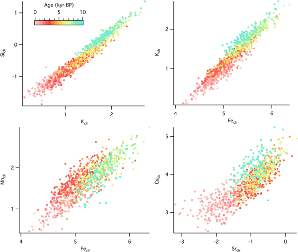
Temporal changes in source material and geochemical structure of sediments can be analyzed with relationships among selected elements. At the forested site, there were positive correlations between Siclr and Kclr (R = 0.91), Kclr and Feclr (R = 0.66), Mnclr and Feclr (R = 0.77), and Caclr and Srclr (R = 0.76), although the correlation strength varied with time (Fig. 6). Slope changes, such as the ones observed in the Kclr-Feclr or Caclr-Srclr biplots, indicate temporal variability in geochemical processes. Relationships among elemental counts at the grassland site showed similar positive correlations (Fig. 7), which were very strong throughout the entire record for Siclr and Kclr (R = 0.97), and Kclr and Feclr (R = 0.96). These two relationships were linear with very little scatter, suggesting similar source material or processes throughout the history of sediment deposition. For Mnclr and Feclr and Caclr and Srclr the correlation was still strong (R = 0.85 and 0.81, respectively), but exhibiting more scatter.
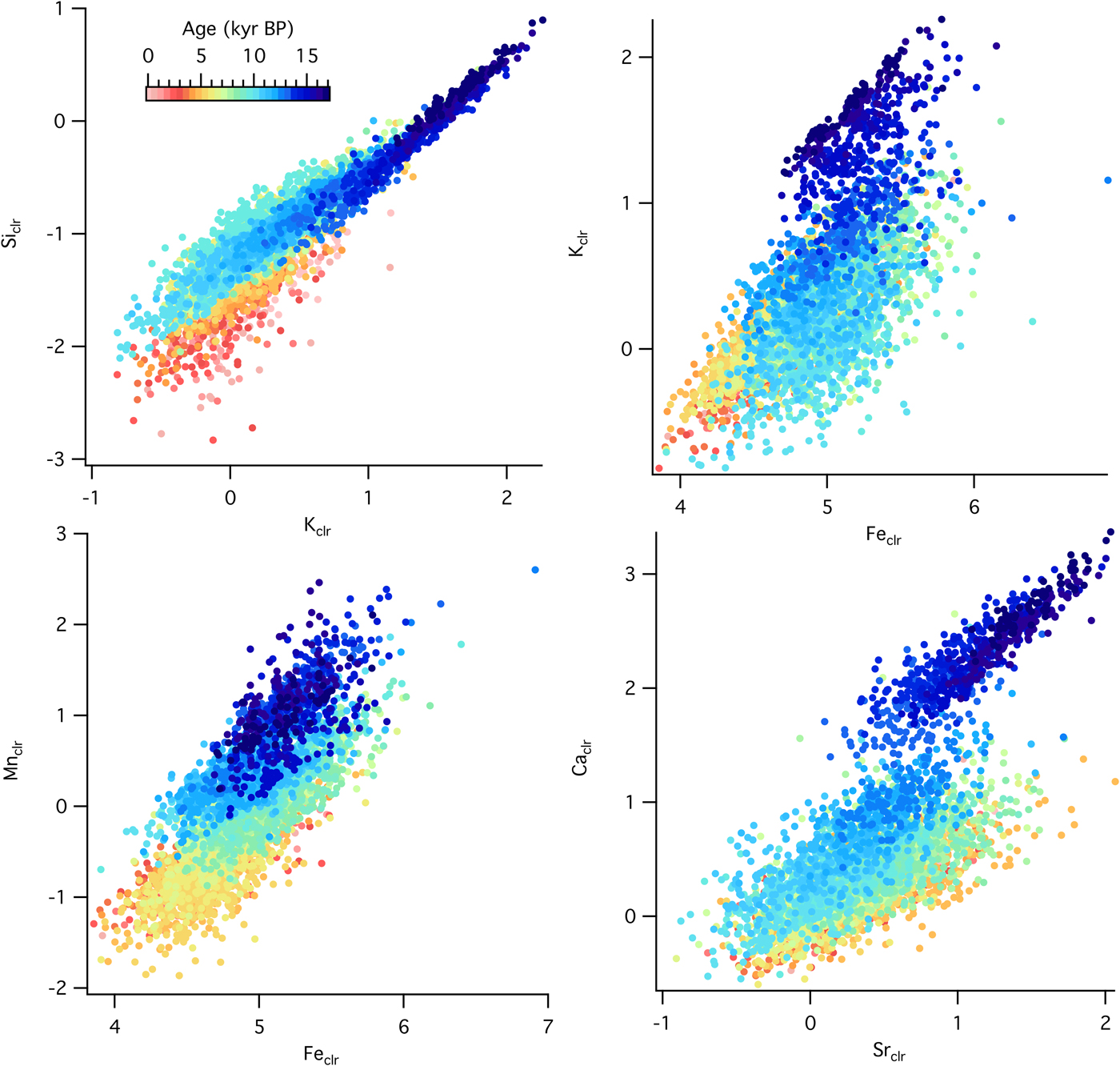
Figure 6. (color online) Cross plots of selected element abundances from the sedimentary sequence at the forested site (Devils Lake, Wisconsin) color coded by time.
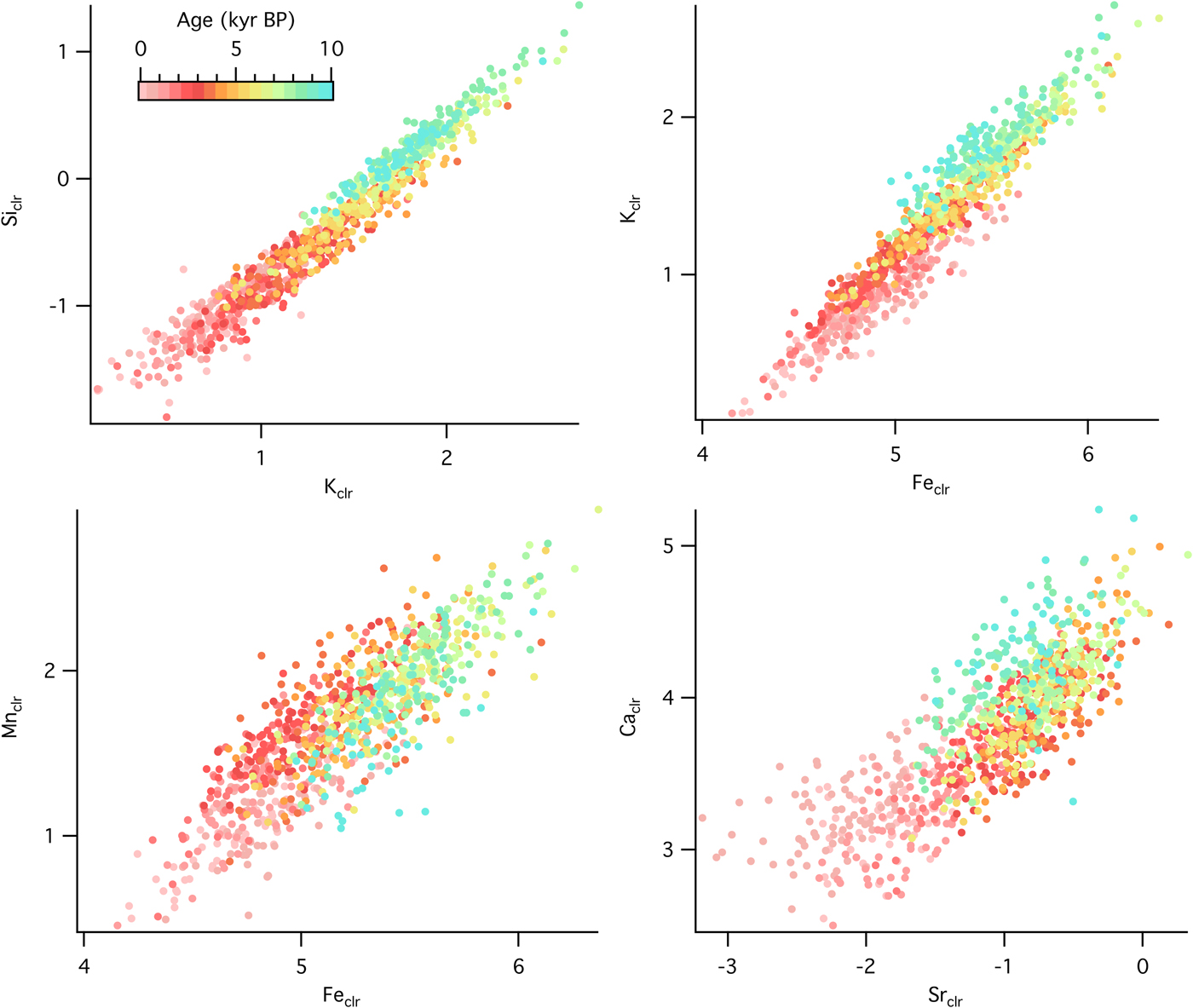
Figure 7. (color online) Cross plots of selected element abundances from the sedimentary sequence at the grassland site (Fox Lake, Minnesota) color coded by time.
Principal component analyses
At the forested site (Fig. 8), the first principal component, explaining 47.7% of the variability in the dataset, followed the stratigraphic trend that showed a major transition from minerogenic to organic-rich sediments after 13,000 cal yr BP (D4-D3 transition). Samples with high values of elemental counts, LITH and PED fluxes, and Picea pollen loaded positively on the first principal component, while samples with high values of δ13C, C and N concentrations, and Quercus pollen loaded negatively on the first principal component. The second principal component, explaining 16.1% of the variability, separated samples high in Ulmus pollen, charcoal, and δ15N from samples high in Poaceae pollen and S concentration.

Figure 8. (color online) Principal components analysis of 21 variables measured on a sediment core spanning the entire sequence of ecosystem development following deglaciation ~17,000 yr from Devils Lake, Wisconsin. (a) Time series of principal components 1 and 2. (b) Score plot of principal components 1 and 2. Circles, data points; diamonds, eigenvectors for each of the variables.
At the grassland site (Fig. 9), the first principal component, explaining 34.8% of the variability in the dataset, displayed periods of little change (e.g., in zone F4), continual decrease (e.g., in zone F3), and continual increase (e.g., in zone F2). Samples with high values of elemental counts loaded positively on the first principal component, and samples with high values of δ15N and sand loaded negatively on the first principal component. The second principal component, explaining 24.3% of the variability, separated samples high in arboreal pollen types and C and N concentrations from samples with high magnetic susceptibility, Mn concentrations, and δ13C values.
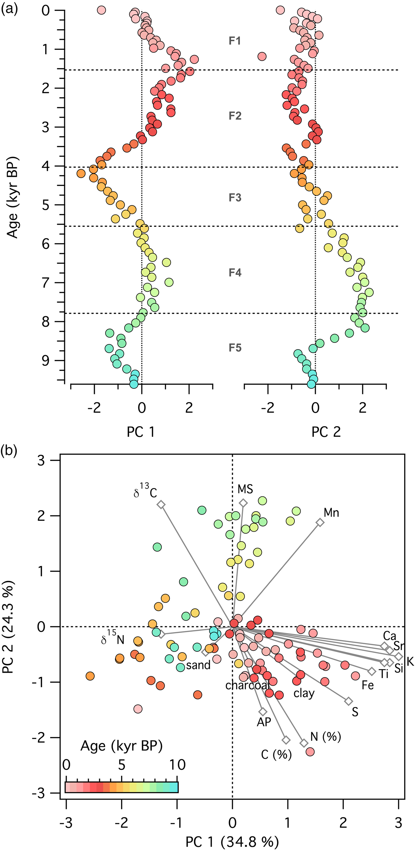
Figure 9. (color online) Principal components analysis of 17 variables measured on a sediment core spanning 9200 yr of ecosystem development following deglaciation from Fox Lake, Minnesota. (a) Time series of principal components 1 and 2. (b) Score plot of principal components 1 and 2. Circles, data points; diamonds, eigenvectors for each of the variables.
DISCUSSION
How did source material change over time?
Source materials at both sites changed as evidenced in the sedimentary sequences. At Fox Lake, progressively lower values of C:N reflect gradually declining terrigenous organic inputs and a shift to a predominance of aquatic algal and bacterial organic matter. A similar pattern was observed at Deming Lake, 425 km to the north of Fox Lake (Fig. 1), with reduced fluxes of both terrestrial organic material and total sediment deposition over the entire 9500-yr sequence (McLauchlan et al., Reference McLauchlan, Lascu, Myrbo and Leavitt2013). The mineral matter flux at Fox Lake increased over time, with the proportion of sand gradually decreasing (except for a transient increase between 5500 and 4000 cal yr BP) in favor of silt and clay, especially for the last 1500 yr.
At Devils Lake, mineral sediment sources shifted from inputs from bedrock sources, as indicated by the pre-Holocene predominance of lithogenic magnetic particles, to catchment soils- and lake-derived material, reflected by increasing amounts of pedogenic and biogenic magnetic particles toward present. A noted exception was the increase of both PED and LITH fluxes during the Mid-Holocene, a warm and dry interval. Several sedimentary records in the region indicate increased eolian influx during this time, such as increased quartz inputs at Elk Lake, Minnesota (Dean, Reference Dean1997). Small inputs of calcareous loess have been noted at Devils Lake during the Mid-Holocene from sources to the west (Grimm et al., Reference Grimm, Maher and Nelson2009). While this would be barely detectable in XRF data as elevated Ca levels, magnetic parameters provide more detail about eolian inputs depending on the size of the wind-blown particles. If they are in the very fine silt size range (2–4 μm), they contribute to the PED component, whereas if they are larger they contribute to LITH fluxes. Abrupt increases in sand influx beginning at 5500 cal yr BP at Fox Lake reflected the proximity to dune fields to the south that mobilized around the same time during increased aridity (Miao et al., Reference Miao, Mason, Swinehart, Loope, Hanson, Goble and Liu2006).
What were the nutrient patterns during Holocene ecosystem development?
While different lengths of time are represented in the records presented here—9200 yr for Fox Lake and 17,000 yr for Devils Lake—the similarity in geochemical patterns indicates that the sequence of processes may be the same across sites although the rate of these processes may vary. Temporal patterns of accumulation of nutrients in the sediments, especially N and base cations, during Holocene ecosystem development indicate striking secular trends. One of the strongest patterns in these records is the slow decline in elemental abundances toward present, reflecting some kind of ontogenetic process or combination of processes. This is especially interesting given the different lithologic settings of these two sites, and the relatively heterogeneous nature of glacial till present on both sites. Lakes in pure bedrock settings, especially basalt and granite with well-established weathering pathways, may demonstrate even clearer signals of geochemical change over time (Sperber et al., Reference Sperber, Chadwick, Casciotti, Peay, Francis, Kim and Vitousek2017; Burghelea et al., Reference Burghelea, Dontsova, Zaharescu, Maier, Huxman, Amistadi, Hunt and Chorover2018)
Similar patterns—declines in concentrations of easily weathered elements such as Ca and Sr—have been documented in late-Pleistocene and Holocene sedimentary records in the Alps (Koinig et al., Reference Koinig, Shotyk, Lotter, Ohlendorf and Sturm2003; Schmidt et al., Reference Schmidt, Kamenik, Tessadri and Koinig2006) and the southern Urals (Maslennikova et al., Reference Maslennikova, Udachin and Aminov2016). Clear signals of N accumulation, as seen in chronosequences (Engstrom et al., Reference Engstrom, Fritz, Almendinger and Juggins2000; Wardle et al., Reference Wardle, Walker and Bardgett2004) and some lake sedimentary sequences (Hu et al., Reference Hu, Finney and Brubaker2001; McLauchlan et al., Reference McLauchlan, Lascu, Myrbo and Leavitt2013), are also seen at Fox Lake in sedimentary δ15N (Fig. 3). An increase in δ15N values at the beginning of the sedimentary record was not as clear at Devils Lake, possibly due to climatic control of N fluxes to the basin during ice sheet retreat and very early landscape evolution (Williams et al., Reference Williams, McLauchlan, Mueller, Mellicant, Myrbo and Lascu2015). It is possible, however, that additional factors confound interpretation of δ15N values as indicating early successional processes.
The relationships between elements show dominantly, but not entirely, abiotic control of elemental ratios. At Fox Lake, Kclr and Caclr both decline from 8000 yr toward present, a time period when grassland vegetation stayed relatively constant (Fig. 5). Si, K, Ti, and Ca abundances in Devils Lake show similar decreasing trends over the first 7000 yr of the record. In the bedrock present at this site, K and Ca are found in extremely low concentrations, as the Baraboo quartzite is both chemically and physically mature (Medaris et al., Reference Medaris, Singer, Dott, Naymark, Johnson and Schott2003). The quartzite and the claystone and siltstone layers interspersed within the quartzite are composed of Si, Ti, Al, and Fe (Medaris et al., Reference Medaris, Singer, Dott, Naymark, Johnson and Schott2003). Early inputs of K and Ca to Devils Lake may have been either from unstable, sparsely vegetated local catchment sources deposited by the retreating glacier, which have subsequently been eroded or chemically weathered, or increased eolian deposition due to drier conditions. Maximum K and Ca abundances in Devils Lake between 9500 and 7000 cal yr BP are more difficult to interpret, as they occur in the middle of zone D3 when vegetation composition is fairly stable. Subsequent stabilization of the catchment has reduced clastic input in the lake and abundances of Ca and K have leveled off after 7000 cal yr BP.
In Devils Lake zone D4, ln(Ca/Ti) increased, in contrast to ln(K/Ti) and ln(Si/Ti), which coincided with peaks in ln(Mn/Ti), ln(Fe/Ti), and ln(S/Ti). These patterns in ratios could be related to a shift to endogenic mineral precipitation, likely due to a change in the redox state of the lake waters in response to climate change during the late glacial interstadial. During this time period, dark, banded microbial sediments were accumulating in deep, stratified lake waters characterized by bottom anoxia (Williams et al., Reference Williams, McLauchlan, Mueller, Mellicant, Myrbo and Lascu2015). Ln(Ca/Ti) decreased suddenly with abrupt cooling at the onset of the Younger Dryas. Throughout the record, the decline in ln(Si/Ti) lagged behind ln(K/Ti), which in turn lagged behind the decline in ln(Ca/Ti), as Ca is more easily mobilized than K during chemical weathering, and Si is the least prone to be dissolved (Nesbitt et al. Reference Nesbitt, Young, McLennan and Keays1996). Ln(Si/Ti) was high at the beginning of the record and decreased afterward, suggesting that initial inputs of lithogenic silica from the catchment during glacial retreat were extremely high. As the catchment stabilized, physical weathering decreased and detrital input decreased. Peaks in ln(Si/Ti) at ~9,500 cal yr BP and to a lesser extent at ~6,500 cal yr BP, may suggest increased contributions from biogenic silica at those times. Despite the appearance of diatoms and corresponding in-lake productivity around 7500 cal yr BP, biogenic silica inputs were not as large as the previous high input of detrital silica.
Fe is correlated to both K and Ti throughout the record at both sites, suggesting that Fe in the lake sediments is mainly detrital. There are time periods characterized by weaker correlation between Fe and K and Fe and Ti, however, especially at the forested site. This points to a more important contribution from authigenic iron-bearing minerals, meaning Fe entered the lake in dissolved form through ground water and precipitated as iron oxides and/or hydroxides. High ln(Fe/Ti) and ln(Mn/Ti), along with abundant vivianite and pyrite in zone D4 (visually identified using petrography), suggest reducing conditions during the late glacial interstadial (Williams et al., Reference Williams, McLauchlan, Mueller, Mellicant, Myrbo and Lascu2015). At the grassland site, the S trend corelates with those of the other elements, suggesting an origin from sulfates in the calcareous tills from the catchment (Gorham et al., Reference Gorham, Dean and Sanger1983). At the forested site, S has an opposite trend to the other elements, suggesting it is associated with organic matter, which increases steadily throughout the record (Williams et al., Reference Williams, McLauchlan, Mueller, Mellicant, Myrbo and Lascu2015).
The Ca-Sr relationship provides additional information about the source material. Concentrations of Ca and Sr in the Baraboo quartzite are extremely low (Medaris et al., Reference Medaris, Singer, Dott, Naymark, Johnson and Schott2003), while the till around Fox Lake is calcareous (Commerford et al., Reference Commerford, Leys, Mueller and McLauchlan2016). Sr often substitutes for Ca in calcium-bearing minerals and is equally mobile during chemical weathering. At Fox Lake, ln(Ca/Sr) is higher during the oak woodland phase prior to 8200 cal yr BP and lower during the grassland phase after 8200 cal yr BP. At Devils Lake, ln(Ca/Sr) is high prior to 12,800 cal yr BP and low and relatively constant from 12,800 cal yr BP to present (Fig. 6). Strong correlation between Ca and Sr indicates a single source for both elements, while a weaker correlation suggests separate provenance, e.g., Ca from an endogenic source and Sr from a lithogenic source.
Climate conditions—hydrologic changes in the catchment, lake level, and evaporation— were considered in other studies to strongly influence elemental concentrations of same seven elements that we studied here (Martin-Puertas et al. Reference Martin-Puertas, Tjallingii, Bloemsma and Brauer2011; Heymann et al., Reference Heymann, Nelle, Dorfler, Zagana, Nowaczyk, Xue and Unkel2013). Lithological composition and mineralogy (quartz silicates, clay silicates, calcite, and coarse particles) have also been considered the dominant factor in determining sedimentary elemental concentrations (Koinig et al., Reference Koinig, Shotyk, Lotter, Ohlendorf and Sturm2003). Declines in elemental concentration could be simply reflecting depletion of mobile elements such as Ca and K from source material in the catchment (Minyuk et al., Reference Minyuk, Borkhodoev and Wennrich2014). In addition to simple first order hydrologic dissolution, there could be a change in the pace of chemical or physical weathering, or changes in transport pathways similar to those observed in Glacier Bay, Alaska during ecosystem development (Milner et al., Reference Milner, Fastie, Chapin, Engstrom and Sharman2007). Recently, a unified “erosion signal” has been identified in alpine lake sediments characterized by changes in elemental concentrations (Arnaud et al., Reference Arnaud, Poulenard, Giguet-Covex, Wilhelm, Revillon, Jenny and Revel2016). In lacustrine settings, Ti is considered a metric of detrital input, so a decline in Ti concentration as observed at both sites in this study likely indicates a gradual decline in detrital input. Finally, there could be further influences through the mechanism by which elements are precipitated in sediments and diagenetic alteration.
Biosphere-lithosphere interactions: did vegetation determine the trajectory of elemental change at each site?
After initial establishment of vegetation at each site, comparisons of vegetation and geochemical change between sites indicate a limited role of vegetation change in influencing geochemical parameters at each site. This generally agrees with other studies that attribute changes in element concentrations in sediment cores to climate-driven changes in weathering and transport processes. An alternative possibility is sediment geochemical change should be attributed to climate-driven vegetation change and subsequent changes in biogeochemical cycling (Martin-Puertas et al., Reference Martin-Puertas, Tjallingii, Bloemsma and Brauer2017). In our study, at both the grassland site and the forested site, the first principal component separated samples with high elemental abundances from those with high organic matter concentration. At the forested site, high Picea pollen loaded positively on the first axis with the elemental counts, and Quercus pollen loaded with organic matter, but this is difficult to interpret purely as a vegetation signal due to a simultaneously warming climate. Thus, there was some correlation of elemental change and forest composition (either hardwood or coniferous forest), but there was also concurrent climate change occurring over the intervals with changes in forest composition.
The other vegetation transitions later in the Holocene at the forested site (involving Ulmus) are only correlated with δ15N, which indicates strong links between vegetation and N cycling throughout the record. Arboreal pollen at Fox Lake and Poaceae (non-arboreal pollen) at Devils Lake loaded in the opposite direction from the N-cycling proxy δ15N at both sites. Early Holocene vegetation reorganization and development of the lake catchment played dominant roles in sediment deposition at Lake Meerfelder Maar, Germany (Martin-Puertas et al., Reference Martin-Puertas, Tjallingii, Bloemsma and Brauer2017). Interactions among vegetation types were important during the transition from glacial to interglacial conditions at the Gerzensee site in Switzerland (Ammann et al., Reference Ammann, van Raden, Schwander, Eicher, Gilli, Bernasconi and van Leeuwen2013), but this may be a due to the relatively large magnitude of vegetation change as indicated in pollen assemblages.
The degree of vegetation change in this study, while notable at each site, is not as large as those demonstrated to causes geochemical changes in other sequences between glacial and interglacial conditions. In particular, differences in primary productivity during stadial-interstadial cycles caused changes in weathering rates at Les Échets, France (Kylander et al., Reference Kylander, Ampel, Wohlfarth and Veres2011), and Lake El'gygytgyn, Russia (Minyuk et al., Reference Minyuk, Borkhodoev and Wennrich2014). The onset of aquatic productivity and organic matter deposition was certainly important at Devils Lake, resulting in anoxic conditions and notable black bands dominated by amorphous aquatic organic material in the sediments (Williams et al., Reference Williams, McLauchlan, Mueller, Mellicant, Myrbo and Lascu2015). While the rate of declining elemental concentrations was altered significantly by this one transition from glacial to interglacial conditions, however, the direction of the trajectory was the same across the transition, indicating a more complex set of processes in addition to plant colonization of a bare landscape. In early succession on recently deglaciated terrain, the timing of establishment of certain plant functional types such as N2 fixers and coniferous trees can have significant effects on accretion of soil C and N, and erosion rates (Crocker and Major, Reference Crocker and Major1955; Fastie, Reference Fastie1995). At Devils Lake, the transition from coniferous to deciduous forest in zone D3 certainly affected fire regime, but not the geochemistry based on the Ti-normalized element concentrations. Finally, geochemical sedimentary records may be able to add detail to the classic view that the relative importance of autogenic and allogenic processes changes over successional time (Matthews, Reference Matthewsp1992).
Another way to assess the role of the terrestrial biosphere is to compare the trajectories between the two sites. The similarities in the sequence of geochemical changes between the forest and the grassland site provide further support for a limited role of vegetation type. Comparisons of absolute rates of change are complicated by different elemental counts between sites, but, for example, declines in ln(K/Ti) and ln(Ca/Ti) seem to be faster at the forested site than at the grassland site. Differences in lithology, topography, and basin size, however, could be more important than vegetation differences between grassland and forest. In particular, Fox Lake is larger and shallower, with calcareous glacial till as parent material and significant agricultural land use in the watershed. Devils Lake is deeper, with non-calcareous glacial till and Precambrian quartzite as parent material and a protected watershed within a state park. As an alternative hypothesis, it is possible that climate change was directly influencing geochemistry through catchment weathering and hydrologic transport of material into the lake basin. Further estimates of weathering rates, catchment destabilization due to aridity, or hydrologic fluxes over Holocene timescales would help test these hypotheses.
CONCLUSIONS
To assess rates, patterns, and mechanisms of ecosystem development after glacial retreat, we compared two sedimentary sequences in the upper Midwestern United States, one from a grassland site and a forested site. We found that source material changed over the Holocene sedimentary sequences. We also found that the patterns of nutrients, especially limiting nutrients such as N, K, Ca, and Mg, changed over the Holocene sedimentary sequences. It seems that once vegetation was established, there was minimal influence of vegetation composition on inorganic sediment properties thereafter. At the forested site, transitions among vegetation from Picea to Pinus to deciduous hardwood led to changes in fire regime and nutrient cycling but not inorganic element abundances. At the grassland site, the transition from oak forest to grassland affected primarily delivery of organic material to the catchment. There is future potential to interpret sedimentary elemental concentrations in light of ecological processes. Two aspects are likely to make these successful: (1) comparing several sites with different vegetation histories, and (2) measuring many proxies to help provide independent estimates of multiple processes influencing sediment records.
ACKNOWLEDGMENTS
We thank J. Mueller, S. McConaghy, J. Commerford, A. Myrbo, K. Brady, A. Lingwall, T. Ocheltree, R. Paulman, and R. Keen for field and laboratory assistance. J. L. Morris provided helpful discussion about the Fox Lake XRF data. We thank Catherine Yansa and an anonymous reviewer for comments that greatly improved the manuscript. Financial support was provided by National Science Foundation BCS-0955225 to K.M. and a Kansas State University College of Arts and Sciences Undergraduate Scholarship to R.S. Support for I.L. was provided through ERC grant 320750 under the European Union's Seventh Framework Programme (FP/2007-2013). KM managed the project and led manuscript preparation. IL led data analysis and figure conception. IL, EM, and KM led data interpretation. All authors generated primary data from Fox Lake and/or Devils Lake sediment cores, and all authors discussed results and contributed to manuscript preparation.