


INTRODUCTION
Identifying the locations of paleo–ice streams and characterizing their evolution is essential for understanding ice-sheet deglaciation, as ice streams impact the rate of ice discharge (Bamber et al., Reference Bamber, Vaughan and Joughin2000; Livingstone et al., Reference Livingstone, Ó Cofaigh, Stokes, Hillenbrand, Vieli and Jamieson2012). The Oneida Ice Stream, located between modern Lake Ontario and Oneida Lake, was a major ice stream of the Laurentide Ice Sheet (LIS). It was identified by light detection and ranging (LIDAR) data and digital elevation models that revealed drumlins and megascale glacial lineations (MSGLs) west of the Oneida basin (Briner, Reference Briner2007; Murari et al., Reference Murari, Domack and Owen2016; Sookhan et al., Reference Sookhan, Eyles and Putkinen2018). The cause of this change in bedform morphology cannot be fully assessed by LIDAR data, as glacial bedforms in the Oneida basin are largely buried by proglacial lake deposits (Briner, Reference Briner2007; Sookhan et al., Reference Sookhan, Eyles and Putkinen2018). Therefore, subsurface investigations of Oneida Lake are required to better understand the retreat, extent, and ice flow velocities of a critical section of the Oneida Ice Stream. Determining depth to the preglacial surface of the Oneida basin is particularly important, as paleo–ice flow velocities of the Oneida Ice Stream are interpreted to be highest west of the lake (Briner, Reference Briner2007; Hess and Briner, Reference Hess and Briner2009) and possibly influenced by the basin (see Supplementary Fig. S1).
Ice discharge rates, surges in ice streams, and catastrophic releases of glacial meltwater from proglacial lakes can have profound effects on Northern Hemisphere climate (Broecker et al., Reference Broecker, Kennett, Flower, Teller, Trumbore, Bonani and Wolfi1989; MacAyeal, Reference MacAyeal1993; Broecker, Reference Broecker1994; McCabe and Clark, Reference McCabe and Clark1998). The Younger Dryas has been studied intensively for these reasons, as it is thought that a large release of meltwater triggered the event (Broecker et al., Reference Broecker, Kennett, Flower, Teller, Trumbore, Bonani and Wolfi1989; Clark et al., Reference Clark, Marshall, Clarke, Hostetler, Licciardi and Teller2001; Leydet et al., Reference Leydet, Carlson, Teller, Breckenridge, Barth, Ullman, Sinclair, Milne, Cuzzone and Caffee2018). Multiple shorter-lived abrupt cold stadials at the end-Pleistocene are identified in climate records, including the Older Dryas stadial (ca. 14.3–14 cal ka BP) and the Intra-Allerød period (ca. 13.35–13.1 cal ka BP). These cold stadials have received much less attention and may have been triggered by proglacial lake meltwater releases as well (Rasmussen et al., Reference Rasmussen, Andersen, Svensson, Steffensen, Vinther, Clausen and Siggaard-Andersen2006, Reference Rasmussen, Bigler, Blockley, Blunier, Buchardt, Clausen and Cvijanovic2014; Ridge et al., Reference Ridge, Balco, Bayless, Beck, Carter, Dean, Voytek and Wei2012). However, the proglacial lake deposits in Oneida Lake likely contain a paleoclimate record spanning all of these cold stadials that until now has been overlooked and that can provide constraints on Ontario Lobe fluctuations (Fig. 1). Comparing records of Ontario Lobe meltwater production with Greenland Ice Sheet records can help better constrain the connection between the LIS deglaciation and North Atlantic climate, as was completed for LIS lobes east of the Ontario Lobe (Ridge et al., Reference Ridge, Balco, Bayless, Beck, Carter, Dean, Voytek and Wei2012).

Figure 1. Digital elevation model (acquired from the USGS) of the study region with a box indicating the location of Oneida Lake and the location of important Laurentide Ice Sheet (LIS) ice margins and the Glacial Lake Iroquois shoreline. The northern shoreline of the lake in many locations was the LIS. Tick marks on the ice margins indicate glacial ice; the Mohawk Lobe was located well to the east of the study area, whereas the Oneida Lobe occupied the region of modern-day Oneida Lake (Ridge, Reference Ridge, Ehlers and Gibbard2004; Bird and Kozlowski, Reference Bird and Kozlowski2016; Franzi et al., Reference Franzi, Ridge, Pair, Desimone, Rayburn and Barclay2016; Dalton et al., Reference Dalton, Margold, Stokes, Tarasov, Dyke, Adams and Allard2020).
This paper presents multichannel seismic reflection (MCS) data collected within Oneida Lake in 2019. In addition, high-resolution single-channel Compressed High Intensity Radiated Pulse (CHIRP) data collected before the MCS data are also presented (Zaremba and Scholz, Reference Zaremba and Scholz2019). The entire Quaternary section of the lake is imaged, including previously unknown glacial bedforms, the glacial sediment–bedrock interface (~90 m from the modern lake surface), and the complete proglacial lake sedimentary section, which leads to a better understanding of the evolution of the Oneida Ice Stream and the extent of proglacial lake deposits within the basin.
REGIONAL SETTING
Regional deglaciation
The Oneida Lobe is a sublobe of the larger Ontario Lobe of the Laurentide Ice Sheet and occupied the Mohawk Valley and the Oneida basin until ca. 14.8 cal ka BP (Ridge, Reference Ridge, Ehlers and Gibbard2004; Franzi et al., Reference Franzi, Ridge, Pair, Desimone, Rayburn and Barclay2016; Fig. 1). The timing of retreat of the Oneida Lobe has been interpreted by mapping the location of recessional moraines, with temporal constraints extrapolated from a radiocarbon-dated varve chronology (Ridge, Reference Ridge, Ehlers and Gibbard2004; Ridge et al., Reference Ridge, Balco, Bayless, Beck, Carter, Dean, Voytek and Wei2012; Franzi et al., Reference Franzi, Ridge, Pair, Desimone, Rayburn and Barclay2016). The varve chronology (North American Varve Chronology Project), was developed primarily from outcrops and cores from the Champlain and Hudson Valleys east of the Oneida basin (Ridge, Reference Ridge, Ehlers and Gibbard2004; Ridge et al., Reference Ridge, Balco, Bayless, Beck, Carter, Dean, Voytek and Wei2012; Franzi et al., Reference Franzi, Ridge, Pair, Desimone, Rayburn and Barclay2016; Fig. 1). A readvance of the LIS at the end of the Erie Interstadial ca. 17 cal ka BP is one of the most important events in the region, as it is responsible for deposition of the Valley Heads Moraine, a prominent glacial feature in the region (Ridge, Reference Ridge1997). As the Oneida Lobe readvanced eastward, the Mohawk Lobe simultaneously readvanced westward, blocking drainage of meltwater via the Mohawk Valley and redirecting meltwater south and west to the Susquehanna River (Franzi et al., Reference Franzi, Ridge, Pair, Desimone, Rayburn and Barclay2016; Fig. 1). These ice lobes blocked meltwater drainage outlets, creating deep, expanding proglacial lakes (Ridge et al.,Reference Ridge, Franzi and Muller1991; Franzi et al., Reference Franzi, Ridge, Pair, Desimone, Rayburn and Barclay2016). Even with the formation of these large proglacial lakes, the Oneida Lobe continued to advance eastward, while the westward-flowing Mohawk Lobe retreated to the east (Franzi et al., Reference Franzi, Ridge, Pair, Desimone, Rayburn and Barclay2016). It is postulated that the Mohawk Lobe retreated as a result of frontal calving into the deep proglacial lakes, whereas the Oneida Lobe was stabilized by the narrow valley it occupied (Sookhan et al., Reference Sookhan, Eyles and Putkinen2018). Eventually, the Mohawk Lobe retreated far enough east to reroute drainage of glacial meltwater back through the Mohawk Valley and into the Hudson Valley. The Oneida Lobe readvanced and retreated multiple times until ca. 14.5 cal ka BP, when the Oneida basin was inundated, forming Glacial Lake Iroquois (Franzi et al., Reference Franzi, Ridge, Pair, Desimone, Rayburn and Barclay2016).
The proglacial deposits from Glacial Lake Iroquois should provide a detailed paleoclimate record and insights into meltwater processes. Glacial Lake Iroquois was an extensive proglacial lake covering modern Lake Ontario and Oneida Lake. This proglacial lake drained via the Mohawk Valley into the Hudson River Valley and into the North Atlantic Ocean (Fig. 1). The uncovering of a topographic low at Covey Hill ca. 13.2 cal ka BP allowed for catastrophic northward drainage of Glacial Lake Iroquois into the Champlain Lowlands and into the North Atlantic Ocean (Donnelly et al., Reference Donnelly, Driscoll, Uchupi, Keigwin, Schwab, Thieler and Swift2005; Rayburn et al., Reference Rayburn, Knuepfer and Franzi2005, Reference Rayburn, Franzi and Knuepfer2007). The formation of Glacial Lake Iroquois, deposition of proglacial lake deposits, and alterations in drainage occurred over a time period that included the Older Dryas (ca. 14.3–14.0 cal ka BP), intra-Allerød cold period (ca. 13.35–13.1 cal ka BP), and Younger Dryas (ca. 12.9–11.8k cal ka BP) events, all identified as abrupt cold periods in the North Atlantic region (Stuiver et al., Reference Stuiver, Grootes and Braziunas1995; Rasmussen et al., Reference Rasmussen, Andersen, Svensson, Steffensen, Vinther, Clausen and Siggaard-Andersen2006, Reference Rasmussen, Bigler, Blockley, Blunier, Buchardt, Clausen and Cvijanovic2014; Ridge et al., Reference Ridge, Balco, Bayless, Beck, Carter, Dean, Voytek and Wei2012).
New York Drumlin Field and Valley Heads Moraine
The Valley Heads advance was important in the routing of glacial meltwater. The Valley Heads Moraine marks the southernmost limit of glacially streamlined bedforms indicative of ice-streaming processes (Sookhan et al., Reference Sookhan, Eyles and Putkinen2018). Sookhan et al. (Reference Sookhan, Eyles and Putkinen2018) postulated that ice streaming did not occur within the region until after deposition of the Valley Heads Moraine and that formation of large proglacial lakes could have caused frontal calving, thereby increasing ice flow velocities and encouraging ice stream formation (Sookhan et al., Reference Sookhan, Eyles and Putkinen2018). Analysis of the orientation and length-to-width ratios of drumlins and MSGLs within the New York Drumlin Field has helped identify the location of multiple former ice streams or areas of increased ice flow that occurred during retreat of the Laurentide Ice Sheet (Briner, Reference Briner2007; Hess and Briner, Reference Hess and Briner2009; Menzies et al., Reference Menzies, Hess, Rice, Wagner and Ravier2016; Sookhan et al., Reference Sookhan, Eyles and Putkinen2018; see Supplementary Fig. S1). The location of the Oneida Ice Stream has been identified to the west and north of the Oneida basin between Lake Ontario and Oneida Lake (Briner, Reference Briner2007; Hess and Briner, Reference Hess and Briner2009; Margold et al., Reference Margold, Stokes and Clark2015a, Reference Margold, Stokes, Clark and Kleman2015b; Sookhan et al., Reference Sookhan, Eyles and Putkinen2018; Fig. 1). Bedform elongation ratios and therefore paleo-ice velocities are highest on the western shoreline of Oneida Lake (Briner, Reference Briner2007; Hess and Briner, Reference Hess and Briner2009). However, such studies are limited to characterizing the surficial expression of glacial bedforms, some of which are buried by proglacial lake deposits. With retreat of the Oneida Lobe, Glacial Lake Iroquois inundated the basin and buried many subglacial bedforms with proglacial lake deposits (Sookhan et al., Reference Sookhan, Eyles and Putkinen2018; Zaremba and Scholz, Reference Zaremba and Scholz2019).
METHODS
Seismic reflection data acquisition
In July of 2019, ~217 km of 2D MCS data were collected along 27 profiles. We used a 120 channel Seamux solid-towed array marine streamer with a 3.125 m group interval and a maximum offset of ~400 m. A 4 × 10 in3 Bolt 2800 LLX airgun array was used as the seismic source and was towed at ~1 m depth to allow for venting of seismic-source air bubbles. Airguns were fired every 6.25 m distance using two high-resolution (Trimble) GPS receivers for navigation. This geometry provided 30-fold seismic coverage with a common midpoint (CMP) interval of 1.56 m. Record length was 2 s, and the sample rate was 0.25 ms.
MCS data processing
The following processing steps were applied to the data set using SeisSpace/ProMAX software. Data were initially reviewed in shot mode, and noisy traces were edited. Geometry was applied using source and receiver offsets with group and shot intervals, and data were sorted into the CMP domains. Stacking velocities were picked using a combination of velocity semblance plots and constant velocity stacks applied to CMP supergathers. For the constant velocity stacks, supergathers were constructed from 51 CMPs and analyzed in increments of 100 CMPs. Once time–velocity pairs were selected, normal moveout was applied, and the data were stacked. Nested Ormsby band-pass filters of 110-135-1500-1700 Hz and 40-70-1100-1300 Hz were applied to the stacked data sets. Ormsby filter frequencies were picked by executing a careful parameter test whereby frequencies were altered incrementally until the ideal filter was produced. A post-stack F-K filter was applied to remove steeply dipping noise, and a careful comparison of F-K filtered profiles and raw profiles was conducted. A post-stack Kirchhoff time migration with a 200 ms bottom taper was applied using the root mean square stacking velocities picked for each seismic profile. The MCS data provide vastly improved signal-to-noise ratio of deeper strata and enhance imaging of deep structures compared with the high-resolution single-channel (Compressed High Intensity Radiated Pulse) CHIRP data. Multichannel seismic data included in this paper are available for download at the Marine Geosciences Data System (https://www.marine-geo.org/tools/search/entry.php?id=Oneida_MCS_SU).
Interactive seismic reflection data interpretation
Seismic profiles were loaded into Landmark DecisionSpace™ software for interactive interpretation. Seismic horizons were interpreted and gridded for the generation of sediment thickness and depth-to-horizon maps. All gridding and contouring was completed in the two-way travel time domain. The Reflection 1 surface was gridded using DecisionSpace's refinement gridding algorithm, similar to a least-squares gridding approach. Refinement gridding begins with a coarse grid and refines the surface to create a series of finer grids, allowing for creation of intermediate grid values based on the original data.
The till isopach map (Fig. 2B) was gridded using DecisionSpace's isopach algorithm. The isopach algorithm also uses a least-squares algorithm but sets a grid minimum value to 0 ms and has no lower bounds to the z-value. For the till thickness computations, we gridded areas with higher seismic line density using a smaller search radius (400 m) and a smaller grid size (250 m), and areas elsewhere in the lake were gridded using search radius of 500 m and a grid size of 400 m.

Figure 2. (A) Depth to top of till (in two-way travel time [twtt]) produced from multichannel seismic reflection data (black lines) and high-resolution Compressed High Intensity Radiated Pulse (CHIRP) data (purple lines) (Zaremba and Scholz, Reference Zaremba and Scholz2019). The basin in the east is indicated in dark blue, while the Paleozoic high is indicated by orange and red in the central section of the lake. MCS, multichannel seismic reflection; twtt, two-way travel time. (B) Till isopach (in twtt) and surficial geology of the area adapted from Muller and Cadwell (Reference Muller and Cadwell1986). The map produced by Muller and Cadwell is the result of combining multiple surficial geology quadrangles from the USGS and other sources. Similar to A, dark blue indicates thick till (~45 ms twtt), red indicates thin till. The black outlines indicate the location of polygons where search radius and cell size were altered based on density of seismic lines. Areas inside the polygons represent higher line density and therefore a smaller search radius and cell size. Cell size was 250 m outside the polygons and 100 m inside the polygons. Search radius was 500 m outside the polygons and 400 m inside the polygons. Note that till is primarily thicker in the north basin and thin over the Paleozoic high and shallow south basin, likely a result of englacial water distribution and ice flow velocities.
Velocity analysis from refractions
Refraction arrivals from high-velocity strata are commonly observed on shot gathers across the entire study area (Fig. 3). Velocities independent of those from semblance analyses or constant velocity stacks can be estimated based on refraction arrival times.

Figure 3. (A and B) Grooves incised into the Paleozoic high from possible ice streaming. Grooves range in height from 3 to 6 m with an apparent horizontal spacing of ~180 m. (C) Refraction data from a single shot from line MCS-08 indicate the arrival of a refracted wave traveling at ~4500 m/s, indicating lithified material interpreted as top of Paleozoic strata. MCS, multichannel seismic reflection; twtt, two-way travel time.
RESULTS
Data processing
Data processing resulted in eight variations or eight processed data sets for every line. These data sets included one of the following or a combination of the following data-processing techniques for each line: a Kirchhoff time migration, post-stack F-K filter and band-pass filters as described in “Methods.” Kirchhoff time migrations succeeded in collapsing point reflections, which aided in discerning steeply dipping ridges from point reflections (Fig. 3). The F-K filter removed a significant amount of steeply dipping noise and the band-pass filter aided in interpreting important horizons. The seismic profiles presented in this paper were processed with a F-K filter and Kirchhoff migration.
All stacking velocities were overlaid in color on top of the seismic reflection profiles to aid in geologic interpretation. Stacking velocities of ~1480 m/s to 1600 m/s are observed in the uppermost sections (e.g., Figs. 4B and 5B) with increases to 1700–2200 m/s with the first significant seismic facies change.

Figure 4. (A) Glacially streamlined bedforms interpreted as drumlins (Group 2). The seismic profile crosses drumlins oblique to ice flow direction. Note the rise in the Paleozoic bedrock beneath the drumlins, suggesting the preglacial topography had an influence on drumlin formation. (B) Stacking velocities overlain on profile. Velocities of proglacial deposits (U2A) are 1500–1600 m/s, whereas till (U1) velocities are 1700–2000 m/s. MCS, multichannel seismic reflection; twtt, two-way travel time.

Figure 5. Three seismic profiles that image multiple sharp-crested symmetrical ridges interpreted as De Geer moraines (Group 3). These sharp-crested ridges are similar in dimension to many documented De Geer moraines, with relief of 3–12 m, and spacing as tight as 70 m. (A) De Geer moraines are well imaged, despite the effects of a mass transport deposit in the proglacial, point reflections, and attenuation of the signal from biogenic gas above the De Geer moraines. (B) E-W profile includes the uninterpreted and interpreted profiles and a stacking velocity overlay. (C) N-S seismic profile images the sharp-crested symmetrical ridges (Group 3). MCS, multichannel seismic reflection; root mean square, RMS; twtt, two-way travel time.
Descriptions and interpretations
The MCS data indicate that Quaternary sediments of Oneida Lake occupy two subbasins that trend NW to SE (Fig. 2A). The northern subbasin reaches a maximum depth of ~120 ms two-way travel time (twtt) (~90 m) below the modern lake surface, with a maximum sediment thickness of ~105 ms twtt (~78 m). The southern subbasin extends to a maximum depth of ~45 ms twtt (~34 m) from the modern lake surface, with a maximum thickness of ~30 ms twtt (~23 m) (Fig. 2A). The seismic facies infilling these basins vary from transparent to highly continuous, low-amplitude reflections that drape the underlying basal reflection.
Three stratigraphic units have been identified within the basins based on external geometry, internal reflections, reflection amplitude, and refraction and reflection velocities (Figs. 6 and 7). In addition, high-resolution CHIRP seismic data were used to aid in interpreting the upper stratigraphic units and in delineating the orientation of various stratigraphic units and glacial bedforms (Zaremba and Scholz, Reference Zaremba and Scholz2019). Unit 1 contains multiple distinct glacial bedforms identified based on the geometry of the upper bounding reflection. High-resolution CHIRP data image three subunits within Unit 2, but those are not discriminated in the MCS data, given its lower frequency range.
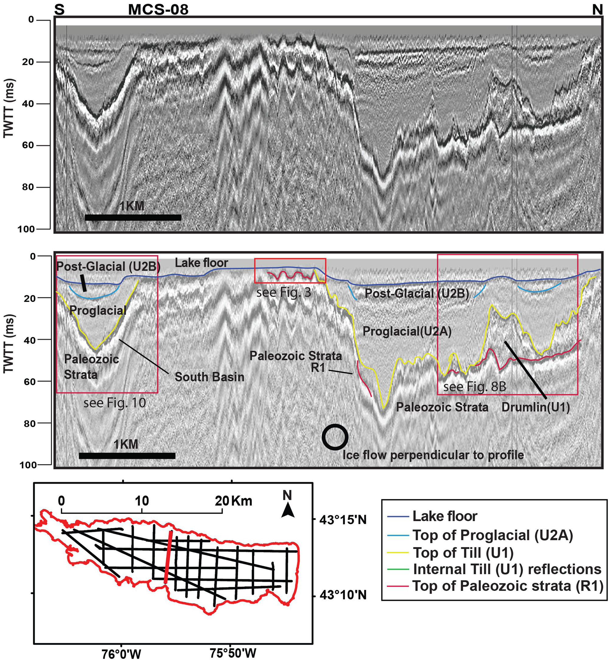
Figure 6. Uninterpreted and interpreted profiles of MCS-08; inset map indicates location of the seismic line. N-S profile crosses the entire lake and shows overall basin geometry, including the two subbasins and the Paleozoic high. For a more detailed view of the grooves incised into the Paleozoic strata see Fig. 3B; for the drumlin in the right-hand corner of the profile, see Fig. 8B; for the thin till in the south basin, see Fig. 10. MCS, multichannel seismic reflection; twtt, two-way travel time.

Figure 7. Seismic facies observed in Oneida Lake, and corollary interpretations.

Figure 8. (A) E-W uninterpreted and interpreted profiles from northern subbasin. Multiple glacially streamlined bedforms interpreted as drumlins. Seismic profiles cross the drumlin oblique to ice flow direction and contain multiple internal reflections, suggesting the drumlin was of depositional origin. Approximate drumlin location is delineated by a transparent yellow shape. (B) N-S MCS profile 08 images the same drumlin as in 8A, however, perpendicular to ice flow in B. Approximate drumlin location is delineated by a transparent yellow shape. (C) Compressed High Intensity Radiated Pulse (CHIRP) seismic profile over same area constrains the orientation of glacial bedforms in the data set. Acoustic basement in CHIRP profiles is the top of the till. MCS, multichannel seismic reflection; twtt, two-way travel time.
Description, Reflection 1
Reflection 1 is the highest amplitude reflection imaged within the data set (Figs. 3, 6 and 7). It is easily identified and well imaged in the center of the lake, where it occurs as shallow as 7 ms twtt (~6 m) below the lake surface. Reflection 1 is imaged ~120 ms twtt (90 m) below the modern lake surface in the eastern section of the lake; however, the reflector is likely deeper farther to the east, where seismic amplitudes are attenuated (Fig. 2B). The reflecting surface varies from flat to undulatory with vertical amplitudes of up to 6 m over a horizontal distance of 90 m. This undulatory topography occurs over the center of the lake (Figs. 3 and 6). Refraction arrivals indicate a velocity of approximately 4 km/s for Reflection 1 (Fig. 3C).
Interpretation, Reflection 1 (R1): top of Paleozoic strata
Refraction velocities of approximately 4 km/s originating from the approximate depth of Reflection 1 suggest the deeper strata consist of old, dense, well-lithified material, and not poorly consolidated or unlithified Quaternary deposits (Pinson et al., Reference Pinson, Vardy, Dix, Henstock, Bull and Maclachlan2013; Stumpf and Ismail, Reference Stumpf and Ismail2013; Fig. 3C). Studies of Appalachian basin Paleozoic strata suggest velocities similar to those provided by the refraction velocities derived from this study (Engelder, Reference Engelder1979; Zhu, Reference Zhu2013). Accordingly we interpret Reflection 1 as the top of the Paleozoic strata, and most likely the Herkimer Sandstone of the Clinton Group (Rickard and Fisher, Reference Rickard and Fisher1970; see Supplementary Fig. S2). The ridge and swale relief of the inferred Paleozoic strata is imaged in multiple seismic lines that extend N-S across the basin, perpendicular to ice flow (Figs. 5 and 6). We interpret the ridge and swale topography as megagrooves or grooves incised by ice streaming processes, similar to those observed in other regions covered by ice sheets in the late Pleistocene (Bradwell et al., Reference Bradwell, Stoker and Krabbendam2008; Krabbendam et al., Reference Krabbendam, Eyles, Putkinen, Bradwell and Arbelaez-Moreno2016; Bukhari et al., Reference Bukhari, Sookhan, Eyles, Shi, Mulligan and Paulen2020). The 90 m wavelengths between ridges and 6 m amplitudes are comparable to the dimensions of megagrooves observed in other studies (Bradwell et al., Reference Bradwell, Stoker and Krabbendam2008; Krabbendam et al., Reference Krabbendam, Eyles, Putkinen, Bradwell and Arbelaez-Moreno2016; Bukhari et al., Reference Bukhari, Sookhan, Eyles, Shi, Mulligan and Paulen2020). Outcrops of the Paleozoic strata in the surrounding area indicate undeformed strata with low dips, suggesting the ridge and swale relief is not a result of deeper Paleozoic structures.
Description, Unit 1 (U1)
Unit 1 is highly variable in thickness, ranging from 3 to 45 ms twtt (3–45 m) thick at a depth of 7–120 ms twtt (6–90 m) below the modern lake surface (Fig. 2). The top bounding surface of Unit 1 is highly variable, flat in places or otherwise hummocky and or rugose (Figs. 4, 6, 8 and 9). Unit 1 contains multiple internal point reflections or diffractions as well as discontinuous internal stratal reflections, but the unit is primarily transparent or internally homogenous. In the western section of the lake, it outcrops above the lake surface, forming several islands. The unit is imaged throughout most of the lake but is mostly absent in the south basin.

Figure 9. (A) N-S seismic profile images (uninterpreted and interpreted) of the deep basin in the eastern section of the lake, as well as the thick sheet of till interpreted as a moraine (Group 1). (B) E-W profile images thick sheet of till interpreted as a moraine (Group 1); it intersects profile in A, as indicated by the red vertical line. The upper bounding surface of the till (yellow reflection) is hummocky or contains small sharp-crested symmetrical ridges, possibly De Geer moraines. MCS, multichannel seismic reflection; twtt, two-way travel time.
Interpretation, Unit 1 (U1): Till
Unit 1 is interpreted as till deposited by the ice sheet. Three primary glacial landforms have been identified based on the geometry of the upper bounding reflection (Figs. 2A, 4, 5 and 7–9). Especially evident are bedforms and glacial features interpreted as the result of deformation and deposition during ice streaming and grounding-line retreat of the ice sheet. The identified features suggest ice streaming processes were operative in the basin, as they were to the west of the modern lake (Hess and Briner, Reference Hess and Briner2009).
The till section in the southern section of the lake is remarkably thin compared with the north basin; it is possible that meltwater may have eroded and removed till from this area (Fig. 10). No truncation of till surfaces is observed in the north basin. The depth to the top of the Paleozoic strata is generally shallower in the southern section of Oneida Lake and may in part be responsible for a thin or absent till section there. The till thickness in the easternmost part of Oneida Lake is equivocal, on account of biogenic gas in the near surface (Fig. 2A). Unit 1 consists of till and, based on the thickness of the unit and geometry of the upper bounding surface, can be separated into three distinct glacial landform groups described in the following sections.

Figure 10. N-S seismic profile across the south basin. The till (U1) is thin to absent in the south basin, whereas proglacial (U2A) and postglacial (U2B) units are well imaged. MCS, multichannel seismic reflection; twtt, two-way travel time.
Description, Glacial Landform Group 1
The lower bounding surface of Glacial Landform Group 1 is Reflection 1, interpreted to be Paleozoic bedrock. The upper bounding surface ranges from flat to hummocky to a low-amplitude, symmetrical, ridge and swale topography, 4–10 ms twtt (~3–7 m) in height. Moderate-amplitude, dipping internal reflections are present but rare in Group 1. Group 1 is highly variable in thickness, reaching a maximum of 35 ms twtt (~35 m) (Fig. 2A) in a few locations (Fig. 9). Group 1 thins in the deepest section of the E-W oriented axis of the basin (Fig. 1) and is observed primarily in the central and eastern sections of the lake. Group 1 is distinctive in that it is the most continuous, relatively thick sheet of till imaged in the basin. In other locations, the till is thin to absent or highly variable in thickness over short distances.
Interpretation, Glacial Landform Group 1: reworked moraine?
Group 1 is a thick section of till interpreted to be accumulation of debris that was advected from the Oneida Ice Stream and deposited near the terminus of the ice sheet. The thick section of till thins with depth, possibly as a result of erosion from fast-flowing meltwater after initial deposition and retreat of the ice sheet (Fig. 9A). The undulating upper bounding layer of Group 1 suggests the till was slightly modified during final retreat of the ice sheet as well (Fig. 9). We cannot be entirely sure of the original dimensions of Group 1. However, a thick succession of till that extends north to south or approximately perpendicular to the direction of ice flow could be interpreted to be the remnants of a moraine of some type. Accordingly, we tentatively interpret Group 1 to be a moraine reworked from meltwater processes.
Description, Glacial Landform Group 2
Glacial Landform Group 2 is imaged within the north-central and northwestern sections of the lake and reaches a maximum thickness of 45 ms twtt (~45 m) (Fig. 2B). Group 2's lower bounding surface is Reflection 1 (Figs. 4 and 8). In a few instances, Group 2 outcrops above the lake floor and lake surface, forming islands in the NW section of the lake (Fig. 4). Group 2 is highly variable in relief, with multiple steep-sided oblong or oval-shaped hills with dips of ~6°–8° to the NE or SW. The height of these hills varies from 18 to 28 m. The short axis of each individual hill is 200–500 m in length, and the long axis is 700–2700 m in length, with a NW to SE orientation. Furthermore, stacked internal dipping reflections are commonly imaged below the bounding reflector of these hills (Fig. 8A), while others are transparent (Fig. 8).
Interpretation, Glacial Landform Group 2: drumlin field
Group 2 is interpreted as a drumlin field based on the on the size, shape, orientation, and elongation ratio of the glacial bedforms (Figs. 4, 8, and 11). Elongation ratios (length:width) are used to define the type of glacially streamlined bedforms, and drumlins are defined as features with elongation ratios below 10:1. Megascale glacial lineations indicative of faster ice flow are defined by elongation ratios greater than 10. (Stokes and Clark, Reference Stokes and Clark2001; Stokes and Clark, Reference Stokes and Clark2002; Briner, Reference Briner2007; Hess and Briner, Reference Hess and Briner2009; Sookhan et al., Reference Sookhan, Eyles and Putkinen2018). Bedforms imaged in this data set have elongation ratios as high as ~7:1 (Fig. 11), which is likely an underestimate, as the full length of the glacially streamlined bedform is poorly constrained on account of the seismic track line geometry and wide line spacing (Fig. 8).

Figure 11. Locations of drumlins and SW-NE oriented till ridges, which are likely De Geer moraines imaged in multichannel seismic reflection (MCS) and Compressed High Intensity Radiated Pulse (CHIRP) seismic data. The interpreted drumlins are ~700–2700 m long and ~200–500 m wide with vertical relief of 20–30 m, similar in dimension to many drumlins (Clark et al., Reference Clark, Hughes, Greenwood, Spagnolo and Ng2009). The De Geer moraines indicate the approximate location of the calving margin through time. A map of the drumlin locations and De Geer moraines is provided with (above) and without (below) seismic track lines.

Figure 12. Schematic illustrating deglaciation of the basin through time, showing the location of ice margins and corresponding glacial formations/deposits highlighted in red in lower panels. (A) Ice stream processes are active in the basin, forming drumlins and incising grooves into Paleozoic strata during retreat of the Oneida Lobe from the Valley Heads Moraine. (B) Deposition of the moraine in the central to eastern section of the lake when the ice sheet was proximal or within the basin. (C) Formation of De Geer moraines and deposition of proglacial lake deposits when the Oneida Lobe retreated from the basin. The De Geer moraines’ locations and extent are interpolated between seismic lines so that they are noticeable within the figure. The deep proglacial lake likely facilitated ice calving (illustrated in C), possibly enhancing ice streaming upstream of the basin (Ridge, Reference Ridge, Ehlers and Gibbard2004; Franzi et al., Reference Franzi, Ridge, Pair, Desimone, Rayburn and Barclay2016; Dalton et al., Reference Dalton, Margold, Stokes, Tarasov, Dyke, Adams and Allard2020).
The stacked internal reflections are parallel to the upper bounding reflection, which suggests these drumlins are depositional or deformational. The geometry and shape of the features when viewed perpendicular to ice flow (Fig. 8B) indicate they are drumlins, as they are tall (20–30 m of relief), steep-sided hills with slopes dipping ~8° perpendicular to ice flow; accordingly, they are not outwash fans, deltas, or other depositional glacial features. In addition, the interpreted drumlins are east of the New York Drumlin Field mapped using digital elevation models from the USGS (Briner, Reference Briner2007; Hess and Briner, Reference Hess and Briner2009; see Supplementary Figure S1). Therefore, it is reasonable that these features imaged within Oneida Lake are an extension of the previously identified New York Drumlin Field, further validating the interpretation. The majority of the drumlins imaged have apparent widths of less than 500 m. Because the seismic line extends obliquely across the drumlin, the actual widths are smaller. The majority of the N-S seismic lines intersect the interpreted drumlin at an angle of ~35°–40°. Therefore, a drumlin with an apparent width of 500 m may be only 380–400 m in width. The widths of the Oneida Lake drumlins are in agreement with those identified onshore by Hess and Briner (Reference Hess and Briner2009).
Description, Glacial Landforms Group 3
Group 3 consists of small, symmetrical, and sharp crested ridges, 4–12 m in height, with surface dips of 4°–12° observed throughout the basin (Figs. 5, 8A and 9). Multiple ridges are observed within a single seismic line, with ridge peaks spaced ~60 m or more apart (Figs. 5 and 9B). Most of the small symmetrical ridges are only imaged by a single seismic line, and their orientations cannot be discerned; however, a few individual ridges were imaged by multiple seismic lines, indicating a NE-SW orientation of ~200°, which is ~60° from the approximate angle of ice flow determined by Briner (Reference Briner2007). These features are probably not extensive, as they are only imaged on a single profile, even though our data set has a line spacing of ~1–3 km.
Interpretation, Glacial Landforms Group 3: De Geer moraines
Group 3 features are interpreted to be small recessional moraines, possibly De Geer moraines. De Geer moraines traditionally imply seasonal moraine building, although with seismic data alone we cannot constrain the timing of these features. De Geer moraines have been interpreted to be the result of minor oscillations of the grounding-line retreat of a water-terminating ice sheet, driven by calving events during the summer months and producing small push moraines during winter readvances (Dix and Duck Reference Dix and Duck2000; Lindén and Möller, Reference Lindén and Möller2005). These features are ice-marginal and formed after the drumlins, as confirmed by their occurrence on top of a drumlin (Fig. 8A). Their formation after the drumlins and subsequent burial by proglacial lake deposits suggest that these ridges formed as a result of ice terminating in a large water body (e.g., Dix and Duck, Reference Dix and Duck2000; Lindén and Möller, Reference Lindén and Möller2005). The size of and spacing between these features are similar to those of De Geer moraines observed in other studies, in which spacing between individual moraines ranges from 50 to 200 m and lengths vary from 100 to 3000 m (Lindén and Möller, Reference Lindén and Möller2005). However, no internal reflections are imaged within the interpreted Oneida Lake De Geer moraines, limiting our understanding of how they formed. It is possible that some of these sharp-crested ridges are meandering eskers; however, the height, width, and proximity of the observed individual ridges would require extreme sinuosity. We favor a De Geer moraine/recessional moraine interpretation, given their formation in a deep water-filled basin (Lindén and Möller, Reference Lindén and Möller2005; Geirsdóttir et al., Reference Geirsdóttir, Miller, Wattrus, Bjömsson and Thors2008; Dowling et al., Reference Dowling, Möller and Spagnolo2016). Furthermore, the angles of several till ridges are constrained to ~60° from the direction of ice flow (Fig. 11). This is consistent with the description of De Geer moraines commonly forming in calving bays. Calving bays are concave in the direction of ice flow, creating an indented ice margin, and therefore form De Geer moraines that are not perpendicular to glacially streamlined features such as drumlins (Stromberg, Reference Stromberg1981; Lindén and Möller, Reference Lindén and Möller2005; Dowling et al., Reference Dowling, Möller and Spagnolo2016). An indented or concave calving margin also explains why the sharp-crested symmetrical ridges are observed on both E-W and N-S oriented seismic profiles (Figs. 5B and 9).
Description, Unit 2 (U2)
Unit 2 occupies the deeper sections of the basin and pinches out at the edges and over the middle of the lake, where reflection 1 is imaged near the lake floor (Figs. 5, 6 and 9). The base of Unit 2 reaches a maximum depth of 120 ms twtt (90 m) below the modern lake surface, with a maximum thickness of ~105 ms twtt (~80 m). Within the MCS data, Unit 2 is primarily transparent and reflection-free; however, low-amplitude parallel reflections that drape the underlying strata are imaged. Unit 2 is separated into two subunits, Units 2A and 2B, and the description and interpretation for both these units is provided in the following sections (Fig. 6).
Description, Unit 2A (U2A)
Unit 2A drapes the underlying seismic unit and is primarily reflection-free; however, in a few profiles, highly continuous, low-amplitude internal reflections are imaged (Figs. 4–6 and 8–10). On several eastern seismic lines, the base of Unit 2A is imaged as deep as 120 ms twtt (90 m) and reaches a maximum thickness of ~60 m. This estimate was calculated using a conservative velocity of 1500 m/s, with Unit 2A defined between the bottom of Unit 2B and top of Unit 1. The large uncertainty in maximum thickness is due to poor imaging of the top and bottom bounding reflections of Unit 2A in the deepest sections of the lake, as a result of attenuation of the seismic signal from biogenic gas in the Holocene sediments (Figs. 2, 5, and 9).
Interpretation, Unit 2A (U2A): proglacial lake deposits
Unit 2A is interpreted as proglacial lake sediment deposited within Glacial Lake Iroquois time (Zaremba and Scholz, Reference Zaremba and Scholz2019). The high-resolution CHIRP data image the proglacial lake deposits in much greater detail than the MCS data. However, the MCS data, generated using a lower-frequency airgun array as the seismic source, image a more complete section of this unit compared with the CHIRP data, which have a frequency range of ~4–10 kHz; accordingly, we report here a maximum proglacial lake sequence of ~60 m in these new records, thicker than previously documented (Zaremba and Scholz, Reference Zaremba and Scholz2019).
Description, Unit 2B
Unit 2B is only imaged by the MCS data in a few locations. It is a thin unit that is only observed in the bathymetric lows of the MCS data set (Figs. 2, 8, and 9). Unit 2B is primarily transparent and either drapes or onlaps Unit 2A below. Attenuation from biogenic gas commonly masks the boundary between Units 2B and 2A. The unit is comparatively thin, reaching a maximum depth of 36 ms twtt (27 m) below the modern lake surface, and a maximum thickness of 20 ms twtt (15 m). Zaremba and Scholz (Reference Zaremba and Scholz2019) provide a more in-depth review of Unit 2B, as it is better imaged with CHIRP data. Unit 2B of this study is identified as Unit 2 and Unit 3 in Zaremba and Scholz (Reference Zaremba and Scholz2019).
Interpretation, Unit 2B (U2B): Holocene/postglacial
The majority of the interpretations of Unit 2B are derived from the high-resolution CHIRP data. While the MCS data commonly image the boundary between Units 2A and 2B, in some locations the boundary is not observed. The base of Unit 2B is conformable with Unit 2A. Previous work indicates Unit 2B consists of two units that are imaged as one unit by the MCS data, one interpreted to be paraglacial lake sediments deposited from ca. ~13 to 9 cal ka BP, and Holocene sediments deposited from ~9 cal ka BP to present (Zaremba and Scholz, Reference Zaremba and Scholz2019). Paraglacial deposits are defined by Ryder (Reference Ryder1971) as nonglacial processes that are directly conditioned by glaciation (Ryder, Reference Ryder1971) and operate on landscapes recently deglaciated, often with an alteration in sediment deposition rates within a basin (Church and Ryder, Reference Church and Ryder1972). The boundary between Units 2A and 2B is not imaged within the MCS data; however, CHIRP data image the truncation of the paraglacial unit, indicating that a low lake stand occurred between the paraglacial and more recent Holocene deposits (Zaremba and Scholz, Reference Zaremba and Scholz2019). The maximum thickness of paraglacial deposits is observed to be 10 ms twtt (7.5 m) in the CHIRP data and ~17 ms twtt (12.5 m) in the MCS data. The seismic facies of the paraglacial deposits in the CHIRP data are highly continuous, low-amplitude internal reflections that drape the underlying proglacial lake deposits (Unit 2A), whereas in the MCS data, the unit is primarily transparent.
DISCUSSION
Geometry of the basin, Paleozoic high, and glacial incised grooves
The MCS reflection data define a broad Paleozoic high located in the central section of the lake (Figs. 2A, 3 and 6). The upper bounding surface of the high consists of possible megagrooves or MSGLs incised into its surface. On either side of the high are two subbasins that extend parallel to the direction of paleo–ice flow, which was NW to SE (Fig. 2). Erosional highs of similar size and geometry, with associated glacially incised grooves, have been identified using LIDAR data in southern Ontario and are underlain by Paleozoic limestones (Eyles and Doughty, Reference Eyles, Zajch and Doughty2015; Bukhari et al., Reference Bukhari, Sookhan, Eyles, Shi, Mulligan and Paulen2020). These features in southern Ontario are also interpreted as erosional structures that are the result of ice streaming (Bukhari et al., Reference Bukhari, Sookhan, Eyles, Shi, Mulligan and Paulen2020). The overdeepened subbasins adjacent to the high are the result of significant erosion over multiple glacial episodes.
Oneida Ice Stream, subglacial bedforms
While none of the features identified in the data individually indicate ice stream processes, the occurrence of all of them together argue for ice streaming within the basin. The two subbasins are aligned in the same direction as the interpreted flow direction of the Oneida Ice Stream identified in previous work (Hess and Briner, Reference Hess and Briner2009; Fig. 2A). In addition, the negative relief on the Paleozoic basement would have likely facilitated ice streaming. If ice streaming occurred on the western shoreline of the lake, then it is likely it would have continued into the deeper basin; however, a shelf or topographic barrier is not imaged. In the western section of the basin, a drumlin field is observed, suggesting higher ice flow velocities, as indicated by elongation ratios of at least 7:1 (Figs. 4, 6, 8 and 11). Furthermore, megagrooves (Fig. 3) are incised into the Paleozoic bedrock high and taken together are considerable evidence for ice streaming in the basin during the last deglaciation.
Our data set also images the internal structure of the drumlins (Group 2) as well as the depth to the underlying immobile layer or Paleozoic strata (Fig. 8). The internal reflections imaged in Figure 8A and B indicate eastward progradation and aggradation, consistent with the direction of Oneida Ice Stream flow direction. The topography of the Paleozoic strata appears to have influenced the formation of drumlins observed in the data set, as the crests of the drumlins are commonly observed in conjunction with small bedrock highs, indicating the drumlins are part bedrock and part till. Drumlins of this type are documented elsewhere in the region (Stokes et al., Reference Stokes, Spagnolo and Clark2011; Figs. 4 and 8A and B). The influence of the immobile layer on drumlin formation has been observed elsewhere (Schoof, Reference Schoof2006; Stokes et al., Reference Stokes, Spagnolo and Clark2011), where drumlins formed upstream and downstream of bedrock highs (Stokes et al., Reference Stokes, Spagnolo and Clark2011). Other geophysical data sets that provide internal images of actively forming drumlins, for instance in Antarctica, indicate crag and tail drumlin formations where internal reflections are imaged in the lee of preglacial highs (King et al., Reference King, Woodward and Smith2007). King et al. (Reference King, Woodward and Smith2007) concluded that the downstream tails of the crag and tail drumlins underneath the Rutford Ice Stream were the result of active sediment migration, growth, and shearing. Other studies have observed stratified sediments on the lee side of drumlins, which are interpreted as the result of sediment laid down in cavities created by upstream obstacles (Ellwanger, Reference Ellwanger1992; Stokes et al., Reference Stokes, Spagnolo and Clark2011). The bedrock high upstream of the shingled/aggrading and prograding reflections (Fig. 8A) could have produced a cavity and allowed for deposition downstream. The observed internal reflections are likely the result of depositional and deformational processes. While a review of the processes and parameters required for drumlin formation is beyond the scope of this paper, the data presented herein provide an example of a depositional or deformational drumlin that formed behind a bedrock high with a thin to absent underlying soft mobile layer. Menzies et al. (Reference Menzies, Hess, Rice, Wagner and Ravier2016) suggested that an underlying soft immobile layer is important for drumlin formation based on observations from the New York Drumlin Field; however, our data set is inconsistent with this conclusion. In addition, our new data contrast with the erodent layer hypothesis that drumlins are the result of primarily erosional processes (Eyles et al., Reference Eyles, Sookhan and Arbelaez-Moreno2016).
A thick unit of till, Group 1, is interpreted to be the result of debris advected from the terminus of the Oneida Ice Stream and deposited within the basin (Fig. 9). LIDAR data from other paleo–ice streams have identified similar features in which a thick succession of till occurs in between glacially streamlined bedforms. Examples in the geologic record include the Alexandria Moraine of the Wadena Lobe in Minnesota or the Johnstown Moraine of the Green Bay Lobe (Sookhan et al., Reference Sookhan, Eyles and Putkinen2016; Rusisca et al., Reference Ruscica, Eyles, Sookhan and Bukhari2020). Accordingly, this thick unit of till termed Group 1, possibly a moraine altered by meltwater processes, indicates that the ice stream's or ice sheet's terminus was stable for a period of time when it was proximal to the Oneida basin, although the duration of stasis is unknown, as till deposition can occur very rapidly (Anderson et al. Reference Anderson, Roe and Anderson2014). Based on the age constraints of moraines in the area, we suggest that deposition of this section of till/moraine, and therefore the period of ice stream stability, likely occurred after the Rome Readvance/Ninemile Readvance (ca. 14.8 cal ka BP). Group 1 is important, in that it represents a significant amount of deposition within the basin, which indicates that the Oneida Ice Stream was operational up until formation of early Glacial Lake Iroquois, or ca. 14.5 cal ka BP. It is unclear whether climate or another mechanism such as ice buttressing caused ice stream stability and deposition of Group 1/the moraine (Geirsdóttir et al., Reference Geirsdóttir, Miller, Wattrus, Bjömsson and Thors2008). Multiple, abrupt, short-lived cold stadials occurred during deglaciation of the basin and could provide an explanation for ice stream stability and deposition of the moraine (Rasmussen et al., Reference Rasmussen, Bigler, Blockley, Blunier, Buchardt, Clausen and Cvijanovic2014). However, calving of the Oneida Lobe and creation of icebergs within the basin could have outpaced iceberg melt and evacuation, filling the basin with icebergs and buttressing or stabilizing the ice stream (Geirsdóttir et al., Reference Geirsdóttir, Miller, Wattrus, Bjömsson and Thors2008).
The absence of certain bedforms, glacial features, and deposits in the basin also informs about the deglaciation of the area. There are no substantial push-moraines within the basin, suggesting no substantial still stands or readvances occurred once the ice sheet retreated from the basin. This is consistent with previous research, which found no evidence for ice margins between the Rome Moraine/Ninemile Moraine (~14.8 cal ka BP) and subsequent ice margins such as the Carthage–Loon Lake–Elizabethtown ice margin (~14.15–13.8 cal ka BP) (Ridge et al., Reference Ridge, Franzi and Muller1991; Ridge, Reference Ridge, Ehlers and Gibbard2004; Franzi et al., Reference Franzi, Ridge, Pair, Desimone, Rayburn and Barclay2016; Murari et al., Reference Murari, Domack and Owen2016).
Terminus of the ice sheet in the basin, ice-marginal bedforms
The presence of the small De Geer moraines (Group 3) and the subsequent burial of these by proglacial lake deposits in a deep basin support the interpretation of calving processes operating in the basin (Figs. 5 and 9B). The maximum depth to the top of till is ~85–90 m below modern lake level (~120 ms twtt). This indicates the presence of a deep proglacial lake that could have facilitated frontal calving, increasing the rate of ice-sheet retreat. It is difficult to discern the depth of the interpreted calving margin, however, based on the location of Glacial Lake Iroquois's paleo-shorelines (~34–40 m above modern Oneida Lake) and the knowledge that the predecessors to Glacial Lake Iroquois were higher in elevation (Fairchild, Reference Fairchild1909; Fullerton, Reference Fullerton1980; Franzi et al., Reference Franzi, Ridge, Pair, Desimone, Rayburn and Barclay2016), it is reasonable that the depth of the calving margin could have been ~125 m or more. Other studies have found evidence of paleo-calving margins at similar water depths (Lindén and Möller, Reference Lindén and Möller2005; Dowling et al., Reference Dowling, Möller and Spagnolo2016).
The discovery of the paleo-calving margin within the deepest sections of the basin could aid in explaining why the elongation ratios of the drumlins of the Oneida Ice Stream increase closer to Oneida Lake, with the greatest concentration of elongated drumlins adjacent to the lake's western shoreline (Briner, Reference Briner2007; Hess and Briner, Reference Hess and Briner2009). High ice flow velocities were identified as the parameter most likely responsible for this increase in elongation ratios (Briner Reference Briner2007; Hess and Briner, Reference Hess and Briner2009). In addition, ice streams or fast-flowing ice originated at the ice sheet's terminus and pulled ice from the ice sheet (Sookhan et al., Reference Sookhan, Eyles and Putkinen2018); therefore, ice velocities were highest near the terminus. Sediment-filled, deep-water bodies such as a proglacial lakes have been shown to accelerate ice velocities (Geirsdóttir et al., Reference Geirsdóttir, Miller, Wattrus, Bjömsson and Thors2008). These observations support the idea that the basin identified in this paper influenced ice velocity toward the end of the Oneida Ice Stream's active phase. It is unlikely that the basin or calving margin affected ice velocities throughout the entire duration of the Oneida Ice Stream, as some streamlined bedforms are identified to the south and east of the basin, although not as many as to the west (Briner Reference Briner2007; Hess and Briner, Reference Hess and Briner2009; Murari et al., Reference Murari, Domack and Owen2016; Sookhan et al., Reference Sookhan, Eyles and Putkinen2018). The rapid and abrupt formation of drumlins (King et al., Reference King, Woodward and Smith2007; Dowling et al., Reference Dowling, Möller and Spagnolo2016) suggests that even a short-lived period of increased ice flow can become the primary signal manifested in the geologic record. Accordingly, the bedforms observed today in the Oneida Lake subsurface and west of the lake may reflect only the latest stages of ice stream activity influenced by the deep basin or calving margin. This would aid in explaining why glacially streamlined bedforms are more numerous west rather than east of the basin. The presence of the basin identified in this study should be considered in future research focused on ice stream formation.
The combination of the De Geer moraines, well-preserved drumlins, a thick sequence of till, and possibly a moraine suggests that the Oneida basin was deglaciated by an active ice margin (Fleisher, Reference Fleisher1986). During active deglaciation, ice flows continuously to the terminus, while in a stagnating margin, the ice becomes too thin to support flow (Small, Reference Small1995). The active deglaciation documented in this study stands in contrast to deglaciation of other sections of the Appalachian Plateau in New York State, which were deglaciated by stagnating ice, as indicated by kame fields and dead-ice moats. Our data support the theory that a through-valley encourages active ice-sheet retreat and highlights the importance of local topography on ice-sheet processes (Fleisher, Reference Fleisher1986). We have documented that the Oneida Lobe likely facilitated fast ice flow while undergoing active retreat during its final stages, ca. 14.5 cal ka BP. Accordingly the Oneida Lobe was likely an important source of meltwater to the Atlantic Ocean and should be incorporated into models of end-Pleistocene climate and Atlantic discharge events.
Deglaciated basin, proglacial lake deposits
Previous work on the Oneida Lake basin relied on high-resolution CHIRP seismic reflection data to constrain the total thickness of the proglacial lake deposits (Zaremba and Scholz, Reference Zaremba and Scholz2019). However, the MCS data set indicates that there is a much thicker proglacial unit than previously estimated. Although subsurface details are moderately obscured on the eastern side of the basin due to shallow biogenic gas, the total thickness of the proglacial lake deposits can still be estimated. MCS data suggest that the proglacial lake deposits are thicker than the estimated 28-m-thick estimate determined from CHIRP data (Zaremba and Scholz, Reference Zaremba and Scholz2019). However, further geophysical research and scientific drilling are required to constrain the total thickness of the proglacial sediments in Oneida Lake.
CONCLUSIONS
This data set has improved understanding of the regional deglaciation of the area. A period of ice stream stability is suggested by the presence of a thick section of till, which may be the remnants of a moraine. Coincident with deposition of the thick sequence of till, an ice stream likely generated the glacially streamlined bedforms west of the lake. Shortly after this period of stability, calving occurred within a deep proglacial lake (~120 m) in the eastern side of the basin, as indicated by De Geer moraines overlain by proglacial lake deposits. The De Geer moraine locations provide estimates of the location of the calving margin. The initiation of ice calving in the basin likely increased ice velocity upstream, impacting the development of the elongated bedforms of the New York Drumlin Field.
The well-preserved drumlins and interpreted De Geer moraines suggest the basin was last occupied by an active rather than a stagnant ice sheet. This is in contrast with the style of deglaciation proposed for much of the Appalachian Plateau in New York State, which has been categorized as stagnant deglaciation, and accordingly, supports the theory that a through-valley, the Mohawk Valley, facilitated active ice-sheet retreat (Fleisher, Reference Fleisher1986). An active retreat of the Oneida Lobe would deliver into the North Atlantic Ocean a larger volume of meltwater, faster and over a longer duration than a stagnant Oneida Lobe, providing incentives to study the basin and drainage history.
This unique reflection seismic data set provides images of the internal structure of drumlins and depth to the underlying immobile layer of Paleozoic strata (Fig. 8). We propose the drumlins under Oneida Lake formed by deposition of sediments within a cavity formed by upstream obstacles composed of Paleozoic strata, analogous to drumlins observed elsewhere (Ellwanger, Reference Ellwanger1992; Hanvey, Reference Hanvey1989; Stokes et al., Reference Stokes, Spagnolo and Clark2011). The MCS data set indicates drumlins formed on a thin or absent mobile layer, rather than on a thick soft mobile layer (Menzies et al., Reference Menzies, Hess, Rice, Wagner and Ravier2016). This highlights the variability of morphology, internal structure, and formation processes of drumlins within the New York Drumlin Field, complicating the development of a unifying theory of drumlin formation.
Proglacial lake deposits are substantially thicker within the lake than previously estimated, indicating that Oneida Lake contains a rich, high-resolution record of Ontario Lobe meltwater processes operating from ca. 14.5 to 13 cal ka BP. Abrupt cold stadials such as the Older Dryas (ca. 14.3–14.0 k cal ka BP) and the intra-Allerød cold period (ca. 13.35–13.1 cal ka BP) occurred during this time period, possibly the result of meltwater input into the North Atlantic Ocean (Donnelly et al., Reference Donnelly, Driscoll, Uchupi, Keigwin, Schwab, Thieler and Swift2005). The thick sedimentary section identified in the eastern Oneida Lake basin likely contains a high-resolution record of meltwater discharge into the North Atlantic Ocean.
Supplementary material
The supplementary material for this article can be found at https://doi.org/10.1017/qua.2021.53.
Acknowledgments
We thank B. Bird, A. Kozlowski, A. Dalton and D. Franzi for sharing shape files of the shoreline of Glacial Lake Iroquois and Laurentide Ice Sheet margins; Walker Geophysical for data acquisition; Shaidu Nuru Shaban for assistance during fieldwork; and Pete Cattaneo for his support during data processing. Seismic processing and analysis were carried out using Landmark Graphics Corporation's SeisSpace and DecisionSpace software, provided on a software grant to CAS. We thank J. Ridge and anonymous reviewers for helping improve earlier versions of the article.
Financial Support
Support for this research was provided by the U.S. National Science Foundation Paleo Perspectives on Climate Change program (P2C2), through NSF/EAR grant 1804460 to CAS.


