


INTRODUCTION
The role of climate change as a driver of cultural changes is a recurrent topic in the current scientific literature. Some authors explain the origin of technical or demographic changes during the Mousterian, the Middle-Upper Paleolithic transition or the Neolithic through environmental changes (Richerson et al., Reference Richerson, Bettinger, Boyd, Wuketits and Ayala2005; Berger and Guilaine, Reference Berger and Guilaine2009; Borrell et al., Reference Borrell, Junno and Barceló2015; Defleur et al., Reference Defleur, Desclaux, Jabbour and Richards2020). Others postulate that expansions and contractions of eco-cultural niches have been caused by climate and environmental changes (Banks et al., Reference Banks, d'Errico, Peterson, Kageyama, Sima and Sánchez-Goñi2008, Reference Banks, d'Errico and Zilhão2013; Vignoles et al., Reference Vignoles, Banks, Klaric, Kageyama, Cobos and Romero-Alvarez2020). Still others advocate that cultural changes are independent of environmental changes (Pétillon et al., Reference Pétillon, Laroulandie, Costamagno and Langlais2016).
Of particular importance is the possible effect of environmental changes for late Neanderthal (Homo neanderthalensis) adaptation and its disappearance, which occurred during the Middle and Upper Paleolithic transition (ca. 50–40 ka, Greenbaum et al., Reference Greenbaum, Friesem, Hovers, Feldman and Kolodny2019). Several important events took place during this period, such as the end of different Mousterian lithic techno-complexes (LTCs); the presence of a transitional one, the so-called and still debated Châtelperronian in SW France (Higham et al., Reference Higham, Jacobi, Julien, David, Basell, Wood, Davies and Ramsey2010; Hublin et al., Reference Hublin, Talamo, Julien, David, Connet, Bodu, Vandermeersch and Richards2012; Gravina et al., Reference Gravina, Bachellerie, Caux, Discamps, Faivre, Galland, Michel, Teyssandier and Bordes2018); and the arrival of Homo sapiens in Western Europe, who brought the Aurignacian culture. Although debated, Châtelperronian industry is associated with Neanderthal remains and Mousterian elements (Hublin et al., Reference Hublin, Talamo, Julien, David, Connet, Bodu, Vandermeersch and Richards2012; Gravina et al., Reference Gravina, Bachellerie, Caux, Discamps, Faivre, Galland, Michel, Teyssandier and Bordes2018). This LTC is characterized by Upper Paleolithic features: curved backed blades, end-scrapers, and bladelets, but also ornaments, pigments, and bone industries (e.g., d'Errico et al., Reference d'Errico, Julien, Liolios, Vanhaeren, Baffier, Zilhão and d'Errico2003; Dayet et al., Reference Dayet, d'Errico and Garcia-Moreno2014; Ruebens et al., Reference Ruebens, McPherron and Hublin2015).
The Aurignacian, and more broadly the emergence of Upper Paleolithic industries, is considered as a clear rupture with the Middle Paleolithic (Mellars, Reference Mellars2004) and has been subdivided in three techno-complexes—Proto-Aurignacian, Early Aurignacian, and Aurignacian—with only partial geographical overlap. The Proto-Aurignacian has been defined and located on the western Mediterranean rim within northern Italy (Bartolomei et al., Reference Bartolomei, Broglio, Cassoli, Castelletti, Cattani, Cremaschi and Giacobini1994), the Basque country and the French Pyrenees (Laplace, Reference Laplace1966; Normand and Turq, Reference Normand, Turq, Brun-Ricalens and Dir2005), SE France (Bazile, Reference Bazile1977; Onoratini, Reference Onoratini1986, Reference Onoratini, de Lumley and Midant-Reynes2006), and Catalonia (Maroto et al., Reference Maroto, Soler, Fullola, Vaquero and Carbonell1996). It is characterized by the production of small rectilinear flakes, larger pointed, convex flakes, and large rectilinear flakes. Bladelets can be arranged in Dufour bladelets or Dufour subtype. Perforated shell ornaments have been found (Taborin, Reference Taborin, Knecht, Pike-Tay and White1993).
Following the Proto-Aurignacian is the Early Aurignacian, whose sites containing this LTC are located from the Atlantic to the Near East. It is characterized by the presence of recurrent characters, such as carinated scrapers, blades with lateral retouches, and split-base points (Bon, Reference Bon, Bar-Yosef and Zilhao2002). The production of blades and flakes is made from distinct chains of operation depending on the activity. Blades, which are wide and thick, are produced by soft percussion on unipolar nuclei and are intended for domestic use (Tartar et al., Reference Tartar, Teyssandier, Bon, Liolios, Astruc, Bon, Léa and Phillibert2005).
Determining whether these technological variabilities are associated with environmental and climatic changes, requires reliable and robust chronologies to estimate the appearance and duration of each LTC. The increasing use of chronological modeling using Bayesian statistics in archaeological sciences (Higham et al., Reference Higham, Jacobi, Julien, David, Basell, Wood, Davies and Ramsey2010; Discamps et al., Reference Discamps, Jaubert and Bachellerie2011; Banks et al., Reference Banks, d'Errico and Zilhão2013) aims to fill this gap for SW France during MIS 5–3. Many studies on the biostratigraphy and chronology of archaeological sites in SW Europe have been carried out (Guibert et al., Reference Guibert, Bechtel, Bourguignon, Lenoir, Brenet, Couchoud and Delagnes2008; Vieillevigne et al., Reference Vieillevigne, Bourguignon, Ortega and Guibert2008; Discamps et al., Reference Discamps, Jaubert and Bachellerie2011; Jaubert, Reference Jaubert2011; Jaubert et al., Reference Jaubert, Bordes, Discamps, Gravina, Derevianko and Shunkov2011; Discamps and Royer, Reference Discamps and Royer2017) to investigate the temporal variability and spatial variabilities of these LTCs during the Middle to Upper Paleolithic transition.
These technological changes occurred within the middle part of MIS 3. This time interval was marked by millennial to centennial climate changes, a succession of warming and cooling events originally detected in Greenland ice cores, the Dansgaard-Oeschger (D-O) cycles (Dansgaard et al., Reference Dansgaard, Johnsen, Clausen, Dahljensen, Gundestrup, Hammer, Oeschger, Hansen and Takahashi1984, Reference Dansgaard, Johnsen, Clausen, Dahl-Jensen, Gundestrup, Hammer and Hvidberg1993), and in the North Atlantic (Bond and Lotti, Reference Bond and Lotti1995). The period between 50 ka and 36 ka includes D-O cycles 12–8 and the large iceberg discharge event called Heinrich event (HE) 4. Each cycle starts with a D-O warming event, followed by a progressive cooling, forming the Greenland Interstadial (GI) warm phase, and a subsequent cold phase called Greenland Stadial (GS) (Rasmussen et al., Reference Rasmussen, Bigler, Blockley, Blunier, Buchardt, Clausen, Cvijanovic, Rasmussen, Brauer, Moreno and Roche2014). HE 4 was associated with the Heinrich Stadial (HS) 4 cold phase, which lasted ca. 2,000 years (Sanchez Goñi and Harrison, Reference Sanchez Goñi, Harrison, Sanchez Goñi and Harrison2010). Deep-sea and terrestrial pollen records and speleothem archives from Europe and its margin show that D-O cycles and HEs have strongly affected European ecosystems (Fletcher et al., Reference Fletcher, Sánchez Goñi, Allen, Cheddadi, Combourieu-Nebout, Huntley and Lawson2010) and, in particular, those of western France (Genty et al., Reference Genty, Blamart, Ouahdi, Gilmour, Baker, Jouzel and Van-Exter2003; Sánchez Goñi et al., Reference Sánchez Goñi, Landais, Fletcher, Naughton and Desprat2008, 2013; Discamps et al., Reference Discamps, Jaubert and Bachellerie2011). Marine palynology allows the reconstruction of long and continuous regional environmental sequences (Ning and Dupont, Reference Ning and Dupont1997; Moss and Kershaw, Reference Moss, Kershaw, Kershaw, Haberle, Turney, Sophie and Bretherton2007; Oliveira et al., Reference Oliveira, Fernanda Sánchez Goñi, Naughton, Hodell, Rodrigues, Daniau, Eynaud, Trigo and Abrantes2014). The comparison between pollen and other marine proxies, some of which are suitable for dating, provides good chronologies for terrestrial and marine paleoenvironmental and climate changes (Sánchez Goñi et al., Reference Sánchez Goñi, Eynaud, Turon and Shackleton1999).
Some authors have postulated that Neanderthal disappearance was caused by a volcanic eruption (Golovanova et al., Reference Golovanova, Doronichev, Cleghorn, Koulkova, Sapelko and Shackley2010) or abrupt cooling (Finlayson and Carrión, Reference Finlayson and Carrión2007). Other authors have proposed a competition between the two human groups in Western Europe (d'Errico and Sánchez Goñi, Reference d'Errico and Sánchez Goñi2003; Sepulchre et al., Reference Sepulchre, Ramstein, Kageyama, Vanhaeren, Krinner, Sánchez-Goñi and d'Errico2007). The hypothesis of competition has been corroborated by an eco-cultural modeling approach (Banks et al., Reference Banks, d'Errico, Peterson, Kageyama, Sima and Sánchez-Goñi2008) and more recently by a numerical model of interspecific competition including the “culture level” of a species as a variable that interacts with population size (Gilpin et al., Reference Gilpin, Feldman and Aoki2016). Further, a new spatially resolved numerical hominin dispersal model that simulates the migration and interaction of H. sapiens and Neanderthals during the rapid D-O events shows that these climatic events were not the major cause of the disappearance of Neanderthals. A realistic disappearance of Neanderthals requires the choice of H. sapiens as a more effective population in exploiting scarce glacial food resources as compared to Neanderthals (Timmermann, Reference Timmermann2020).
Climate variability could have played a role in the dietary behavior of hunter-gatherer groups. Hodgkins et al. (Reference Hodgkins, Marean, Turq, Sandgathe, McPherron and Dibble2016) proposed that during part of the last ice age, MIS 4 and 3 (ca. 73–40 ka), treatments of carcasses (cut and percussion marks) by Neanderthals at the Pech de l'Azé IV and Roc de Marsal (Dordogne) sites were more frequent during cold than warm climates. The cold climates would be associated with nutritional stress, as Neanderthals intensified their efforts to search for calories. These studies show that changes in the strategies of subsistence, and thus in their technical adaptation, would have been conditioned by the characteristics of the ecosystems in which they lived. However, it remains difficult to disentangle the role of climatic variations and deliberate cultural choices in their subsistence strategies (Discamps et al., Reference Discamps, Jaubert and Bachellerie2011).
The possible effect of climate change on late Neanderthal technical adaptations and their replacement by H. sapiens is therefore still an open question, and can only be addressed if a synchronicity is found between climatic events and biological and technological changes. SW France is one of the best regions for tackling this question due to its richness of dated archaeological sites and the availability of deep-sea pollen and speleothem-based vegetation and climatic records. However, correlating environmental and archaeological records is a complicated task due to their chronological uncertainties.
Marine archives can be dated by numerical methods such as tephrochronology, magnetic events, 14C, and OSL (e.g., Kuehl et al., Reference Kuehl, Nittrouer, Allison, Faria, Dukat, Jaeger, Pacioni, Figueiredo and Underkoffler1996; Stokes et al., Reference Stokes, Ingram, Aitken, Sirocko, Anderson and Leuschner2003; Waelbroeck et al., Reference Waelbroeck, Lougheed, Riveiros, Missiaen, Pedro, Dokken and Hajdas2019). However, some marine records have not been dated using these methods yet and their chronology is based on the synchronization of the δ18O of planktonic foraminifera, SST, or pollen profiles with the δ18O ice core record. Records younger than ca. 45 ka are most commonly based on 14C dating, but regional differences in radiocarbon quantities between marine and terrestrial organisms have been demonstrated, and particularly for the reservoir effect affecting marine records (Monge Soares, Reference Monge Soares1993; Bard et al., Reference Bard, Arnold, Mangerud, Paterne, Labeyrie, Duprat, Mélières, Sønstegaard and Duplessy1994). This effect remains a major concern in the radiocarbon community, because it introduces an additional source of error that is often difficult to quantify accurately and requires a correction (Stuiver and Braziunas, Reference Stuiver and Braziunas1993; Reimer and Reimer, Reference Reimer and Reimer2001). Luminescence dating, which can avoid the problem of C reservoirs and age calibration, has been applied to many deep-sea cores in different regions (e.g., Pacific, Arctic, Baltic, and Atlantic oceans), but not in the Bay of Biscay (e.g., Wintle and Huntley, Reference Wintle and Huntley1979, Reference Wintle and Huntley1980; Olley et al., Reference Olley, De Deckker, Roberts, Fifield, Yoshida and Hancock2004; Armitage and Pinder, Reference Armitage and Pinder2017).
The aim of our study is threefold: (1) document at higher temporal resolution the environmental and climatic changes in SW France during the Middle-Upper Paleolithic transition (ca. 50–40 ka) and improve its chronology; (2) create a new well-constrained chronology for the LTCs in SW Europe (i.e., Châtelperronian, Proto-Aurignacian, and Early Aurignacian); and (3) compare the paleoenvironmental changes with the new chronologically constrained succession of these LTCs. To meet these aims, we increased the sampling resolution of MD04-2845 deep-sea core (Sánchez Goñi et al., Reference Sánchez Goñi, Landais, Fletcher, Naughton and Desprat2008) to reach a 300–400-year resolution between samples and improve the age model by adding new absolute control points using radiocarbon and IRSL dating techniques (Thomsen et al., Reference Thomsen, Murray, Jain and Bøtter-Jensen2008; Thiel et al., Reference Thiel, Buylaert, Murray, Terhorst, Hofer, Tsukamoto, Frechen and Frechen2011a, Reference Thiel, Buylaert, Murray and Tsukamotob; Buylaert et al., Reference Buylaert, Jain, Murray, Thomsen, Thiel and Sohbati2012; Kars et al., Reference Kars, Busschers and Wallinga2012; Lowick et al., Reference Lowick, Trauerstein and Preusser2012). MD04-2845 core retrieved at 45°N in the Bay of Biscay (Northeastern Atlantic) contains pollen grains and fine-grained sediments coming mainly from the hydrographic basins of southwestern France and transported by rivers that have theirs sources in the Massif Central and Pyrenees.
PRESENT-DAY ENVIRONMENTAL SETTING
Oceanographic setting and sediment supply
The Bay of Biscay (48°N–43°N) is a gulf of the northeast Atlantic Ocean, limited geographically to the north by the northern Biscay continental margin and to the south by the Iberian-Cantabrian margin (Fig. 1). The main surface current in the Bay of Biscay is the European Slope Current (ESC), flowing northward as far as the Armorican and Celtic coasts (Pingree and Cann, Reference Pingree and Cann1990). In winter, the ESC reaches its maximum intensity by the intrusion of the strong Iberian Poleward Current (IPC) flowing along the Iberian margin. This current, which brings warm waters into the southeastern part of the Bay of Biscay, is known as the Navidad current and leads to the appearance of a thermohaline front along the shelf (Castaing et al., Reference Castaing, Froidefond, Lazure, Weber, Prud'homme and Jouanneau1999). This current branches off in the Gulf and generates a cyclonic cell circulation at 46°N, 6.5°W (Colas, Reference Colas2003).

Figure 1. Partial European map showing the location of the MD04-2845 deep-sea core (black star) and the other cores discussed in the text: Iberian deep-sea cores (white stars) MD99-2331 (Naughton et al., Reference Naughton, Sánchez Goñi, Kageyama, Bard, Duprat, Cortijo and Desprat2009) and MD95-2039 (Roucoux et al., Reference Roucoux, de Abreu, Shackleton, Tzedakis, Maddy, Long and Bridgland2005), Greenland ice core (NGRIP, black square) (Rasmussen et al., Reference Rasmussen, Bigler, Blockley, Blunier, Buchardt, Clausen, Cvijanovic, Rasmussen, Brauer, Moreno and Roche2014), and Villars Cave speleothem (purple star) (Genty et al., Reference Genty, Combourieu-Nebout, Peyron, Blamart, Wainer, Mansuri and Ghaleb2010). Major western rivers (blue lines) and Middle-Upper Paleolithic transition archaeological sites available in the database (black diamonds) are located on the map. The main oceanic currents and their names are represented in orange and red arrows (modified from Mary et al., Reference Mary, Eynaud, Colin, Rossignol, Brocheray, Mojtahid, Garcia, Peral, Howa, Zaragosi and Cremer2017).
Three submarine canyons are present in the Bay of Biscay: Cap-Ferret, Cap-Breton, and Torrelavega canyons. The sediment supply preserved in the marine core comes mainly from rivers in France (Jouanneau et al., Reference Jouanneau, Weber, Cremer and Castaing1999). Five main rivers contribute to this sediment supply: the Vilaine, Charente, Adour, Gironde, and Loire, with the latter two contributing the most (Lapierre, Reference Lapierre1967; Jouanneau et al., Reference Jouanneau, Weber, Cremer and Castaing1999). The sediments of the Adour, which drains the western Pyrenees, indirectly feed the Cap-Breton Canyon (Brocheray et al., Reference Brocheray, Cremer, Zaragosi, Schmidt, Eynaud, Rossignol and Gillet2014; Mazières et al., Reference Mazières, Gillet, Castelle, Mulder, Guyot, Garlan and Mallet2014), although the head of the canyon became disconnected from the river in AD 1310 (Klingebiel and Legigan, Reference Klingebiel and Legigan1978). The Garonne watershed feeds the Cap-Ferret canyon (Brocheray, Reference Brocheray2015). The Gironde estuary is the most important contributor—at least 60% of its sediment reaches the Bay of Biscay (Castaing, Reference Castaing1981). Some of the suspended matter discharged from the Gironde estuary and the Charente is diverted northwards by river flows and density currents where it contributes to the formation of mudflats (Allen and Castaing, Reference Allen and Castaing1977; Castaing, Reference Castaing1981; Froidefond et al., Reference Froidefond, Castaing and Jouanneau1996; Jouanneau et al., Reference Jouanneau, Weber, Cremer and Castaing1999). Half of the small watersheds of the Cantabrian margin are connected to small straight canyons, leading to the Cap-Breton Canyon, while others feed into a network of canyons, converging to form the Torrelavega Canyon (Brocheray, Reference Brocheray2015). These studies show that terrestrial fine-grained (<60 μm in diameter) sediment (Weber et al., Reference Weber, Jouanneau, Ruch and Mirmand1991) containing pollen grains in the Bay of Biscay is mainly dominated by input from the Loire and Garonne river basins.
Climate and vegetation
The climate of southwestern Europe is controlled by atmospheric perturbations from the west (e.g., Feser et al., Reference Feser, Barcikowska, Krueger, Schenk, Weisse and Xia2015). In southeastern Bay of Biscay, winds are variable through the year, but show seasonal patterns with a northwesterly direction in spring and summer and a southwesterly position in autumn and winter (Lavin et al., Reference Lavin, Valdes, Sanchez, Abaunza, Forest, Boucher, Lazure, Jegou, Robinson and Brink2006). The prevailing climate in the Bay of Biscay is controlled by the NAO (North Atlantic Oscillation), which is defined as the atmospheric pressure gradient between the Azores high and the Icelandic low. Depending on its positive or negative mode, the position and intensity of the westerly winds change, bringing more or less precipitation to western Europe (Hurrell, Reference Hurrell1995) A positive NAO leads to a higher winter storm activity over the Atlantic, warm and wet winters in northern Europe, and dry winters in southern Europe. On the contrary, a negative NAO leads to weaker winter storms crossing on a more west-to-east pathway, bringing moist air into southern Europe and cold air to northern Europe (e.g., Visbeck et al., Reference Visbeck, Hurrell, Polvani and Cullen2001). The climate of southwestern Europe, and in particular southwestern France, from which the pollen grains come, is humid for much of the year with annual precipitation in the order of 500–1000 mm and temperatures in winter between 0–8°C and in summer between 15–22°C (Serryn, Reference Serryn1994).
This temperate oceanic climate allows development of the deciduous temperate Atlantic forest in western Europe (Polunin and Walter, Reference Polunin and Walter1985). This forest nowadays is composed of oaks (Quercus) in the lower elevations, associated with birches (Betula) on acidic soils or hornbeams (Carpinus) on basic soils. Quercus is found associated with beech (Fagus sylvatica) in the higher elevations, where rainfall is higher (900–1500 mm) and average annual temperatures vary between 8–10°C. In the Massif Central, the dominant conifers, Pinus (Pinus sylvestris), spruce (Picea alba), and fir (Abies alba) colonize altitudes >600 m (Ozenda, Reference Ozenda1982). In the Pyrenees, Fagus sylvatica and, locally, Abies or Pinus sylvestris, occupy the montane level from 900 m above sea level, while hooked pine (Pinus uncinata) and rhododendrons (Ericaceae) colonize the subalpine level (Ozenda, Reference Ozenda1982).
MATERIAL AND METHODS
Deep-sea core MD04-2845
The MD04-2845 core (45°21'N, 5°13'W, 4175 m water depth) (Fig. 1) was taken from the Dôme Gascogne, during the ALIENOR cruise, with the oceanographic vessel Marion Dufresne equipped with a Calypso piston corer (Turon et al., Reference Turon, Bourillet, Delpeint and Simplet2004). The marine sedimentary core is located ~350 km from the French coast and influenced by the Bottom Water (BW) flowing at >1500 m, which is composed of the cold Northeast Atlantic Deep Water (NADW) and the Antarctic Bottom Water (ABW). This core is mostly composed of hemipelagic clayey mud sediments with scattered silty strata, with carbonate contents ranging from 10–65% and an organic carbon content of <1% (Daniau et al., Reference Daniau, Sánchez Goñi and Duprat2009). This core showed a well-preserved, continuous sedimentary sequence and was found not to be affected by turbidites.
Chronology
The initial chronology of core MD04-2845 covering the last 140 ka was constructed from 17 AMS 14C dates (Sánchez Goñi et al., Reference Sánchez Goñi, Landais, Fletcher, Naughton and Desprat2008; Daniau et al., Reference Daniau, Sánchez Goñi and Duprat2009) and 11 isotopic events presented in the ACER database (Sánchez Goñi et al., Reference Sánchez Goñi, Desprat, Daniau, Bassinot, Polanco-Martínez, Harrison and Allen2017). The new MD04-2845 core chronology is a revised version with the new addition of three radiocarbon and one IRSL dates (Table 1).
Table 1. 14C, IRSL, and biostratigraphic ages with their respective uncertainties and depths used in the Bayesian depth-age model. The calendar ages of D-O events (D-O 10–17) are based on the tuning between increase in Atlantic forest from MD04-2845 deep-sea core and rapid warming events at the start of GIs, that have an estimated age and *uncertainties (Wolff et al., Reference Wolff, Chappellaz, Blunier, Rasmussen, Svensson, Sanchez Goñi and Harrison2010; Rasmussen et al., Reference Rasmussen, Bigler, Blockley, Blunier, Buchardt, Clausen, Cvijanovic, Rasmussen, Brauer, Moreno and Roche2014).

Radiocarbon dating
Three AMS 14C dates were obtained at Beta Analytic Inc (USA) on samples of monospecific planktonic foraminifera—Neogloboquadrina pachyderma (s)—from the levels of maximum abundance of this species, at depths 1164, 1191, and 1226 cm, corresponding to HS 4. Dating required ~10 g of foraminifera. The reservoir effect in the Bay of Biscay was calculated from 10 stations, located from Brittany to the Arcachon basin (Broecker and Olson, Reference Broecker and Olson1961; Mangerud et al., Reference Mangerud, Bondevik, Gulliksen, Karin Hufthammer, Høisæter, Rose, Tzedakis and Elderfield2006; Tisnérat-Laborde et al., Reference Tisnérat-Laborde, Paterne, Métivier, Arnold, Yiou, Blamart, Raynaud, Van de Flierdt and Frank2010), and recorded online in the Marine Reservoir Database (Reimer and Reimer, Reference Reimer and Reimer2001). The calculated reservoir age is 383 ± 53 years.
Luminescence dating
The analytical strategy for dating the MD04-2845 core was to select layers containing ice rafted detritus (IRD)—coarse sediments coming from the melting of massive iceberg discharges in the North Atlantic from the fragmentation of the Laurentide (HS) or from the European ice sheets. We assumed as a working hypothesis that either the IRD was exposed to the sun just before covering by the ice cap, or that the luminescence signal had been reset by the shearing of ice sheets (Bateman et al., Reference Bateman, Swift, Piotrowski and Sanderson2012, Reference Bateman, Swift, Piotrowski, Rhodes and Damsgaard2018). The ice breakup allowed for iceberg discharges, estimated to last from 50–1,500 years (Roche et al., Reference Roche, Paillard and Cortijo2004; Ziemen et al., Reference Ziemen, Kapsch, Klockmann and Mikolajewicz2019), that produced additional sediment supply and larger grain sizes, thus optimizing the quantity and quality of the sampled material. The MD04-2845 core was stored at the EPOC laboratory (Université de Bordeaux) in a refrigerated and dark environment, ideal conditions for luminescence dating. Due to the inherent constraints of the method (exposure to light), we worked on the archive part, whose surface was only exposed to light during core cutting. We sampled three levels at 936–944 cm, 1076–1081 cm, and 1535–1545 cm depths, containing IRD and the first and third ones corresponding to HS 3 and HS 6, respectively, and the second one to a very low-IRD layer (Supplementary Fig. 1). The samples were collected according to protocols described by Armitage and Pinder (Reference Armitage and Pinder2017) and Nelson et al. (Reference Nelson, Rittenour and Cornachione2019). The samples were sieved, but only the sample corresponding to depths of 1535–1545 cm provided enough grains for dating. Due to the small amount of available material, the 41–60 μm grain size fraction was selected because it was the most abundant in proportion. The grains were successively treated with HCl (10%) and then H2O2 (30%) for 24 hours to remove carbonates and organic matter, respectively. They were then treated with 10% HF for 10 minutes to clean the grain surfaces and finally treated with 10% HCl to remove all fluorides eventually created during the precedent step. After rinsing and drying, the polymineral fraction was mounted on stainless steel cups previously sprayed with silicone oil using a 1 mm mask. The pIR-IR290 luminescence signals were measured at the Archeosciences Bordeaux laboratory (Univ. Bordeaux Montaigne) using a Freiberg Instruments Lexsyg SMART reader with an internal beta 90Sr/90Y source delivering a dose rate of 0.171 ± 0.004 Gy/s (Risø calibration quartz batch 113, Hansen et al., Reference Hansen, Murray, Buylaert, Yeo, Thomsen, Bailiff, Chen, Duller, Huot and Lamothe2015) to the polymineral fraction at the time of measurement. The fraction was stimulated with near-infrared diodes emitting at 850 nm. The IRSL signal was detected in the blue-violet region with an H7360-02 Photon Counting Head in the UV/Vis region (410 nm) through a combination of optical filters (Schott BG3, 3 mm + Semrock 414/46 BrightLine HC interference filter) placed in front of a Hamamatsu H7360-02 photomultiplier tube (PMT).The equivalent dose (De) was determined using the IRSL single-aliquot regenerative dose (SAR) protocol (Murray and Wintle, Reference Murray, Wintle and McKeever2003) adapted for the pIR-IR290 protocol (Supplementary Table 1), with a stimulation temperature of 50°C followed by a high temperature measurement at 290°C (pIR-IR290) (Thiel et al., Reference Thiel, Buylaert, Murray, Terhorst, Hofer, Tsukamoto, Frechen and Frechen2011a). The data analysis was performed with Analyst software (Duller, Reference Duller2015). For each aliquot (n = 20), pIR-IR290 measurements passed all acceptance criteria: the recycling ratio averages 1.01 ± 0.03, within 5%, the recuperation ratios were also <5%, and the maximum paleodose error is <10%. pIR-IR290 curves are provided for the sample (Fig. 2). De value was calculated using the CAM (Central Age Model) (Galbraith et al., Reference Galbraith, Roberts, Laslett, Yoshida and Olley1999), an arithmetic average and the Average Dose Model (Guérin et al., Reference Guérin, Christophe, Philippe, Murray, Thomsen, Tribolo and Urbanova2017).The De results are similar in all three cases (Table 2) and equal within uncertainties.

Figure 2. Decay curves and dose-response of the sample BDX24931 using pIR-IR290 signal. On the left side of the figure, the green lines delimit the background noise, which is subtracted from the signal. The red lines on the right side of the figure are the graphical representation of how an equivalent dose (De) is calculated.
Table 2. Equivalent doses (De) obtained with the Average Dose Model (ADM) and Central Age Model (CAM), from pIRIR290 measurements. The overdispersion (OD) values were determined with the Central Age Model. The age integrated in the age-depth model was determinate with the Central Model Age.

The external alpha, beta, and gamma dose rates received by feldspar grains were deduced from high-purity low-background BEGe gamma spectrometry measurements (Guibert and Schvoerer, Reference Guibert and Schvoerer1991). No significant disequilibrium in U-series was detected (Table 3). The internal dose rate of the feldspars was derived from internal K contents, assumed to be 12.5 ± 0.5% (Huntley and Baril, Reference Huntley and Baril1997). An a-value of 0.08 ± 0.02 was assumed (Rees-Jones, Reference Rees-Jones1995). The most important issue is the water content, which could lead to a significant underestimation or overestimation of the age obtained (Aitken, Reference Aitken1998). There exists a large variability in water content values considered for marine sediments in the previous studies (Supplementary Table 2). A value of 40% water content was measured and confirmed by further measurements (33–43%) of other samples in the core. An uncertainty value of 10% was assigned to cover all realistic uncertainties. Considering the depth of the sample, we also estimated that the cosmic dose received was negligible (Prescott and Hutton, Reference Prescott and Hutton1994; Supplementary Table 2).
Table 3. Summary of water content, calculated equivalente dose, dose rates, paleodose, and age obtained. K, U, and Th contents were determined by high-resolution and low-background BEGe gamma spectrometry.

Bayesian age-depth model
A new depth-age curve was developed using all available radiocarbon ages, the paleodosimetric age obtained in the present study, and five isotopic events (Table 1). The model, named BaCON (Blaauw and Christen, Reference Blaauw and Christen2011), is a Bayesian age modeling in sedimentary sequences that requires mainly prior information about sedimentation rates, which is difficult to obtain for long sedimentary sequences. This type of model (i.e., BaCON) does not handle sudden variations in sedimentation rates, which are found during periods of deglaciation and ice rafted debris deposition (Sánchez Goñi et al., Reference Sánchez Goñi, Desprat, Daniau, Bassinot, Polanco-Martínez, Harrison and Allen2017). On the contrary, our Bayesian modeling used in Archaeological Sciences does not consider sedimentation rate as a prior for Bayesian analysis embedded in the chronological model (Lanos and Philippe, Reference Lanos and Philippe2018). For this reason, we used the ChronoModel v. 2.0 software (Lanos and Dufresne, Reference Lanos and Dufresne2019) to construct the most reliable chronological model for core MD04-2845. The prior information included in the model is a stratigraphic order according to the depth of dated samples (see Lanos and Philippe, Reference Lanos and Philippe2018, for a description of the chronological model). The calibration step for radiocarbon ages was performed using Marine20 (Heaton et al., Reference Heaton, Köhler, Butzin, Bard, Reimer, Austin and Ramsey2020). The posterior distribution of collection dates/ages is approximated using samples simulated by Markov chain Monte Carlo (MCMC) algorithms. Then, the MCMC samples from the joint posterior distribution are analyzed in the ArchaeoPhases R-package v. 1.4.5 (Philippe and Vibet, Reference Philippe and Vibet2020).
Firstly, we represent the 95% credible interval for each dated sample of our collection (Fig. 3). The credible interval is calculated from the posterior distribution of each dated sample. This is the shortest interval that contains the date of sample with 95% posterior probability (i.e., there is a 95% probability that the unknown date of sample falls within this interval). Then, we estimate the age-depth curve from this sequence of ages and their depth. The curve is estimated using the classical local regression (LOESS), which is applied to express the age as a function of depth. The estimate of the curve depends on the collection of ages, which are unknown, but their posterior distribution is provided by the chronological model. Thanks to the MCMC sample, we can easily estimate the posterior distribution of the depth-age curve at each value of the depth. Therefore, we can predict the age of undated levels. For each depth value, we summarize the posterior distribution of age by its median value and 68% and 95% credible intervals.

Figure 3. Depth-age model with Bayesian statistics using ChronoModel software and ArchaeoPhases package. Horizontal colored and thick lines represent the ages used to create the model and sample (Table 1); labels are represented on the right. The other colored lines, which cut the ages, are the calculated median age (pink) with two estimated probabilities at 68% (between the two purple lines) and 95% (green lines).
Pollen study
Fifty-five new samples were analyzed between 1134–1317 cm depth, corresponding to a resolution of 300–400 years. The extraction protocol consists of sieving about 2–5 cc of sediment at 150 μm to separate the lower fraction containing pollen and the upper fraction composed mainly of foraminifera. A known concentration of an exotic spore, Lycopodium, was added to the sediment at the beginning of the treatment to calculate the total sporo-pollen concentration and that of each taxon (Stockmarr, Reference Stockmarr1971). This sediment was chemically attacked (cold HCl at 10%, 25%, and 75%, and cold HF at 45% and 75%) to remove carbonates and silica. The pollen residue was then filtered through a nylon filter of 10 μm and mounted on a microscope slide in a bi-distilled glycerin medium, which allows the mobility of pollen grains and their identification in polar and equatorial view. For each sample, at least 20 taxa and a main sum of >100 pollen, excluding Pinus, were counted using a Zeiss Axioscope optical microscope at magnifications ×400 and ×1000 (immersion oil). Pinus is over-represented in marine sediments (Heusser and Balsam, Reference Heusser and Balsam1977) and including it in the pollen main sum would mask variations in the percentages of other pollen taxa. The sum of pollen grains excluding Pinus ranges from 59–151 (including pine, from 184–888 grains), with only six samples having pollen sums between 59–100 pollen grains. Pollen percentages were calculated on the total pollen counted, excluding Pinus, aquatic plants, spores, and undetermined pollen grains.
The different pollen taxa were grouped by their ecological affinity into five main ecological groups (Fig. 4): (1) Atlantic deciduous forest, composed mainly of deciduous Quercus-type, Alnus, Corylus, Carpinus, and Fagus; (2) boreal forest, formed by Abies and Picea; (3) semi-desert plants formed by Amaranthaceae, Ephedra distachya, and E. fragilis types; (4) heats and heathers of the family Ericaceae, including the species Calluna; and (5) Central European steppe, composed mainly of Artemisia, Cyperaceae, and Poaceae.
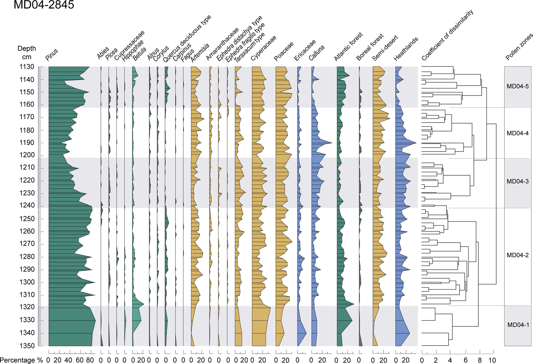
Figure 4. Pollen diagram of the MD04-2845 deep-sea core between 1335–1130 cm depth. From left to right: selected taxa, ecological groups (Atlantic forest, boreal forest, semi-desert plants, heathlands), and pollen zones, based on the clustering analysis and optical partitioning.
Zonation of the pollen diagram has been carried out by clusters or hierarchical groupings, constrained by a matrix of Euclidean distance between each sample (CONISS) (Grimm, Reference Grimm1987). This analysis was performed in the RStudio v. 1.2.5019 environment using the chclust program in the Rioja 0.9-21 package (Juggins, Reference Juggins2019).The number of significant pollen zones was determined using optimal partitioning with minimal sum-of-squares and broken-stick method using vegan v. 2.5-7 R-package (Oksanen et al., Reference Oksanen, Blanchet, Friendly, Kindt, Legendre, McGlinn and Minchin2020).
Principal Components Analysis (PCA) was applied to the pollen percentages to reduce the dimensionality for detecting climatic and environmental fluctuations. Of the 125 western European taxa (excluding Pinus, spores, and unidentified pollen grains), 72 taxa were retained to create the PCA without standardization. However, a matrix reduction was applied to select only major taxa with pollen percentages >6% in at least 5 samples (Fig. 5). Prior to the analysis, a Hellinger transformation was used (Legendre and Gallagher, Reference Legendre and Gallagher2001) to normalize the variance of the different taxa and make it therefore more suitable for Euclidean-based ordination methods, such as PCA. The Hellinger transformation was made using the R-vegan package (Oksanen et al., Reference Oksanen, Blanchet, Friendly, Kindt, Legendre, McGlinn and Minchin2020). Then, the values according the dimension scores were extracted for each sample. Another PCA taking into account the pollen zones, was made to determine the environmental significance of these pollen zones. The analysis was carried out in the RStudio environment with three packages—factoMineR v. 2.3 (Husson et al., Reference Husson, Lê and Pagès2017), factoextra v. 1.0.7 (Kassambara and Mundt, Reference Kassambara and Mundt2020), and paleoMAS v. 2.0.1 (Correa-Metrio et al., Reference Correa-Metrio, Urrego, Cabrera and Bush2012)—to extract and visualize the results of the multivariate data.
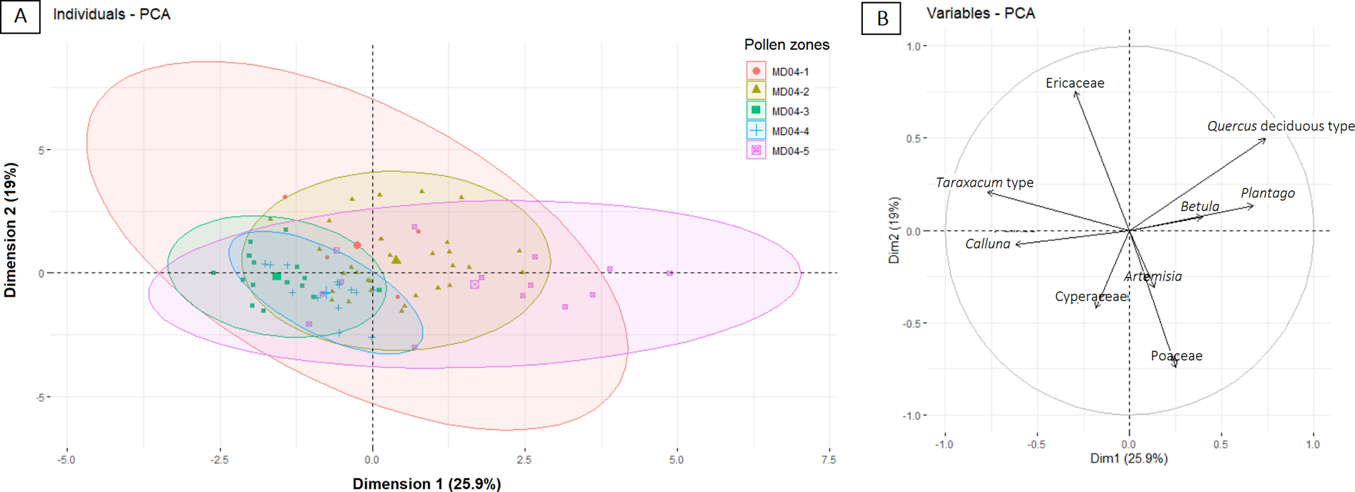
Figure 5. Principal Components Analysis (PCA) representing (a) pollen zones-based confidence ellipses, and (b) the 9 major taxa, with pollen percentages estimated to be >6% for at least 5 samples.
Analysis of foraminifera assemblages and SST quantitative reconstruction
Foraminifera assemblages of the MD04-2845 deep-sea core have been published previously (Sánchez Goñi et al., Reference Sánchez Goñi, Landais, Fletcher, Naughton and Desprat2008). Here, we present data for the three new samples (levels 1164, 1191, and 1226 cm), which were dated by 14C. The assemblages were analyzed in the >150 μm fraction of the same sample used for pollen analysis. Between 362–382 foraminifera were counted in these three samples. Quantitative values of seasonal and annual sea surface temperatures (SST) from planktonic foraminifera assemblages were reconstructed. This reconstruction used a paleoecological reconstruction program developed at the EPOC laboratory, based on modern analogues previously applied to this core (Sánchez Goñi et al., Reference Sánchez Goñi, Bard, Landais, Rossignol and d'Errico2013). This reconstruction relies on an extended modern database using North Atlantic and Mediterranean samples (1007 points).
Middle and Early Upper Paleolithic lithic techno-complexes
We have created a database initially containing 32 sites and ~300 previously published ages. To this database, we applied a series of qualitative methodological, taphonomic, and sampling criteria, from 0–3 following Guibert et al. (Reference Guibert, Bechtel, Bourguignon, Lenoir, Brenet, Couchoud and Delagnes2008), to select the most relevant ages (Excel file in Supplementary Information). The ages with index 3 are the most reliable and were integrated in the Bayesian models to reconstruct the temporal range of each LTC in each archaeological site. A model for each site was carried out with ChronoModel v. 2.0.18 (Lanos and Dufresne, Reference Lanos and Dufresne2019), taking into account the archaeostratigraphy between the different dated levels and using the most recent IntCal20 calibration curve (Reimer et al., Reference Reimer, Austin, Bard, Bayliss, Blackwell, Ramsey and Butzin2020). As for the age model of core MD04-2845, ChronoModel has the advantage of integrating multiple dated ages for the same event/sample and it is able to deal statistically with the outliers. Then the events were organized in phases (i.e., archaeological levels associated with a LTCs), only constrained stratigraphically within each site. We have chosen not to impose a chronological succession of these three LTCs, because although they could be stratified in the same site, they are not necessarily all contemporaneous from Aquitaine to northern Spain. Ages of archaeological levels below and above the targeted levels (i.e., Châtelperronian, Proto-Aurignacian, and Early Aurignacian) served as boundaries. However, the Early Aurignacian corpus needs further improvement, because only the ages corresponding to the Early Aurignacian levels of the sites delivering first Proto-Aurignacian and/or Châtelperronian layers have been integrated. The prior information included in the model is a stratigraphic order according to archaeological sequence. The posterior distributions and the HPD regions at 68.2% and 95.5% were approximated for each collection events and phases (Supplementary Information). We performed the age modeling for thirteen sites. However, among them, two sites provided only one age to include in the presentation and discussion of the results (Supplementary File 2).
RESULTS
Dating the Bay of Biscay core: results and improvements
The new 14C dates range from 33.9 ± 0.2 to 34.1 ± 0.2 14C yr BP (Table 4). The time interval corresponding to HS 4 in several North Atlantic cores (Elliot et al., Reference Elliot, Labeyrie, Bond, Cortijo, Turon, Tisnerat and Duplessy1998, Reference Elliot, Labeyrie, Dokken and Manthé2001, Reference Elliot, Labeyrie and Duplessy2002) is estimated between 33.9 ± 0.7 and 34.9 ± 1.1 14C yr BP, while farther south on the Iberian margin it is dated between 33.7–34.7 14C yr BP (Naughton et al., Reference Naughton, Sánchez Goñi, Kageyama, Bard, Duprat, Cortijo and Desprat2009) (Supplementary Figure 2, Supplementary Table 3). Chronological uncertainties for our AMS 14C dates range from 390–460 years (2σ error), and those based on the marine isotopic events have uncertainties between 817–1287 years (Wolff et al., Reference Wolff, Chappellaz, Blunier, Rasmussen, Svensson, Sanchez Goñi and Harrison2010; Sánchez Goñi et al., Reference Sánchez Goñi, Desprat, Daniau, Bassinot, Polanco-Martínez, Harrison and Allen2017). The new 14C ages appear to be statistically indistinguishable in terms of uncertainties (Table 4, Supplementary Fig. 2). These ages do not yield a consistent series of increasing age with increasing depth, perhaps due to variations in the marine age reservoir. Marine reservoir age simulations have highlighted variations in global mean marine reservoir ages of several hundreds of years, especially between ca. 42–38 ka close to the Laschamps (ca. 42.9–41.5 ka, Lascu et al., Reference Lascu, Feinberg, Dorale, Cheng and Edwards2016) geomagnetic excursion (Butzin et al., Reference Butzin, Heaton, Köhler and Lohmann2020; Heaton et al., Reference Heaton, Köhler, Butzin, Bard, Reimer, Austin and Ramsey2020).
Table 4. 14C dates of the three new samples and the other 14C ages used in this study and their calibration with Calib v.8.2.

The pIR-IR290 age obtained is 53.6 ± 3.4 ka (Table 2). This age, if considered with its uncertainty at 1 sigma, is younger than the other ages from other records for the HS 6, which is estimated between 64.0–60.0 ka based on the combination of 14C and isotopic event stratigraphy (Sánchez Goñi et al., Reference Sánchez Goñi, Bard, Landais, Rossignol and d'Errico2013). It is also younger compared to the age given by the Villars Cave speleothem (63.3–60.9 ± 0.8 ka; Genty et al., Reference Genty, Combourieu-Nebout, Peyron, Blamart, Wainer, Mansuri and Ghaleb2010). Moreover, GS 18, which would be the counterpart of HS 6 in Greenland, is dated at ca. 63.8–59.4 ka (Rasmussen et al., Reference Rasmussen, Bigler, Blockley, Blunier, Buchardt, Clausen, Cvijanovic, Rasmussen, Brauer, Moreno and Roche2014). However, in our record, there is no evidence that the grains were not completely bleached. HS 6 is a climatic phase encompassing a large input of IRD, which may have resulted in reworking, but we need to further investigate this hypothesis and increase the number of dated ages. This exploratory approach of dating marine sediments by luminescence and the preliminary pIR-IR290 age seems promising, which obviously needs to be confirmed with other luminescence testing and the dating of younger HSs (HS 1–4) whose ages can be compared with those obtained with 14C in order to validate the analytical strategy adopted.
The age-depth curve constructed with ArchaeoPhases, according to the hierarchical Bayesian model in ChronoModel, gives information on sedimentation rate based on ages and uncertainties (Fig. 3). Although the 14C and IRSL ages are younger, all the ages are slightly older in the depth-age model. This effect comes from the a priori stratigraphic constraint, which adjusts the ages by reducing uncertainties according to the stratigraphy of the sedimentary sequence. The sedimentation rate of the core is relatively constant from 70–40 ka, but it changes later on. The two dates around 1200 cm correspond to HS 4, which is marked by a different and rapid sedimentary process, such as an IRD deposition.
Vegetation and climate changes in SW France and its margin
Cluster analysis and broken-stick method applied to the pollen assemblage identified five pollen zones (MD04-1 to MD04-5), ranging from 1350–1130 cm deep (Fig. 4), ca. 49.8 ± 2.0 to 35.6 ± 0.8 ka (Fig. 6).
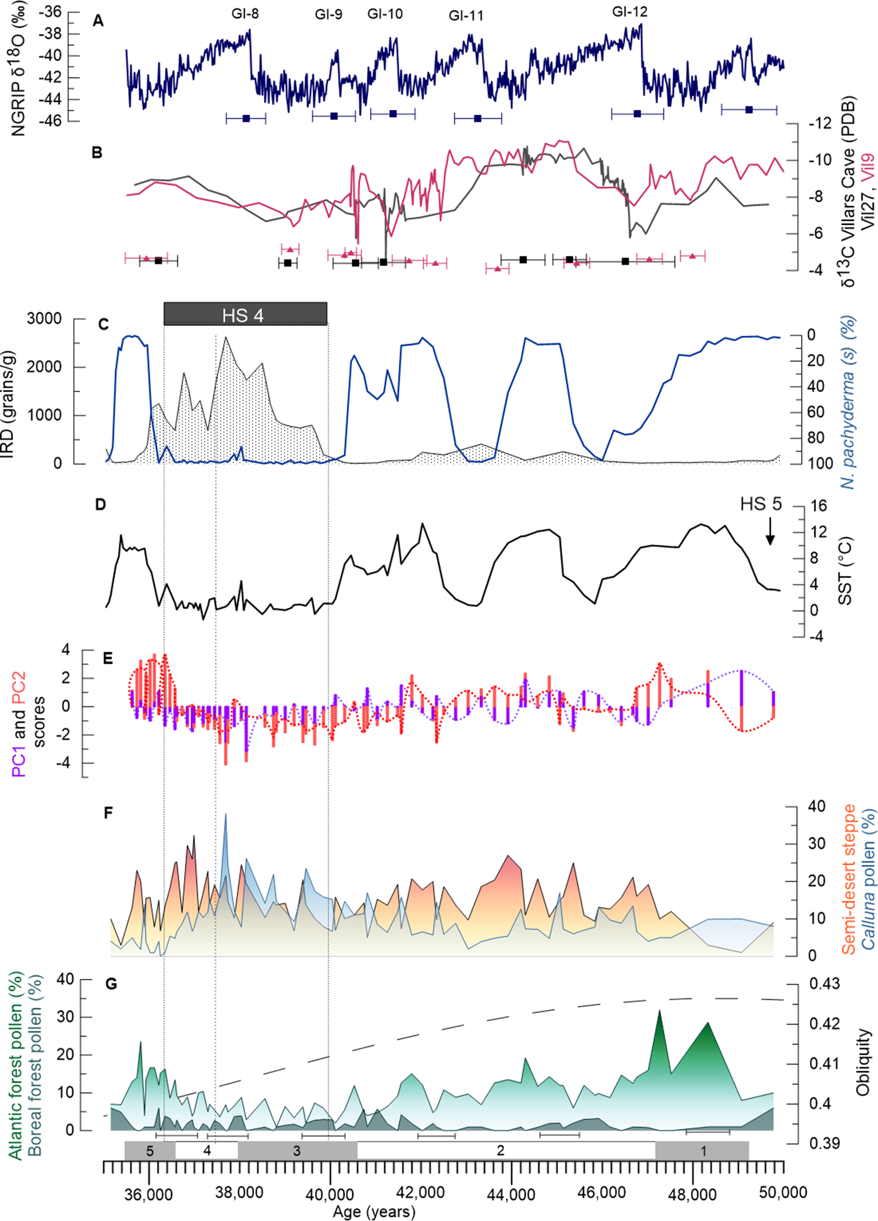
Figure 6. Oceanic and continental climatic multiproxies in the core, discussed from the bottom to the top of the figure. (F, G) Pollen percentages of Atlantic forest (degraded green), boreal forest (green), semi-desert plants (orange), Calluna (blue); obliquity curve (Laskar et al., Reference Laskar, Robutel, Joutel, Gastineau, Correia and Levrard2004) is represented with the temperate and boreal forest (G). (E) PC1 (purple) and PC2 (red) scores are represented in two different forms: purple/red bar charts and purple/red dotted curves. Dim1 (=PC1): the negative values correspond to dryness and positive to cold environments and Dim2 (=PC2) with positive scores to warm and negative scores to humid taxa (D), the annual sea surface temperature of Bay of Biscay (SST) derived from the polar foraminiferan Neogloboquadrina pachyderma (s) percentages, and quantity of IRD (C). The percentage scale of N. pachyderma (s) is reversed with respect to IRD. Villars stalagmites δ13C (B) Vil27 (gray) and Vil9 (red) and both of their chronological uncertainties are represented (only some uncertainties are shown; all uncertainties are available in Genty et al., Reference Genty, Blamart, Ouahdi, Gilmour, Baker, Jouzel and Van-Exter2003). (A) NorthGRIP δ18O curve (Rasmussen et al., Reference Rasmussen, Bigler, Blockley, Blunier, Buchardt, Clausen, Cvijanovic, Rasmussen, Brauer, Moreno and Roche2014) and the uncertainties for the GIs (Wolff et al., Reference Wolff, Chappellaz, Blunier, Rasmussen, Svensson, Sanchez Goñi and Harrison2010). Dotted rectangle (C–G) represents HS 4; dashed line indicates the separation between the two climatic phases within HS 4.
Zones MD04-1 and MD04-5 are characterized by an increase in the percentages of Atlantic forest taxa. The first zone (ca. 49.8–47.3 ka) is marked by a higher increase in temperate forest (29%) and, in particular, Betula (17%), Hippophae (3%), and deciduous Quercus (5%). Zone MD04-5 (ca. 36.7–35.6 ka) suggests a renewed forest expansion composed of Betula, Cupressaceae, deciduous Quercus, Alnus, Corylus, Carpinus, and Fagus, reflecting a warmer and wetter climate. Zone MD04-2 (ca. 47.3–40.9 ka) is characterized by steppe expansion, consisting of Artemisia, Amaranthaceae, Cyperaceae, and Poaceae, but also by forest expansion, as shown by increases of Betula, deciduous Quercus, Alnus, Corylus, and Carpinus. The boreal forest is represented in zones MD04-3 (ca. 40.9–38.3 ka), which is marked by the highest percentage of Abies in the entire sequence (4%), reflecting a cooling. This zone is also marked by a significant increase in humidity and a cold climate, as reflected by percentages of Calluna (e.g., 22% at ca. 38.7 ± 0.8 ka, 1209 cm; 23% at ca. 39.4 ± 0.9 ka, 1220 cm). On the contrary, MD04-4 (ca. 38.3–36.7 ka) is characterized by an increase in steppe taxa (32% at ca. 36.9 ± 0.9 ka, 1170 cm), especially Artemisia (19%), Poaceae (30%), and Cyperaceae (23%), along with the presence of boreal forest (2% of Picea), indicating a colder and drier climate. The beginning of the zone is marked by an increase in the percentages of Calluna species (38% at ca. 37.7 ± 0.8/0.81 ka, 1190 cm) reflecting a cold and humid climate. In this zone, E. fragilis is virtually absent. Within this zone, the percentages of Pinus decrease slightly around 38.2 ± 0.8 ka (1200 cm).
The results of the PCA explain 45% of the variance. The PCA identifies a first component (Fig. 5), that explains 25.9% of the variance characterized by deciduous Quercus and Betula with positive scores (warm), and herbaceous and shrub taxa such as Ericaceaea, Calluna, and Cyperaceae (cold) with negative scores. The second dimension, which explains 19% of the variance, is characterized by the positive scores of forest taxa, such as deciduous Quercus and Betula, and Ericaceae, which is a moist-loving taxon, while Artemisia, Poaceae, and Cyperaceae fall in the negative scores. In other words, variations of PC1 scores are used in this study as a warm/cold index and PC2 variations are used as a dry/wet and oceanic/continental proxy (Fig. 6E). Therefore, zones MD04-1 and MD04-5 represent relatively warm and wet climate, zones MD04-3 and MD04-4 colder and drier than the previous ones, and MD04-2 represents a relatively cold and wet climate. The warm and humid terrestrial phases are associated with the highest SST in the Bay of Biscay (Fig. 6D). The cold and dry terrestrial phases (Fig. 6F) are synchronous with cold SST, while the cold and humid phase is associated with SST oscillations.
Clustering analysis recognizes 14 pollen zones. However, optimal partitioning that gives the statistical significance of the zones has only detected 5 pollen zones and, therefore, D-O variability is not recorded from pollen percentages. However, in pollen zone MD04-2, two small increases in forest percentages are associated with two large SST increases that correspond with D-O 11 and D-O 10. Therefore, this variability, which was undetected by the optimal partitioning, seems to be real.
The chronology of the Middle to Upper Paleolithic technocomplexes
The ensemble of age models performed for each of the 11 sites in SW Europe (Fig. 7D, SI) show that the Châtelperronian, represented in this study by five sites mostly from the Aquitaine basin (i.e., Bordes-Fitte, Les Cottés, La Quina aval, and la Ferrassie) and Labeko-Koba (Wood et al., Reference Wood, Arrizabalaga, Camps, Fallon, Iriarte-Chiapusso, Jones, Maroto and de la2014) in the Spanish Basque country (Fig. 7D) spans from ca. 44.5 ka to ca. 40.1 ka. The Châtelperronian at la Quina aval and La Ferrassie could be the oldest (ca. 44 ka). The youngest ending time of this LTC would be, taking all uncertainties into account, ca. 40. 3 ka at Les Cottés and ca. 40.1 ka at La Ferrassie.

Figure 7. Comparison between environmental/climatic data and archaeological LTCs. (A) Bay of Biscay SST. (B, C) Pollen percentages of Atlantic forest (green), boreal forest (dark green), semi-desert steppe (orange), and Calluna species. (D) Representation of Middle to Upper Paleolithic transition LTCs. Modeled time ranges at 68.2% for Châtelperronian (green), Proto-Aurignacian (dark orange), and Early Aurignacian (yellow). The gray horizontal rectangle represents the only site of SE France. Dotted rectangle represents HS 4; dashed line indicates the separation between the two climatic phases within HS 4.
The Proto-Aurignacian, the first LTC attributed to the Upper Paleolithic and Homo sapiens, is found at Les Cottés, Isturitz (Barshay-Szmidt et al., Reference Barshay-Szmidt, Normand, Flas and Soulier2018) and Gatzarria (Barshay-Szmidt et al., Reference Barshay-Szmidt, Eizenberg and Deschamps2012) in the French Basque country, and at Labeko-Koba, Covalejos, and Cobrante in the Cantabrian of Spain (Marín-Arroyo et al., Reference Marín-Arroyo, Rios-Garaizar, Straus, Jones, Rasilla, de la, Morales, Richards, Altuna, Mariezkurrena and Ocio2018). It could have developed between ca. 44.2–41.4 ka at Isturitz and between 42.3–40.4 ka at Gatzarria. In northern Spain, it appeared in Covalejos between ca. 41.9–40.0 ka, in Labeko-Koba ca. 41.3–40.8 ka, ca. 41.3–39.1 ka in Cobrante, and in El Cuco between ca. 41.1–39.0 ka. In SE France, the Proto-Aurignacian, which is represented in our model only by Esquicho-Grapaou (Barshay-Szmidt et al., Reference Barshay-Szmidt, Bazile and Brugal2020), spans between ca. 42.9–38.0 ka. The youngest Proto-Aurignacian starting time is found at the Les Cottés site, which is dated between ca. 40.6–39.6 ka. The Proto-Aurignacian would be present in Western Europe first in northern Spain, then in SE France and the Aquitaine basin. However, this hypothesis is based on only a few well-dated sites from SW Europe.
The Proto-Aurignacian chronologically overlaps with the Châtelperronian. In SW France, taking into account the oldest and the most recent age from the Les Cottés and La Ferrassie sites, the overlap spans ca. 500 years. However, according to the techno-cultural attribution at the Bordes-Fitte site, which has the oldest presence of an Aurignacian occupation, this overlap would be ca. 1,100 years. Farther south, in the Basque country and Cantabrian region, the Châtelperronian overlaps with the Proto-Aurignacian for ca. 1,800 years, if we accept that the chronology of Isturitz is sufficiently reliable.
The Early Aurignacian is stratigraphically above the Proto-Aurignacian. It is represented by six sites located in SW France, the French and Spanish Basque country, and northern Spain. The Early Aurignacian is the oldest north of the Aquitaine basin at the Bordes-Fitte site, 41.2–40.1 ka, and in the Basque country at Isturitz, ca. 40.8–40.0 ka. It could have developed at Labeko-Koba between ca. 40.5–39.7 ka, and at Covalejos ca. 40.3–39.0 ka. In southwestern France, it appeared at Gatzarria between ca. 39.9–38.3 ka and ca. 39.4–38.8 ka at Les Cottés.
DISCUSSION
Climatic and environmental changes in SW France from GI 12–8 (ca. 50–36 ka)
The phases marked by the increase of Atlantic forest (Fig. 6G) are associated with the SST warming in the Bay of Biscay (Fig. 6C). Conversely, the phases dominated by semi-desert plants (Fig. 6F) are synchronous with cold SST. The chronologies of the four temperate phases punctuating the period between HS 5 and HS 4, does not correspond with the chronologies of GI 12–8, defined according to the Greenland δ18O record (Fig. 6A) (Rasmussen et al., Reference Rasmussen, Bigler, Blockley, Blunier, Buchardt, Clausen, Cvijanovic, Rasmussen, Brauer, Moreno and Roche2014). These SW European warming events show a difference of ca. 1,000 years from our age-depth model, compared to the onset of these GIs. This difference falls, however, within the uncertainties of the Greenland age model (800–1,300 years, Table 1) and the uncertainties of radiocarbon ages of this period. Atlantic forest pollen percentages indicate a progressive long-term decrease in the forest cover from GI 12–8, paralleling the decrease in obliquity (Fig. 6G), suggesting a warmer GI 12 (28%), compared to the other GIs. The high values of δ13C from two stalagmites in the Villars Cave (Genty et al., Reference Genty, Combourieu-Nebout, Peyron, Blamart, Wainer, Mansuri and Ghaleb2010) further indicate an increase in precipitation during GI 12 (Fig. 6A, B).
During HS 4, the SST was strongly imprinted by N. pachyderma (s) percentages, which decreased a few centuries before the increase of IRD (Fig. 6C). SST in the Bay of Biscay probably cooled contemporaneously with the first IRD discharges in the more northwestern regions. Therefore, and following the previous work of Sánchez Goñi et al. (Reference Sánchez Goñi, Turon, Eynaud and Gendreau2000), we define the time period of HS 4 in the Bay of Biscay between ca. 40.2–36.5 ka by using collectively the decrease of SST and the increases of N. pachyderma (s) and IRD. The age of HS 4, which is estimated between 40.2–38.3 cal BP (Sanchez Goñi and Harrison, Reference Sanchez Goñi, Harrison, Sanchez Goñi and Harrison2010), is based on the synthesis of 14C ages from North Atlantic deep-sea cores made by Elliot et al. (Reference Elliot, Labeyrie and Duplessy2002). The timing of the end of HS 4 given by the Bayesian age-depth model in core MD04-2845 using the new 14C age is ca. 1,500 years younger than that based on the North Atlantic 14C. However, taking into account all the uncertainties, our new age-model does not fundamentally contradict the traditional chronology of HS 4.
In SW France, HS 4 is composed of two climatic phases (Fig. 6). This subdivision into two phases was detected previously in a core from the northwestern Iberian margin (MD99-2331, 42°9'N, 9°69'W; Naughton et al., Reference Naughton, Sánchez Goñi, Kageyama, Bard, Duprat, Cortijo and Desprat2009). Our first phase (ca. 40.2–37.5 ka) is marked by the strongest iceberg discharges and is contemporaneous with the decrease of the Atlantic forest and maximum percentages of Calluna. This genus is a moisture and light-demanding plant whose development is favored by forest contraction (Naughton et al., Reference Naughton, Sánchez Goñi, Kageyama, Bard, Duprat, Cortijo and Desprat2009), reflecting an increase in humidity. Sea surface temperatures drop by ~7 ± 5°C. A slowdown in the growth of the Villars Cave speleothems is recorded during HS 4, also indicating a drastic decrease in precipitation in this region (Genty et al., Reference Genty, Blamart, Ouahdi, Gilmour, Baker, Jouzel and Van-Exter2003). Our second phase of HS 4 (ca. 37.5–36.4 ka) is synchronous with a moderate amount of IRD compared to the first phase, but the maximum of N. pachyderma (s) maintained low SSTs, between 0–2 ± 2°C in the Bay of Biscay.
Interestingly, within the first phase, SST and N. pachyderma (s) indicate a slight warming of 2 ± 3°C towards 38.2 ± 0.9 ka, which is associated with a small decrease in IRD. The percentages of N. pachyderma (s) fall to a value of 86.4% and SST increases by ~4 ± 3°C. Another deep-sea core off the Iberian Peninsula (MD95-2039, 40°34'N, 10°20'W) shows a slight warming associated with an increase in deciduous Quercus (Roucoux et al., Reference Roucoux, de Abreu, Shackleton, Tzedakis, Maddy, Long and Bridgland2005), which could indicate regional warming in the middle of HS 4 between 40–45°N. In the Bay of Biscay, the percentage of deciduous Quercus (1%) remains low, but the Atlantic forest reaches almost 9% due to a 3% increase in Alnus, 2% in Corylus, and 1% in Betula and Carpinus.
HS 4 is thus divided into two different climatic and environmental phases in the eastern North Atlantic region between 40°N and 45°N: a first phase, associated with the maximum amount of IRD and marked by extreme cooling and wet conditions; and a second phase, characterized by a drier and colder climate showing a warming trend. However, unlike the cores from the Iberian margin, where the first phase is considered to be the coldest one, the two phases in the Bay of Biscay are relatively similar in terms of forest cover and oceanic temperatures throughout HS 4.
Climatic and environmental changes: triggers for technological adaptations?
The studies of SW France archaeological sites played a major role in the definition of both Middle and Upper Paleolithic cultures. The oldest appearance of the Châtelperronian at la Quina aval and La Ferrassie (ca. 44 ka) could be contemporaneous with GS 11 (Fig. 7). The presence of Châtelperronian at La Ferrassie would be the earliest presence in SW France, well before the Châtelperronian from Arcy-sur-Cure (Talamo et al., Reference Talamo, Aldeias, Goldberg, Chiotti, Dibble, Guérin and Hublin2020). Farther north, at Bordes-Fitte rockshelter and Les Cottés Cave, it might have begun between 42.9–41.5 ka, corresponding perhaps to the end of GS 11. At Labeko-Koba, the most southern site, the Châtelperronian is dated between 43.0–41.6 ka and encompasses the end of GS 11. Depending on the region, the Châtelperronian developed since the end of GS 11 or during GS 10. However, in SW France and northern Spain, the Châtelperronian does not appear beyond the beginning of HS 4. The last age of the Châtelperronian, which is associated with the last Neanderthals, indicates that their disappearance would have occurred in this region at the same time as the start of HS4.
The Proto-Aurignacian could have appeared in SW and SE France, as well as in northern Spain, around the GS 10/GS 9 transition, which is marked by the expansion of an open forest with steppe-like elements. Shao et al. (Reference Shao, Limberg, Klein, Wegener, Schmidt, Weniger, Hense and Rostami2021), using a global climate model, developed a human-existence model combining climate data with archaeological sites to reconstruct patterns of Aurignacian dispersal. The earliest Aurignacian dispersal in Europe started before 45 ka (Hublin et al., Reference Hublin, Sirakov, Aldeias, Bailey, Bard, Delvigne and Endarova2020). The recent discovery in Mandrin Cave (Rhone valley) of a tooth that belonged to H. sapiens, has highlighted its presence in Western Europe before 50 ka (Slimak et al., Reference Slimak, Zanolli, Higham, Frouin, Schwenninger, Arnold and Demuro2022).
In Proto-Aurignacian levels, reindeer dominates the faunal assemblages in Charentes and Périgord, while horses and Bovidae are dominant in the Pyrenees (Discamps et al., Reference Discamps, Soulier, Bachellerie, Bordes, Castel, Morin, Thiébaut, Costamagno and Claud2010; Soressi et al., Reference Soressi, Roussel, Rendu, Primault, Rigaud, Texier, Richter, Buisson-Catil and Primault2010; Barshay-Szmidt et al., Reference Barshay-Szmidt, Normand, Flas and Soulier2018). Around GS 9, steppe and, to a lesser extent, boreal forest could explain the strong presence of reindeer; bison, and horses in both regions. Progressive reduction of forest cover from GS 9 to HS 4 probably also had an effect on modern human migration (Badino et al., Reference Badino, Pini, Ravazzi, Margaritora, Arrighi and Bortolini2020). So far, our age modeling suggests that the appearance of Homo sapiens would have occurred first in SW France, with migration later in SE France, arriving in northern Spain at ca. 41.8 ka. However, Talamo et al. (Reference Talamo, Aldeias, Goldberg, Chiotti, Dibble, Guérin and Hublin2020), using another age-modeling approach (IntCal 13, Reimer et al., Reference Reimer, Bard, Bayliss, Beck, Blackwell, Ramsey and Buck2013, and OxCal, Ramsey, Reference Ramsey2009) obtained an age for Isturitz that is younger than our model, and, in this case, Homo sapiens would have arrived in SE France before before farther west. Their scenario is consistent with the recent dating of the Proto-Aurignacian at Mandrin Cave, the beginning of which is dated between 43.3–42.2 ka (Slimak et al., Reference Slimak, Zanolli, Higham, Frouin, Schwenninger, Arnold and Demuro2022).
The first occurrences of the Early Aurignacian happened during GS 9 and the onset of HS 4 in Gatzarria and Les Cottés. The Early Aurignacian persisted during the beginning of HS 4. The faunal record also indicates a dominance of open and cold environmental faunal species in the Early Aurignacian (Discamps et al., Reference Discamps, Soulier, Bachellerie, Bordes, Castel, Morin, Thiébaut, Costamagno and Claud2010). Interestingly, within this LTC, a geographical difference also seems to emerge between the north and south, which are dominated by reindeer and by horses and Bovidae, respectively (Barshay-Szmidt et al., Reference Barshay-Szmidt, Normand, Flas and Soulier2018). Unfortunately, no pollen data exists documenting a difference in the vegetation between the north and the south of SW France and northern Spain. The transition between Proto-Aurignacian and Early Aurignacian would overlap GS 9 and the first phase of HS 4.
The overlap between Châtelperronian and Proto-Aurignacian could be ca. 3,300 years between SW France and northern Spain. This overlap suggests a coexistence of several millennia between Neanderthal and modern groups (Marín-Arroyo et al., Reference Marín-Arroyo, Rios-Garaizar, Straus, Jones, Rasilla, de la, Morales, Richards, Altuna, Mariezkurrena and Ocio2018), and interbreeding between Neanderthals and ancestors of non-African modern humans (Green et al., Reference Green, Krause, Briggs, Maricic, Stenzel, Kircher and Patterson2010). In recent years, genetic studies show the coexistence of Neanderthals and Homo sapiens by admixture from Neanderthals into ancestors of present populations in several regions of the world (Green et al., Reference Green, Krause, Briggs, Maricic, Stenzel, Kircher and Patterson2010; Prüfer et al., Reference Prüfer, Racimo, Patterson, Jay, Sankararaman, Sawyer and Heinze2014, Reference Prüfer, Posth, Yu, Stoessel, Spyrou, Deviese and Mattonai2021; Fu et al., Reference Fu, Hajdinjak, Moldovan, Constantin, Mallick, Skoglund and Patterson2015; Bokelmann et al., Reference Bokelmann, Hajdinjak, Peyrégne, Brace, Essel, Filippo and Glocke2019; Bergström et al., Reference Bergström, McCarthy, Hui, Almarri, Ayub, Danecek and Chen2020) either through a single (Sankararaman et al., Reference Sankararaman, Patterson, Li, Pääbo and Reich2012; Bergström et al., Reference Bergström, McCarthy, Hui, Almarri, Ayub, Danecek and Chen2020) or multiple episodes of gene flow (Prüfer et al., Reference Prüfer, Racimo, Patterson, Jay, Sankararaman, Sawyer and Heinze2014; Vernot and Akey, Reference Vernot and Akey2015; Villanea and Schraiber, Reference Villanea and Schraiber2019; Hublin et al., Reference Hublin, Sirakov, Aldeias, Bailey, Bard, Delvigne and Endarova2020).
Western Europe experienced strong climate changes, which affected the environments and the food resources of Neanderthals and modern humans. So far, the archaeological records show that the transition between each of the LTCs between 44–36 ka encompassed several warming and cooling events, and that the same LTC is not synchronous throughout SW France and northern Spain. However, the late Neanderthal LTC seems to have developed in a moderately forested landscape, while modern humans developed in successively more open environments.
Comparison of both paleoclimatic and archaeological records aiming to detect potential synchronies is a complex process due to the age resolution and typo-technological definitions. Therefore, the chronology of the Middle-Upper Paleolithic transition is still not conclusive and needs to be improved by enlarging the database and pursuing the chronological modeling approach using Bayesian statistics.
Our study further suggests that the disappearance of Neanderthals does not seem to be directly related to climate-driven environmental changes, although the Châtelperronian ended in several sites before HS 4 onset. However, uncertainty in determining the age of HS 4 and the apparent young age of this event in this marine record reveal that there is an uncertainty making it difficult to assume a relationship between the end of the Châtelperronian and HS 4 onset. In SW France and the Cantabrian regions, the late Neanderthals survived several warming and cooling events, but just disappeared after the first LTCs associated with modern humans are recorded. Furthermore, the progressive increase of open environments from ca. 50–40 ka would have been favorable to expansion of modern humans, who could have been well adapted to the steppe. They could have competed with the late Neanderthals for the same ecological niches, causing their regional disappearance. Our new data are in line with previous modeling studies showing that Neanderthal disappearance can only be achieved when modern humans are chosen in the model as being more adapted in the exploitation of food resources and hunting technology compared to Neanderthals (Sepulchre et al., Reference Sepulchre, Ramstein, Kageyama, Vanhaeren, Krinner, Sánchez-Goñi and d'Errico2007; Banks et al., Reference Banks, d'Errico, Peterson, Kageyama, Sima and Sánchez-Goñi2008; Columbu et al., Reference Columbu, Chiarini, Spötl, Benazzi, Hellstrom, Cheng and De Waele2020; Timmermann, Reference Timmermann2020).
CONCLUSIONS
The high resolution pollen study of the MD04-2845 deep-sea core retrieved from the Bay of Biscay precisely identified the effect of climate changes from D-O 12–8 cycles and HS 4 in SW France. HS 4, defined on the basis of increases in IRD and N. pachyderma (s), is characterized by two distinct climatic phases: a first wet and cold phase and a second drier and colder phase. In the long term, a progressive decrease in the Atlantic forest and concomitant expansion of open environments is recorded from 50–40 ka. From a chronological point of view, IRSL dating results on the MD04-2845 deep-sea core seems promising, and future sample dating should confirm its application for sedimentary sequences older than the limits of radiocarbon dating. In addition, Bayesian statistics for both paleoclimatic and archaeological data from the westernmost part of Europe allowed us to improve the identification of potential synchronies. This critical work on an archaeological database and chronological modeling could be applied to Mousterian (older) LTCs to better characterize their variability over the Middle Paleolithic.
This comparison shows that changes in LTCs during the Middle to Upper Paleolithic transition do not correspond with punctual vegetation and climate changes. In contrast, progressive opening of the regional landscape seems to have provided the context for the replacement of Neanderthals by modern humans, which lasted several millennia during which potential interbreeding and cultural changes occurred. Finally, our data suggest that climate changes did not directly cause the disappearance of Neanderthal. That disappearance was probably the result of competition with Homo sapiens for the same ecological niches.
Supplementary Material
The supplementary material for this article can be found at https://doi.org/10.1017/qua.2022.21
Acknowledgments
This work was initially funded by the New Aquitaine Region NATCH scientific project (Neanderthalenses aquitanensis: Territoires, Chronologie, Humanité, co-dir. J.Ph. Faivre, C. Lahaye, B. Maureille), and continued during a doctoral contract n°12-18 (Ecole Doctorale Montaigne Humanités), and by financial support from the French Research National Agency under the Investissements d'Avenir Program (ANR-10-LABX-52). 14C dating was carried out with the support of ERC Advanced Grant TRACSYMBOLS no. 249587. We thank the members of UMR 5805 EPOC and UMR 6034 Archeosciences Bordeaux for their technical assistance (L. Devaux, M. Georget, M.-H. Castera, O. Thier, and I. Billy; J. Faure). Thanks to D. Genty and S. Salonen for their help and interesting discussions. We thank the three anonymous referees for their insightful comments to revise this paper.


