INTRODUCTION
The role of the tropics in climate change has garnered significant attention in recent decades (e.g., Cane, Reference Cane1998; Seltzer, Reference Seltzer2001; Chiang, Reference Chiang2009; Jomelli et al., Reference Jomelli, Favier, Vuille, Braucher, Martin, Blard and Colose2014). However, debate still exists on the nature of climate change in the tropics and on the connections between drivers of climate variations in the tropics and those in the middle to high latitudes (e.g., Seltzer, Reference Seltzer2001; Farber et al., Reference Farber, Hancock, Finkel and Rodbell2005; Smith et al., Reference Smith, Seltzer, Farber, Rodbell and Finkel2005, Reference Smith, Mark and Rodbell2008; Licciardi et al., Reference Licciardi, Schaefer, Taffart and Lund2009; Jomelli et al., Reference Jomelli, Favier, Vuille, Braucher, Martin, Blard and Colose2014). Glaciers in tropical mountains are highly sensitive to climate change (Kaser and Osmaston, Reference Kaser and Osmaston2002; Benn et al., Reference Benn, Owen, Osmaston, Seltzer, Porter and Mark2005). Thus, constraining the timing and extent of past glacial fluctuations in tropical mountains is of key importance for understanding tropical paleoclimate trends and their forcing mechanisms. However, it has been difficult to constrain ages of the landforms left behind by past glaciers, so exploiting the climate information they contain has been difficult or impossible. The development of cosmogenic nuclide surface exposure dating (e.g., Gosse and Phillips, Reference Gosse and Phillips2001; Li and Harbor, Reference Li, Harbor, Ferrari and Guiseppie2009) provides a unique opportunity to date glacial landforms and thereby address important paleoclimate issues, including whether glacial advances were synchronous or asynchronous between the tropics and middle/high latitudes (e.g., Gillespie and Molnar, Reference Gillespie and Molnar1995; Smith et al., Reference Smith, Seltzer, Farber, Rodbell and Finkel2005, Reference Smith, Mark and Rodbell2008; Schaefer et al., Reference Schaefer, Denton, Barrell, Ivy-Ochs, Kubik, Andersen, Phillips, Lowell and Schluchter2006, Reference Schaefer, Denton, Kaplan, Putnam, Finkel, Barrell and Andersen2009; Clark et al., Reference Clark, McCabe, Clark, McCarron, Freeman, Maden and Xu2009; Licciardi et al., Reference Licciardi, Schaefer, Taffart and Lund2009; Smith and Rodbell, Reference Smith and Rodbell2010; Jomelli et al., Reference Jomelli, Favier, Vuille, Braucher, Martin, Blard and Colose2014).
With their great combined latitudinal extent, the mountain ranges of tropical America—from the central Mexican volcanoes through Central America and southward through the Andes to Bolivia—are ideal places to reconstruct past glacier fluctuations in the tropics and to examine the climatic linkages between the tropics and middle/high latitudes (Hastenrath, Reference Hastenrath2009). To date, most studies using cosmogenic nuclides to constrain glacial chronologies are from Southern Hemisphere sites in the Peruvian and Bolivian Andes (mainly 10Be), such as the Junin Plain (Smith et al., Reference Smith, Seltzer, Farber, Rodbell and Finkel2005, Reference Smith, Mark and Rodbell2008), the Cordillera Blanca (Farber et al., Reference Farber, Hancock, Finkel and Rodbell2005; Glasser et al., Reference Glasser, Clemmens, Schnabel, Fenton and McHargue2009; Smith and Rodbell, Reference Smith and Rodbell2010), the Cordillera Vicabamba (Licciardi et al., Reference Licciardi, Schaefer, Taffart and Lund2009), the Cordillera Huayhuash (Hall et al., Reference Hall, Farber, Ramage, Rodbell, Finkel, Smith, Mark and Kassel2009), the Nevado Coropuna (Bromley et al., Reference Bromley, Schaefer, Winckler, Hall, Todd and Rademaker2009), and the Cordillera Real (Smith et al., Reference Smith, Lowell, Owen and Caffee2011). In the northern neotropics, cosmogenic nuclide ages are available from the central Mexican volcanoes (36Cl; Vázquez-Selem and Heine, Reference Vázquez-Selem, Heine, Ehlers and Gibbard2004) and the Merida Andes, Venezuela (10Be; Wesnousky et al., Reference Wesnousky, Aranguren, Rengifo, Owen, Caffee, Murari and Perez2012; Carcaillet et al., Reference Carcaillet, Angel, Carrillo, Audemard and Beck2013; Angel et al., Reference Angel, Audemard, Carcaillet, Carrillo, Beck and Audin2016). Glacial features have been documented and mapped in the Sierra de los Cuchumatanes, Guatemala, most thoroughly by Roy and Lachniet (Reference Roy and Lachniet2010), but no radiometric ages are available (Lachniet and Roy, Reference Lachniet, Roy, Ehlers, Gibbard and Hughes2011). In Costa Rica, dating has focused on basal organic sediments in glacial lakes within the cirques (Orvis and Horn, Reference Orvis and Horn2000), which provide the minimum ages of the last deglaciation. Knowledge of glacial chronologies in the northern neotropics is thus incomplete, hindering efforts to understand the role of the tropics in triggering, transmitting, and amplifying interhemispheric climate signals.
In the work reported here, we constrained the timing of glacial events around Cerro Chirripó in the Cordillera de Talamanca, Costa Rica, using cosmogenic 36Cl surface exposure dating. This work establishes a glacial chronology in this key area of Central America that can be used to test whether glacial events in this area were synchronous with those documented in the tropical Andes and Central Mexico. The findings from this research provide important insights into paleoclimate and environmental changes in tropical America.
STUDY AREA
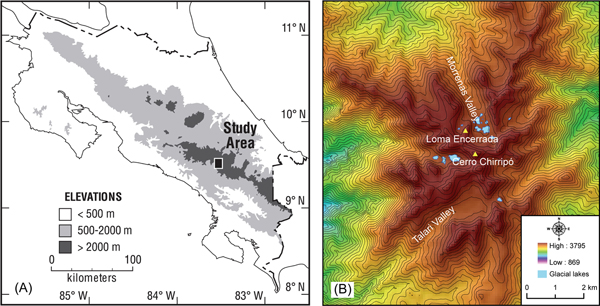
Our study area is the small upland massif surrounding Cerro Chirripó (3819 meters above sea level [m asl]; 9°29.05'N, 83°29.32'W) on the northwestern end of the Cordillera de Talamanca in Costa Rica (Fig. 1). Cerro Chirripó, the highest point on the massif and in all of Costa Rica, is a glacial horn and a popular hiking destination near the center of the remote Chirripó National Park. The peaks and upland valleys of the Chirripó massif extend above the regional treeline and are covered by neotropical páramo vegetation dominated by the miniature bamboo Chusquea subtessellata, other grasses, and shrubs (Kappelle and Horn, Reference Kappelle and Horn2005, Reference Kappelle, Horn and Kappelle2016). The Cerro Páramo meteorologic station (3466 m asl; 9°33.60'N, 83°45.18'W), about 30 km west of Cerro Chirripó in the páramo of the Buenavista massif, recorded a mean annual precipitation of 2581 mm and a mean annual temperature of 8.5°C between 1971 and 2000 (Lane et al., Reference Lane, Horn, Mora, Orvis and Finkelstein2011). Snow has not been officially recorded in Costa Rica, though the Swiss geographer and botanist Henri Pittier reported a mixture of rain and snow, with no accumulation, on Cerro Buenavista in January 1897 (Herrera, Reference Herrera, Kappelle and Horn2005; Castillo-Muñoz, Reference Castillo-Muñoz2010).

Figure 1. (color online) (A) Map of Costa Rica showing location of Chirripó massif in the Cordillera de Talamanca. (B) Shaded relief of the study area derived using the 90 m Shuttle Radar Topography Mission digital elevation model (http://srtm.csi.cgiar.org, last accessed on July 20, 2018). The Morrenas Valley is located on the north flank and the Talari Valley on the southwest flank of the massif. The contour interval is 50 m.
The Chirripó and Buenavista massifs preserve important records of Pleistocene tropical climate in glacial landforms (Hastenrath, Reference Hastenrath1973; Orvis and Horn, Reference Orvis and Horn2000; Lachniet and Seltzer, Reference Lachniet and Seltzer2002; Lachniet, Reference Lachniet, Ehlers and Gibbard2004, Reference Lachniet, Bundschuh and Alvarado2007; Lachniet and Vazquéz-Selem, Reference Lachniet and Vázquez-Selem2005; Castillo-Muñoz, Reference Castillo-Muñoz2010) and lake sediments (Horn, Reference Horn1990, Reference Horn1993; Lane et al., Reference Lane, Horn, Mora, Orvis and Finkelstein2011; Lane and Horn, Reference Lane and Horn2013), as well as in highland bogs (Martin, Reference Martin1964; Islebe and Hooghiemstra, Reference Islebe and Hooghiemstra1997) and paleosols (Driese et al., Reference Driese, Orvis, Horn, Li and Jennings2007) beyond the ice limit. Glacial features near Cerro Chirripó, where they are most extensive, were first reported by Weyl (Reference Weyl1956a, Reference Weyl1956b). Hastenrath (Reference Hastenrath1973) identified specific moraine complexes and speculated on ages but was unable to find suitable material in moraines for dating. Bergoeing (Reference Bergoeing1977) interpreted glacial geomorphology from aerial photographs, Barquero and Ellenberg (Reference Barquero and Ellenberg1983, Reference Barquero and Ellenberg1986) mapped glacial features from fieldwork and aerial photograph analyses, and Wunsch et al. (Reference Wunsch, Calvo, Willscher and Seyfried1999) mapped and interpreted glacial features along with rock types from fieldwork. Horn (Reference Horn1990) inferred the timing of deglaciation from radiocarbon dating of basal organic and transitional sediments in the largest lake in the Morrenas Valley. Orvis and Horn (Reference Orvis and Horn2000) obtained sediment cores and radiocarbon dates from additional lakes, mapped moraines, and reconstructed equilibrium line altitudes (ELAs) and past ice extents corresponding to these moraines in the Morrenas Valley. Lachniet and Seltzer (Reference Lachniet and Seltzer2002) and Lachniet and Vázquez-Selem (Reference Lachniet and Vázquez-Selem2005) investigated and mapped glacial features across the massif, reconstructed ELAs, and examined the weathering of boulders on moraines attributed to two different glacial stages. Orvis and Horn (Reference Orvis and Horn2000) and Lachniet and Seltzer (Reference Lachniet and Seltzer2002) both proposed that an ice cap covered the Chirripó massif during the late Pleistocene; Lachniet and Seltzer (Reference Lachniet and Seltzer2002) also presented evidence on past ice extent on two other high peaks in the Cordillera de Talamanca—Cerro Buenavista (also called Cerro de la Muerte), along the Inter-American Highway crossing to the west of Cerro Chirripó, and Cerro Kamuk near the border with Panama.
Some uncertainty exists as to which climate factors most affected glacial advance and retreat in this area. Hastenrath (Reference Hastenrath2009) suggested that the ELA for mountain glaciers in the inner humid tropics may be more sensitive to temperature variation than to precipitation variation. Lachniet and Seltzer (Reference Lachniet and Seltzer2002) conjectured that ELA temperature depressions in Costa Rica during the late Quaternary might be associated with a steeper lapse rate resulting from drier climate conditions produced by an equatorward restriction or weakening of the Intertropical Convergence Zone. From the reconstruction of ELAs and past glacial extents, Orvis and Horn (Reference Orvis and Horn2000) speculated that both temperature (cold) and precipitation (drier or wetter) conditions influenced late Quaternary glacial fluctuations in the Cordillera de Talamanca.
This study focuses on two valleys next to Cerro Chirripó: the Morrenas and Talari Valleys. Bedrock consists of dacitic volcanic rocks, sedimentary rocks, and crystalline granitoid intrusives (Wunsch et al., Reference Wunsch, Calvo, Willscher and Seyfried1999). The Morrenas Valley is a formerly glaciated, north/northwest-facing valley adjacent to the Chirripó headwall. Within the cirque, glacial lakes and moraines create a hummocky terrain surrounded by valley walls with limited vegetation growth on top of bedrock (Horn et al., Reference Horn, Orvis, Haberyan, Kappelle and Horn2005). The sizes of the lakes vary, but the largest measures 5.6 ha and 8.3 m deep (Horn et al., Reference Horn, Orvis, Haberyan, Kappelle and Horn2005). The gradient of the valley floor steepens downvalley from the cirque. The Talari Valley faces southwest. Its cirque also has a hummocky terrain (but without glacial lakes), and the valley gradient steepens downvalley from the cirque. On the northwest side of the upper Talari Valley, freeze-thaw processes have produced solifluction terraces in the ablation till mantling the slope (Lachniet and Seltzer, Reference Lachniet and Seltzer2002).
Orvis and Horn (Reference Orvis and Horn2000) mapped four moraine complexes in the Morrenas Valley: Chirripó IV (oldest), III, II, and I (youngest) (Fig. 2). The Chirripó IV moraine (M-4 in Fig. 2) corresponds to the oldest and largest glacial advance in this valley, and it is ~3.2 km downvalley (reaches to 3310 m asl) from the Chirripó headwall. The Chirripó III moraine (M-3 in Fig. 2) is ~0.9 km upvalley from the Chirripó IV moraine (2.3 km from Chirripó headwall). The Chirripó II moraine (M-2 in Fig. 2) is ~0.8 km upvalley from the Chirripó III moraine (1.6 km from Chirripó headwall). The Chirripó I moraine complex (M-1 in Fig. 2) is within the cirque and includes a set of moraines that surround glacial lakes. We carried out cosmogenic nuclide surface exposure dating of moraines from all four complexes.

Figure 2. Geomorphological map of the study area, including moraines, till deposits, glacial lakes, and the sample sites in the Morrenas and Talari Valleys. Red dots show the sample sites for 36Cl surface exposure dating. Samples CS-0 to CS-5 were collected from the cirque of the Morrenas Valley in 1998. Each dot on other moraines (M-4, M-3, and M-2 in the Morrenas Valley and T-II and T-I in the Talari Valley) represents a set of 10 samples collected from each site in 2000 and 2001. The 36Cl exposure ages (ka) are also marked for each sample and sample site. The ages in red font are treated as outliers. The white box represents the extent of Figure 5A. (For interpretation of the references to color in this figure legend, the reader is referred to the web version of this article.)
We also investigated two moraines in the Talari Valley. The lower moraine (T-II in Fig. 2) is ~2.6 km downvalley (reaches to 3349 m asl) from the valley headwall. The upper moraine (T-I in Fig. 2; reaches to 3357 m asl) is very close to and just about 0.3 km upvalley from the lower moraine. Lachniet and Seltzer (Reference Lachniet and Seltzer2002) examined moraines and other glacial features throughout the Chirripó massif and identified three moraine groups in the Morrenas and Talari Valleys (Talamanca, Chirripó, and Talari), corresponding to the Chirripó IV–II moraines of Orvis and Horn (Reference Orvis and Horn2000). The two moraines we studied in the Talari Valley (T-II and T-I) correspond to the Talamanca and Chirripó moraines, respectively, described by Lachniet and Seltzer (Reference Lachniet and Seltzer2002).
Radiocarbon ages from lake sediment cores in the Morrenas Valley indicated that the last glacial advance could correspond in time to the Younger Dryas, with this advance followed by complete deglaciation sometime after 12.4 ka cal BP but before 9.7 ka cal BP (Orvis and Horn, Reference Orvis and Horn2000). These radiocarbon dates on basal lake sediment correspond to the youngest moraine complex (Chirripó I) identified by Orvis and Horn (Reference Orvis and Horn2000) and were the only dates available to the researchers. Like Hastenrath (Reference Hastenrath1973), Orvis and Horn (Reference Orvis and Horn2000) were unable to secure organic material from moraines for radiocarbon dating. Based on studies in Mexico and South America, the researchers suggested a polystage interpretation in which the Chirripó II moraine complex was associated with Marine Oxygen Isotope Stage (MIS) 2, and they tentatively correlated Chirripó III with MIS 4 and Chirripó IV with MIS 6. Lachniet and Seltzer (Reference Lachniet and Seltzer2002) measured pedestal heights of quartz veins on boulders and bedrock associated with their Chirripó stage (equivalent to Orvis and Horn's Chirripó III) and Talamanca stage (Chirripó IV), and from this work, they inferred that these two stages might be only a few thousand years different in age. They suggested that their Talari (Chirripó II) moraines could represent features formed during small advances or recessions during the Chirripó (Chirripó III) phase, as interpreted by Hastenrath (Reference Hastenrath1973). Wunsch et al. (Reference Wunsch, Calvo, Willscher and Seyfried1999), in a study not available to Orvis and Horn (Reference Orvis and Horn2000) or Lachniet and Seltzer (Reference Lachniet and Seltzer2002), classified all moraines except the oldest set as recessional, describing them as a series of “backstepping terminal and lateral moraines” formed by “oscillations during the backmelting stage” (Wunsch et al. Reference Wunsch, Calvo, Willscher and Seyfried1999, p. 194). However, until the study we describe here, no absolute dating results were available from moraines in the Chirripó highlands to test these competing ideas.
METHODS
Sample collection, processing, and measurement
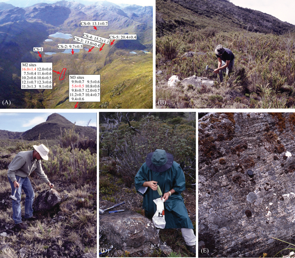
On three expeditions to the Chirripó highlands in 1998, 2000, and 2001, we collected 56 boulder samples from moraines for cosmogenic 36Cl surface exposure dating. Six samples were collected from moraines within the cirque of the Morrenas Valley (M-1) in 1998 (CS-0 to 5) to test the feasibility of using 36Cl surface exposure dating in this area (Figs. 2 and 3A). Then, 50 samples were collected from three moraines (M-4, M-3, and M-2) below the cirque in the Morrenas Valley and from two moraines in the Talari Valley (T-II and T-I) in 2000 and 2001 (10 samples from each moraine; Figs. 2 and 3). Chemical compositions of the samples we collected plot as diorite on a TAS (Total Alkali Silica) diagram for plutonic rocks (Rippington et al., Reference Rippington, Cunningham and England2008). Approximately 1000 g of rock fragments was chipped from the surface of each selected boulder using hammers and chisels. We measured the latitude, longitude, and altitude information individually using a GPS unit for the six samples (CS-0 to 5) within the cirque of the Morrenas Valley. For other samples, we measured GPS locations of the bottom and the top of each set along the moraine ridge and used the average GPS location for all samples in each set. We did not keep individual notes, such as the size and height above the ground, on individual boulders. All boulders we collected were not ideally large and landmark boulders, but they were the best we could find on top of each moraine.

Figure 3. (color online) (A) Photo taken from a small plane, looking south up the Morrenas Valley (marked with the locations and 36Cl exposure ages [ka] of the samples within the cirque [CS-0 to 5] collected in 1998 and of the M-2 and M-3 sample sites). (B–D) Field photos of sampling boulders for 36Cl surface exposure dating. (E) A bedrock surface with glacial striations in the Talari Valley. Photo credits: Luis González Arce, Carol Harden, and Sally Horn.
Samples were processed at Purdue Rare Isotope Measurement Laboratory (PRIME Lab), Purdue University, and in the cosmogenic sample preparation lab in the Laboratory of Paleoenvironmental Research at the University of Tennessee. We used the whole rock for the 36Cl analysis. Each sample was first crushed and then leached to remove organic matter. After that, 15 g of well-mixed material from each sample was sent to Minerals Analytical at SGS Canada for elemental analysis, and approximately 30 g was dissolved using low Cl HF. About 1.0 mg 35Cl spike carrier was added to each sample to measure the 35Cl/37Cl and 36Cl/35Cl ratios. Then, silver nitrate (AgNO3) was added to precipitate silver chloride (AgCl). Each sample was then eluted through anion exchange chromatography to purify the silver chloride. The purified silver chloride of each sample was loaded into a holder (Cu covered by AgBr) and sent to the PRIME Lab for accelerator mass spectrometry (AMS) measurement.
Exposure age calculations
Cosmogenic 36Cl is produced by multiple reaction pathways: spallation and muon-induced reactions of Ca, K, Fe, and Ti and thermal and epithermal neutron-capture reactions of 35Cl (Marrero et al., Reference Marrero, Phillips, Borchers, Lifton, Aumer and Balco2016a, Reference Marrero, Phillips, Caffee and Gosse2016b). The spallation is caused by the collision of high-energy neutrons with the nuclei of atoms. This reaction dominates the nuclide production at the surface and decreases exponentially with depth (Gosse and Phillips, Reference Gosse and Phillips2001). The muon production is minor at the surface, but it can be significant for samples from depth profiles or with high erosion rates (Marrero et al., Reference Marrero, Phillips, Borchers, Lifton, Aumer and Balco2016a). In addition to the spallation and muon-induced productions, 36Cl can also be produced by the thermal and epithermal neutron capture of 35Cl (Gosse and Phillips, Reference Gosse and Phillips2001; Marrero et al., Reference Marrero, Phillips, Borchers, Lifton, Aumer and Balco2016a). This production is related to the effective cross sections of 35Cl and other absorbing elements and their abundances (Swanson and Caffee, Reference Swanson and Caffee2001). The concentrations of Ca, K, Fe, Ti, and certain elements (e.g., Li, Cl, B, Cf, Sm, Gd, U, and Th) in rock samples can influence 36Cl production rates (Phillips et al., Reference Phillips, Stone and Fabryka-Martin2001; Schimmelpfennig et al., Reference Schimmelpfennig, Benedetti, Finkel, Pik, Blard, Bourlès, Burnard and Williams2009; Dunai, Reference Dunai2010). We measured the whole-rock chemical compositions for all samples (listed in Supplementary Table 1). The Cl concentration for each sample was determined by the isotope dilution mass spectrometry method, which is commonly used for 36Cl analysis (Desilets et al., Reference Desilets, Zreda and Prabu2006).
We calculated 36Cl exposure ages using the online 36Cl Exposure Age Calculator (CRONUScalc) (Marrero et al., Reference Marrero, Phillips, Caffee and Gosse2016b; Version 2.0, http://cronus.cosmogenicnuclides.rocks/2.0/html/cl/, last accessed on July 20, 2018). CRONUScalc was developed by the CRONUS-Earth project (Cosmic-Ray Produced Nuclide Systematics on Earth project) and incorporates multiple scaling models, including those recently released by Lifton et al. (Reference Lifton, Sato and Dunai2014), for the age calculation of multiple cosmogenic nuclides (e.g., 10Be, 26Al, 36Cl, 3He, and 14C). For 36Cl, this online calculator requires inputs that include scaling model, sample location, topographic shielding factor, erosion rate, sample thickness, rock density, and elemental concentrations. The 36Cl exposure ages calculated by CRONUScalc are based on seven available scaling models: the Lal (Reference Lal1991)/Stone (Reference Stone2000) scaling model (denoted St in the calculator); the geomagnetically corrected version of the St model (Lm; Nishiizumi et al., Reference Nishiizumi, Winterer, Kohl, Klein, Middleton, Lal and Arnold1989); three scaling models based on the global neutron monitor data (Du [Dunai, Reference Dunai2000, Reference Dunai2001], Li [Lifton et al., Reference Lifton, Smart and Shea2008, Reference Lifton, Bieber, Clem, Duldig, Evenson, Humble and Pyle2005], and De [Desilets and Zreda, Reference Desilets and Zreda2003; Desilets et al., Reference Desilets, Zreda and Prabu2006]); and two versions of the newly introduced Lifton-Sato-Dunai (LSD) physics-based scaling model (Lifton et al., Reference Lifton, Sato and Dunai2014)—a flux-based version (Sf) and a version incorporating nuclide-dependent and energy-dependent reaction cross sections (SA). The production rates of 36Cl are based on the most recent and systematic calibration using a set of primary and secondary calibration sites in the CRONUS-Earth project (Marrero et al., Reference Marrero, Phillips, Borchers, Lifton, Aumer and Balco2016a). Marrero et al. (Reference Marrero, Phillips, Borchers, Lifton, Aumer and Balco2016a, p. 201) provided detailed 36Cl production rates used for different scaling models.
The topographic shielding factor for each sample was calculated in ArcGIS using a 90 m Shuttle Radar Topography Mission digital elevation model (http://srtm.csi.cgiar.org, last accessed on July 20, 2018) following the method described by Li (Reference Li2013). The rock density was assigned as 2.65 g/cm3. The calculation was based on the assumption of zero surface erosion. For each calculated exposure age, CRONUScalc reports two types of uncertainties (1-sigma): internal and external. The internal uncertainty is related to the uncertainties in sample measurements (e.g., sample weight, AMS measurement, and chemical compositions) and is used for local comparisons of the 36Cl exposure ages. The external uncertainty also includes the uncertainties in the production rates and scaling model and can be used to compare exposure ages from other nuclides or dating techniques (Balco et al., Reference Balco, Stone, Lifton and Dunai2008). In the following discussion, we use the internal uncertainty for 36Cl age comparison and analysis in this area and the external uncertainty for the comparison with other ages.
Exposure ages of boulders on a moraine may be scattered because of measurement uncertainties, prior-glacial exposure (nuclide inheritance), and postglacial denudation processes (Balco et al., Reference Balco, Stone, Lifton and Dunai2008; Heyman et al., Reference Heyman, Stroeven, Harbor and Caffee2011; Li et al., Reference Li, Liu, Chen, Li, Harbor, Stroeven, Caffee, Zhang, Li and Cui2014). We plotted all exposure ages from the same moraine as a probability density function (PDF) to visually assess age clusters and scatter. We also used the Grubbs test (Grubbs, Reference Grubbs1950) to detect the outliers of the ages. The Grubbs test is a statistical method to detect whether the maximum or minimum value of a univariate data set (following an approximately normal distribution) is an outlier based on the comparison of the z-score of each sample and the threshold z-score at the 95% confidence level. The z-score of each sample is defined as follows: (sample age − mean age) / standard deviation of all ages. If the absolute value of the z-score for a sample is larger than the absolute value of the threshold z-score, this sample is treated as an outlier.
After removing the outlier(s), we calculated the reduced chi-square statistic (χ R2) to test if the age scatter was because of measurement uncertainty (Balco, Reference Balco2011; Li et al., Reference Li, Liu, Chen, Li, Harbor, Stroeven, Caffee, Zhang, Li and Cui2014; Chen et al., Reference Chen, Li, Wang, Zhang, Cui, Yi and Liu2015). If χ R2 < 1, the scatter is likely only because of measurement errors, and in this case, we assigned the weighted mean of these ages as the age of the moraine. If χ R2 > 1, the scatter is likely affected by moraine degradation (partial shielding) or prior exposure (nuclide inheritance) processes. In this case, we assigned the age of the moraine based on the relative geomorphic sequence and the dominant geomorphic process that the moraine had likely experienced.
Applegate et al. (Reference Applegate, Urban, Laabs, Keller and Alley2010) developed two models (the degradation model and the inheritance model) to simulate the scatter patterns of exposure ages caused by moraine degradation and prior exposure, respectively. Moraine degradation likely produces a negatively skewed distribution of apparent exposure ages, and the oldest age is likely close to the formation age of the moraine, whereas inheritance produces a positively skewed distribution, and the youngest age is likely close to the formation age of the moraine (Applegate et al., Reference Applegate, Urban, Laabs, Keller and Alley2010). Applegate et al. (Reference Applegate, Urban, Keller, Lowell, Laabs, Kelly and Alley2012) demonstrated that the age of a moraine could be determined based on which of these two models showed the best fit for the measured exposure ages from a single moraine. However, these models were developed based on 10Be surface exposure dating in which nuclide production is dominated by spallation and muon reactions that have exponentially decreasing patterns with depth. The nuclide production for 36Cl is more complicated, especially with the production from the thermal and epithermal neutron-capture reactions of 35Cl. Nuclide production from the thermal and epithermal-capture reactions is relatively lower at the surface (because of atmosphere-ground interaction) and increases with depth to roughly 15–20 cm and then decreases with depth (Gosse and Phillips, Reference Gosse and Phillips2001; Marrero et al., Reference Marrero, Phillips, Caffee and Gosse2016b). In addition, 36Cl exposure ages based on whole-rock analysis are affected by the chemical composition and element concentrations of individual samples, so that the fraction of the nuclide production from the thermal and epithermal-capture reactions varies for different samples. Thus, the distribution pattern of 36Cl exposure ages may not follow the patterns simulated using the two geomorphic models developed by Applegate et al. (Reference Applegate, Urban, Laabs, Keller and Alley2010).
Based on a global data set of surface exposure dates, Heyman et al. (Reference Heyman, Stroeven, Harbor and Caffee2011) suggested that degradation is more common than inheritance on moraines produced by alpine glaciers. Given the relatively high precipitation in our study area, the moraines we sampled were likely affected by postglacial degradation and exhumation processes. Therefore, we tentatively use the oldest age (after removing the outlier) to interpret the age of the moraine when the age scatter is relatively large (χ R2 > 1). This choice is consistent with the tendency of moraine degradation to produce apparently younger exposure ages (Heyman et al., Reference Heyman, Stroeven, Harbor and Caffee2011).
RESULTS AND AGE INTEPRETATION
We obtained 49 36Cl exposure ages to constrain the timing of glacial events on Cerro Chirripó, Costa Rica (Table 1; seven samples were lost or did not produce reliable measurements). The exposure ages derived for different scaling models can be divided into two groups: the exposure ages calculated based on neutron monitor–based scaling models (Du, De, and Li) and the ages based on the other four scaling models (St, Lm, Sf, and SA). The age differences within each group are minor (<5% for most samples), whereas the differences between these two groups are >10% for most samples. The CRONUS-Earth project suggests that the LSD-based (SA and Sf) and the Lal-based scaling models (St and Lm) have better fits for the calibration data than the neutron monitor–based scaling models (Du, De, and Li) (Borchers et al., Reference Borchers, Marrero, Balco, Caffee, Goehring, Lifton, Nishiizumi, Phillips, Schaefer and Stone2015; Marrero et al., Reference Marrero, Phillips, Borchers, Lifton, Aumer and Balco2016a). Therefore, we mainly use the exposure ages calculated using the nuclide-dependent LSD scaling model (SA) in the following discussion. Recent studies indicate that this scaling model produces the best fit for the calibration data (Borchers et al., Reference Borchers, Marrero, Balco, Caffee, Goehring, Lifton, Nishiizumi, Phillips, Schaefer and Stone2015; Marrero et al., Reference Marrero, Phillips, Borchers, Lifton, Aumer and Balco2016a, Reference Marrero, Phillips, Caffee and Gosse2016b) and has the possibility for future incorporation of updates to the excitation functions and findings of other physics-based research (Marrero et al., Reference Marrero, Phillips, Caffee and Gosse2016b). Note that the differences between the ages derived from the SA model and the widely used Lm model in the literature are <2.5% for most samples (45 out of the total 49 samples). Thus, the difference caused by these two scaling models would not likely have important effects on the interpretation of the results.
Table 1. Measured 36Cl concentrations and calculated exposure ages from the Morrenas and Talari Valleys.

The exposure ages were calculated using the CRONUS online 36Cl exposure age calculator (Marrero et al., Reference Marrero, Phillips, Caffee and Gosse2016b; Version 2.0; http://cronus.cosmogenicnuclides.rocks/2.0/html/cl/, last accessed on July 20, 2018) based on the assumption of zero surface erosion. The exposure ages were calculated for seven scaling models: Du (Dunai, Reference Dunai2000, Reference Dunai2001), Li (Lifton et al., Reference Lifton, Bieber, Clem, Duldig, Evenson, Humble and Pyle2005, Reference Lifton, Smart and Shea2008), De (Desilets and Zreda, Reference Desilets and Zreda2003; Desilets et al., Reference Desilets, Zreda and Prabu2006), Lm (Nishiizumi et al., Reference Nishiizumi, Winterer, Kohl, Klein, Middleton, Lal and Arnold1989; Lal, Reference Lal1991; Stone, Reference Stone2000), SA (Lifton et al., Reference Lifton, Sato and Dunai2014), Sf (Lifton et al., Reference Lifton, Sato and Dunai2014), and St (Lal, Reference Lal1991; Stone, Reference Stone2000), respectively. The production rates of 36Cl are based on the most recent and systematic calibration using primary and secondary calibration sites in the CRONUS-Earth project (Marrero et al., Reference Marrero, Phillips, Borchers, Lifton, Aumer and Balco2016a). The topographic shielding factor for each sample was calculated using a 90 m Shuttle Radar Topography Mission digital elevation model based on Li (Reference Li2013). The sample thickness of 4 cm and the rock density of 2.65 g/cm3 are used in the calculation. The external uncertainty and internal uncertainty (in the parentheses) are reported for each exposure age (1-sigma error).
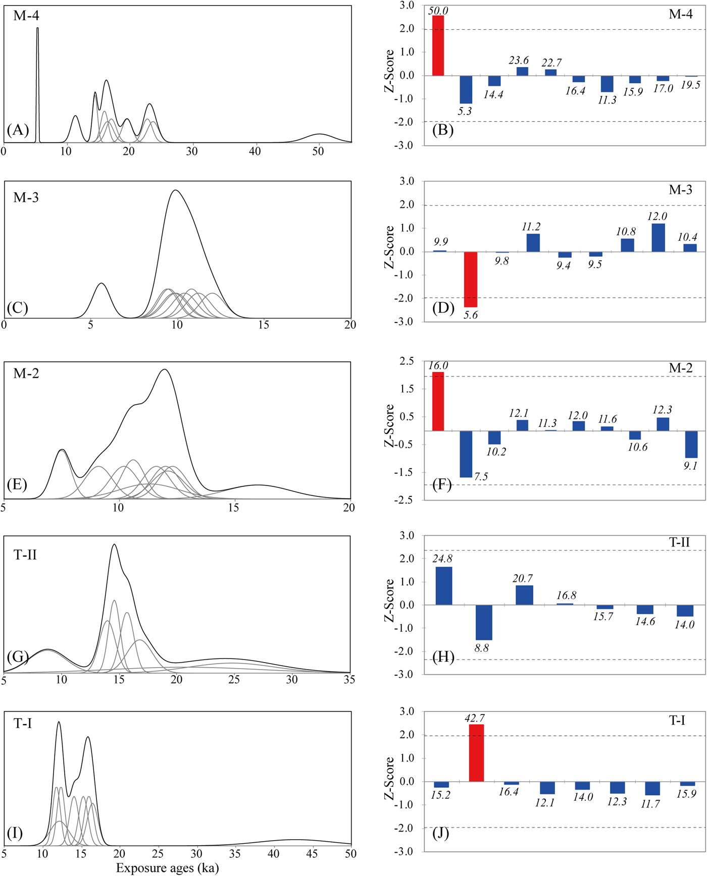
Thirty-four 36Cl exposure ages were obtained from four moraine complexes in the Morrenas Valley. Ten exposure ages from the Chirripó IV moraine (M-4) range from 50.0 ± 2.2 to 5.3 ± 0.1 ka (internal uncertainty). The PDF shows a multimode distribution of ages, and the oldest age of 50.0 ± 2.2 ka and the youngest age of 5.3 ± 0.1 ka are different from the distribution of the other ages from 10 to 25 ka (Fig. 4A). The Grubbs test indicates that the oldest age of 50.0 ± 2.2 ka is an outlier, but not the youngest age of 5.3 ± 0.7 ka (Fig. 4B). The oldest age of 50.0 ± 11.0 ka likely resulted from nuclide inheritance because of prior exposure. The χ R2 value of all these ages is 2341.7 and reduces to 1521.8 after removing the oldest age of 50.0 ± 2.2 ka. As discussed in the “Methods” section, after removing the outlier, we tentatively assigned the oldest age of 23.6 ± 0.9 ka (internal uncertainty) from the remaining ages as the formation age of this moraine because of the high scatter of these ages (χ R2>>1).

Figure 4. (color online) Probability density plots and outlier detection results based on the Grubbs test of 36Cl exposure ages from five moraines in the Morrenas and Talari Valleys. Moraines in the Morrenas Valley include the M-4 moraine (A and B), the M-3 moraine (C and D), and the M-2 moraine (E and F). Moraines in the Talari Valley include the T-II moraine (G and H) and the T-I moraine (I and J). Panels A, C, E, G, and I are the probability density plots, and panels B, D, F, H, and J are the Grubbs test results for outlier detection of these moraines.
Nine exposure ages from the Chirripó III moraine (M-3) range from 12.0 ± 0.7 to 5.6 ± 0.5 ka. The PDF of these ages shows that ages cluster around 10.0 ka (Fig. 4C). The youngest age of 5.6 ± 0.5 ka is detected by the Grubbs test as an outlier (Fig. 4D). The χ R2 value of the remaining ages is 1.65, indicating that these ages were still likely affected by postglacial geomorphic processes. We assigned the oldest age of 12.0 ± 0.7 ka as the age of this moraine.
Ten exposure ages from the Chirripó II moraine (M-2) range from 16.0 ± 1.4 to 7.5 ± 0.4 ka. The PDF of these ages shows that ages cluster around 12.0 ka (Fig. 4E). The Grubbs test indicates that the oldest age of 16.0 ± 1.4 ka is likely an outlier (Fig. 4F). After removing this outlier, the χ R2 value of the remaining ages is 11.4, indicating that these ages were likely affected by postglacial geomorphic processes. We assigned the oldest remaining age of 12.3 ± 0.6 ka as the age of this moraine.
Four exposure ages from the Chirripó I moraine complex (M-1; CS-0, 2, 3, and 4) range from 15.2 ± 1.1 to 9.7 ± 0.5 ka. We did not plot these ages as a PDF because these four samples were collected from separate moraine ridges. We also obtained an exposure age of 20.4 ± 0.4 ka (CS-5) from a higher lateral moraine on the eastern wall of the cirque. It likely corresponds to the older and most extensive Chirripó IV moraine (M-4) down the valley.
Fifteen 36Cl exposure ages were obtained from the two moraines in the Talari Valley. Seven exposure ages from the lower Talari moraine (T-II) range from 24.8 ± 3.7 to 8.8 ± 1.6 ka. The PDF of these ages (Fig. 4G) shows that ages cluster around 14.8 ka; the Grubbs test detects no outliers (Fig. 4H). The χ R2 value of these ages is 9.5, indicating that these ages were likely affected by postglacial moraine degradation. We assigned the oldest age of 24.8 ± 3.7 ka as the age of this moraine.
Eight ages from the upper Talari moraine (T-I) range from 42.7 ± 5.1 to 11.7 ± 0.9 ka. The PDF of these ages (Fig. 4I) shows that ages cluster around 15.8 and 12.0 ka. The Grubbs test indicates that the oldest age of 42.7 ± 5.1 ka is likely an outlier (Fig. 4J), probably because of prior exposure of the boulder (nuclide inheritance). Removing this age from the data set reduces the χ R2 value to 10.1, indicating that the remaining ages were still affected by postglacial degradation processes. We assigned the oldest age of 16.4 ± 0.7 ka as the age of this moraine.
DISCUSSION
Cosmogenic 36Cl exposure ages
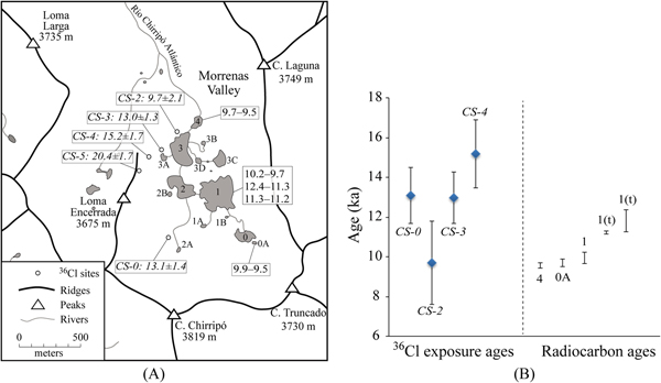
To validate the use of 36Cl surface exposure dating to date glacial landforms in this area, we compared the four 36Cl exposure ages (CS-0, 2, 3, and 4, using external uncertainty) for boulders on moraine ridges in the Chirripó I moraine complex with calibrated radiocarbon ages based on dates on bulk sediment and charcoal in basal sediments of three glacial lakes within the cirque of the Morrenas Valley (Horn, Reference Horn1990; Orvis and Horn, Reference Orvis and Horn2000; Lane et al., Reference Lane, Horn, Mora, Orvis and Finkelstein2011; Fig. 5A). The radiocarbon dates were recalibrated using Calib 7.0.2 (Stuiver and Reimer, Reference Stuiver and Reimer1993) and the data set of Reimer et al. (Reference Reimer, Bard, Bayliss, Beck, Blackwell, Ramsey and Buck2013). Three radiocarbon dates were on material from just above the transition from mineral glacial facies to organic sediment in Lake 4 (AMS 14C on organic sediment; Orvis and Horn, Reference Orvis and Horn2000), Lake 1 (standard 14C analysis on sediment; Horn, Reference Horn1990), and Lake 0A (AMS 14C on charcoal; Orvis and Horn, Reference Orvis and Horn2000). These samples yielded calibrated age ranges (95% confidence, rounded) of 9.7–9.5 ka cal BP for Lake 4, 10.2–9.7 ka cal BP for Lake 1, and 9.9–9.5 ka cal BP for Lake 0A. Horn (Reference Horn1990) also obtained a standard radiocarbon date on transitional sediment (mineral silt with sparse organics) below the basal organics in Lake 1, and Lane et al. (Reference Lane, Horn, Mora, Orvis and Finkelstein2011) obtained an AMS date on a 2 cm section of sediment that spanned the transition from mineral to organic sediment. The calibrated age ranges for these samples are 12.4–11.3 ka cal yr BP and 11.3–11.2 ka cal yr BP, respectively.

Figure 5. (color online) (A) An enlarged lake map marked with measured 36Cl exposure ages (ka, with external uncertainty) and the calibrated radiocarbon age ranges (ka cal BP, 95% confidence) from basal sediments of three glacial lakes within the cirque of the Morrenas Valley. The code for each lake is based on Orvis and Horn (Reference Orvis and Horn2000). (B) The comparison between the 36Cl exposure ages and the calibrated radiocarbon age ranges. The sample ID is marked for each 36Cl age. The lake code where each calibrated radiocarbon age range was dated is also marked (“t” indicates that the radiocarbon sample consisted of or included transitional sediment below the basal organics).
The comparison indicates that the 36Cl exposure ages are similar but as a set slightly older than the calibrated radiocarbon ages (Fig. 5B). These glacial lakes were formed after the retreat of glaciers, so the radiocarbon ages from basal lake sediments are expected to be somewhat younger than the moraine ages. On the other hand, the 36Cl exposure ages are affected by the uncertainties in the production rates. As indicated by Marrero et al. (Reference Marrero, Phillips, Borchers, Lifton, Aumer and Balco2016a), most calibration sites for production rates are from the middle and high latitudes, and the only site from tropical America, Huancané, Peru (13°S), produced high scatter results and was not included in the production rate calibration. Therefore, the production rates in low latitudes still have relatively large uncertainties. Differences of 5–10% in production rates, for example, could change the exposure age by 5–10%. However, even if the true 36Cl production rates are 5–10% higher or lower than the production rates we used in the calculation, the derived 36Cl exposure ages are still in agreement with the minimum-limiting ages on lake sediments. This comparison indicates that our 36Cl exposure ages are reliable and can be used to constrain the glacial chronology in this area.
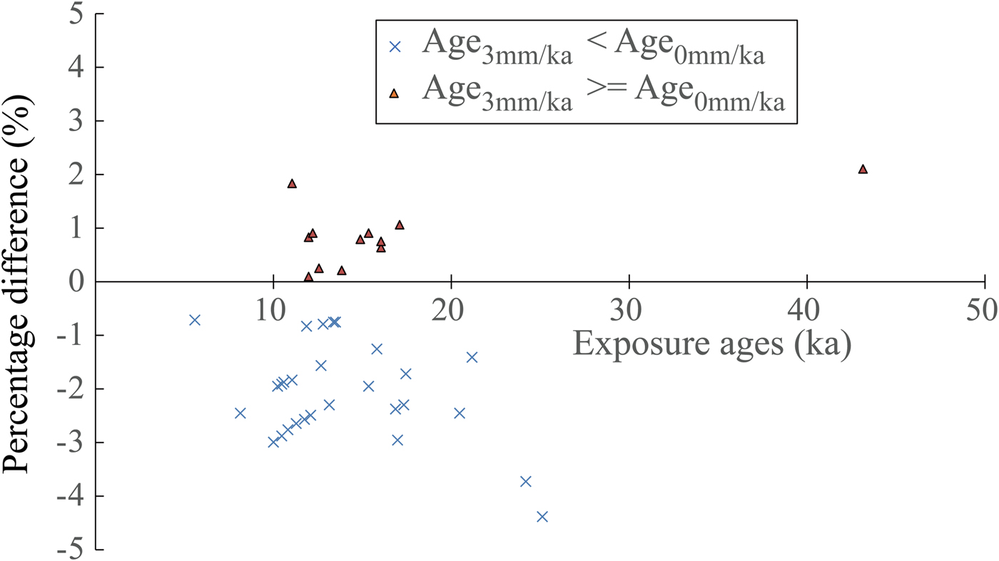
Our calculated exposure ages are based on the assumption of zero erosion of the boulder surface. To examine the effect of boulder surface erosion, we compared our calculated ages with ages derived using a surface erosion rate of 3 mm/ka, a potential maximum surface erosion rate used in many other studies (e.g., Abramowski et al., Reference Abramowski, Bergau, Seebach, Zech, Glaser, Sosin, Kubik and Zech2006; Koppes et al., Reference Koppes, Gillespie, Burke, Thompson and Stone2008; Li et al., Reference Li, Liu, Kong, Harbor, Chen and Caffee2011). Surface erosion does not always result in apparently older 36Cl exposure ages, because of the production of thermal and epithermal neutron reactions. For our samples, the differences in calculated ages derived using these two erosion rates were mainly <5.0% (average 2.0%) (Fig. 6). From this comparison, we conclude that boulder surface erosion does not have a significant impact on the exposure ages in our study. This interpretation is consistent with the sensitivity analysis by Marrero et al. (Reference Marrero, Phillips, Borchers, Lifton, Aumer and Balco2016a) of the impact of different factors on 36Cl exposure age. Based on analyses of calibration data sets, the researchers concluded that erosion rate is a minor contributor (1.0–2.5%) to the uncertainty of 36Cl exposure age (Marrero et al., Reference Marrero, Phillips, Borchers, Lifton, Aumer and Balco2016a). Note that we did not assess the impact of snow cover, as there is no snow in this area in the present climate. We also did not evaluate the influence of moraine degradation, past air pressure conditions, and the water content in the environment on exposure ages (Marrero et al., Reference Marrero, Phillips, Borchers, Lifton, Aumer and Balco2016a), because of the lack of information. Given the apparently minor impact of surface erosion on exposure ages, the wide scatter in the ages does indicate that these moraines were likely affected by postglacial degradation and exhumation. Thus, the use of the oldest age to represent the age of each moraine is reasonable.

Figure 6. (color online) Scatter plot illustrating the difference (%) between the 36Cl exposure ages derived under the assumption of zero surface erosion and using a surface erosion rate of 3 mm/ka.
Glacial chronology in the Chirripó highland
The 36Cl exposure ages show similar timing and extent of glacial events between the Morrenas and Talari Valleys. The exposure ages of the M-4 moraine in the Morrenas Valley are similar to the exposure ages of the T-II moraine in the Talari Valley. The oldest exposure age for the M-4 moraine, which reaches to 3310 m asl, is 23.6 ± 0.9 ka in the Morrenas Valley after excluding one outlier. In the Talari Valley, the oldest exposure age from the T-II moraine (reaches to 3349 m asl) is 24.8 ± 3.7 ka. Similar exposure ages indicate that these moraines of similar extent in two valleys were formed during the same glacial stage, confirming the interpretation of Lachniet and Seltzer (Reference Lachniet and Seltzer2002). Based on our cosmogenic isotope results, we place their formation at 25–23 ka, corresponding to the global last glacial maximum (LGM).
The oldest exposure ages from the M-3 and M-2 moraines in the Morrenas Valley are 12.0 ± 0.7 and 12.3 ± 0.6 ka, respectively. The four 36Cl exposure ages (CS-0, 2, 3, and 4) from the M-1 moraine complex within the cirque of the Morrenas Valley are from 15.2 ± 1.1 to 9.7 ± 0.5 ka with two of these four ages clustering at 13 ka. The close proximity of these moraines (<2 km apart) and their similar exposure ages suggest that they were likely formed during periods of glacial retreats and standstills (15–10 ka) from the deglacial period to Early Holocene. Similarly, the oldest exposure age of the T-I moraine in the Talari Valley is 16.4 ± 0.7 ka after excluding the outlier. This moraine was also likely formed during the deglacial period. The lack of exposure ages younger than ~10 ka within the cirque of the Morrenas Valley is consistent with the interpretation of Orvis and Horn (Reference Orvis and Horn2000), based on radiocarbon dating of lake sediments, that deglaciation of the valley was complete well before 9.7 ka cal BP.
In summary, our exposure ages suggest that all dated moraines within these two valleys were likely formed by glacial advance during the global LGM and periods of glacial retreat and standstill from the deglacial period to Early Holocene. This chronology is much younger than the polystage interpretation of Orvis and Horn (Reference Orvis and Horn2000), who suggested that the Chirripó IV–II moraines in the Morrenas Valley could correspond to MIS 6 to MIS 2. However, our ages fit with the geomorphic interpretation of Wunsch et al. (Reference Wunsch, Calvo, Willscher and Seyfried1999), which attributed the moraines to a single cold stage. Our exposure ages are also consistent with estimates of relative age made by Lachniet and Seltzer (Reference Lachniet and Seltzer2002) using the evidence of the heights of weathered quartz vein pedestals on moraine boulders. Based on relatively small differences in pedestal heights, Lachniet and Seltzer (Reference Lachniet and Seltzer2002) concluded that their Talamanca moraines (M-4 and T-II) were probably no more than a few thousand years older than the Chirripó moraines (M-3 and T-I).
Comparison of glacial chronology with other areas
Our exposure ages indicate that the maximum glacial extent occurred in the Chirripó highland during the global LGM. Many studies have provided evidence of global LGM glacial events in the tropics and subtropics (e.g., Kaplan et al., Reference Kaplan, Coronato, Hulton, Rabassa, Kubik and Freeman2007, Reference Kaplan, Fogwill, Sugden, Hulton, Kubik and Freeman2008; Kull et al., Reference Kull, Imhof, Grosjean, Zech and Veit2008; Bromley et al., Reference Bromley, Schaefer, Winckler, Hall, Todd and Rademaker2009; Hein et al., Reference Hein, Hulton, Dunai, Schnabel, Kaplan, Naylor and Xu2009, Reference Hein, Hulton, Dunai, Sugden, Kaplan and Xu2010; Zech et al., Reference Zech, Zech, Kubik and Veit2009; Glasser et al., Reference Glasser, Jansson, Goodfellow, Angelis, Rodnight and Rood2011; Wesnousky et al., Reference Wesnousky, Aranguren, Rengifo, Owen, Caffee, Murari and Perez2012; Carcaillet et al., Reference Carcaillet, Angel, Carrillo, Audemard and Beck2013). These events were broadly synchronous with the global LGM advances at mid- to high latitudes in North America (Briner et al., Reference Briner, Kaufman, Manley, Finkel and Caffee2005; Briner and Kaufman, Reference Briner and Kaufman2008; Licciardi and Pierce, Reference Licciardi and Pierce2008; Phillips et al., Reference Phillips, Zreda, Plummer, Elmore and Clark2009; Young et al., Reference Young, Briner and Kaufman2009, Reference Young, Briner, Leonard, Licciardi and Lee2011; Rood et al., Reference Rood, Burbank and Finkel2011; Laabs et al., Reference Laabs, Munroe, Best and Caffee2013).
Multiproxy evidence, including isotopic records from ice cores and 10Be exposure ages, indicate broadly synchronous retreat of LGM glaciers in both hemispheres (e.g., Schaefer et al., Reference Schaefer, Denton, Barrell, Ivy-Ochs, Kubik, Andersen, Phillips, Lowell and Schluchter2006; Denton et al., Reference Denton, Anderson, Toggweiler, Edwards, Schaefer and Putnam2010; Putnam et al., Reference Putnam, Schaefer, Denton, Barrell, Birkel, Andersen, Kaplan, Finkel, Schwartz and Doughty2013). Post-LGM warming was punctuated by short cooling phases during the deglacial to Holocene, which likely stalled retreat or caused glaciers to readvance. Exposure ages presented in this study indicate periods of glacial retreats and standstills from the deglacial period to Early Holocene on the Chirripó massif. Previously published chronologies indicated similar events in other tropical and subtropical areas (Vázquez-Selem and Heine, Reference Vázquez-Selem, Heine, Ehlers and Gibbard2004; Farber et al., Reference Farber, Hancock, Finkel and Rodbell2005; Zech et al., Reference Zech, Kull and Veit2006; Pigati et al., Reference Pigati, Zreda, Zweck, Almasi, Elmore and Sharp2008; Bromley et al., Reference Bromley, Schaefer, Winckler, Hall, Todd and Rademaker2009; Hall et al., Reference Hall, Farber, Ramage, Rodbell, Finkel, Smith, Mark and Kassel2009; Smith et al., Reference Smith, Lowell and Caffee2009; Zech et al., Reference Zech, Zech, Kubik and Veit2009; Kaplan et al., Reference Kaplan, Strelin, Schaefer, Denton, Finkel, Schwartz, Putnam, Vandergoes, Goehring and Travis2011; Carcaillet et al., Reference Carcaillet, Angel, Carrillo, Audemard and Beck2013; Jomelli et al., Reference Jomelli, Favier, Vuille, Braucher, Martin, Blard and Colose2014), corresponding to the deglacial to Early Holocene events that have been widely reported in higher latitudes (e.g., Briner et al., Reference Briner, Kaufman, Werner, Caffee, Levy, Manley, Kaplan and Finkel2002; Owen et al., Reference Owen, Finkel, Minnich and Perez2003; Balco et al., Reference Balco, Briner, Finkel, Rayburn, Ridge and Schaefer2009). This study contributes to the growing literature of glacial chronologies in the tropics, strengthening the argument for the broadly synchronous global LGM and deglacial to Early Holocene events between North and South America. In addition, geomorphic evidence, exposure ages, and available radiocarbon dates indicate no glacial events after ~10 ka in either the Morrenas or Talari Valleys. Surface exposure dating of moraines in Venezuela showed similar results, with complete glacial retreat ~9 ka (Carcaillet et al., Reference Carcaillet, Angel, Carrillo, Audemard and Beck2013; Angel et al., Reference Angel, Audemard, Carcaillet, Carrillo, Beck and Audin2016) for a study site at a latitude of ~8°48'N, similar to that of our study area in the Cordillera de Talamanca (9°29'N).
Glacial events have been dated to MIS 3 or older in tropical regions of North and South America. In Mexico, the exposure ages of some old moraines have been dated to ~195 ka (Vázquez-Selem and Heine, Reference Vázquez-Selem, Heine, Ehlers and Gibbard2004). In the Andes, moraines have been dated from MIS 4 to as old, or older than, MIS 13 (Farber et al., Reference Farber, Hancock, Finkel and Rodbell2005; Smith et al., Reference Smith, Seltzer, Farber, Rodbell and Finkel2005, Reference Smith, Mark and Rodbell2008; Kull et al., Reference Kull, Imhof, Grosjean, Zech and Veit2008; Zech et al., Reference Zech, May, Kull, Ilgner, Kubik and Veit2008; Hein et al., Reference Hein, Hulton, Dunai, Schnabel, Kaplan, Naylor and Xu2009, Reference Hein, Hulton, Dunai, Sugden, Kaplan and Xu2010; Glasser et al., Reference Glasser, Jansson, Goodfellow, Angelis, Rodnight and Rood2011). However, our exposure ages do not indicate the occurrence of glacial events before MIS 2 in our study area of the Cordillera de Talamanca. Postglacial geomorphic processes might have eroded the moraines older than MIS 2, or such moraines may be located below the modern treeline and hidden by dense forest cover, especially on the Caribbean side of the massif. It is also possible that glacial events older than MIS 2 occurred in the Morrenas and Talari Valleys but were less extensive than the LGM event, so that the subsequent LGM advance would have overridden these older moraines. Another possibility is that no glacial events occurred in the highland in Costa Rica prior to the LGM. Further studies are necessary to investigate these different possibilities.
Paleoclimate implications
The global LGM is the coldest period during the last glaciation, and studies indicate considerably more cooling in the tropical highlands than at sea level during this period (Crowley, Reference Crowley2000; Lea, Reference Lea2004). The ELA depressions of tropical glaciers during the LGM range from 400 to 1400 m (Porter, Reference Porter2001; Mark et al., Reference Mark, Harrison, Spessa, New, Evans and Helmens2005) with much higher depressions in the circum-Caribbean highlands (Lachniet and Vazquéz-Selem, Reference Lachniet and Vázquez-Selem2005). In our study area of the Cordillera de Talamanca, Costa Rica, reconstructed ELA depressions range from 1317 to 1536 m, indicating a cooling of ~7°C to 9°C during the LGM (Orvis and Horn, Reference Orvis and Horn2000; Lachniet and Seltzer, Reference Lachniet and Seltzer2002; Lachniet and Vazquéz-Selem, Reference Lachniet and Vázquez-Selem2005). Similarly, reconstructed LGM ELAs were ~850 to 1420 m lower than present in the Cordillera de Mérida, Venezuela, suggesting a temperature depression of 8.8 ± 2°C based on a combined energy and mass-balance equation to account for an ELA lowering (Stansell et al., Reference Stansell, Polissar and Abbott2007). Roy and Lachniet (Reference Roy and Lachniet2010) reconstructed ELA depressions during the LGM of 1110 to 1436 m in the Sierra los Cuchumatanes, Guatemala, suggesting a cooling of ~5.9 to 7.6 ± 1.2°C. In contrast, the reconstructions of the sea surface temperatures only indicate 2–3°C depression in the tropics during the LGM (Lee and Slowey, Reference Lee and Slowey1999; Lea et al., Reference Lea, Pak and Spero2000; Pigati et al., Reference Pigati, Zreda, Zweck, Almasi, Elmore and Sharp2008). Several paleotemperature studies from the Cariaco Basin on the north coast of Venezuela indicate a temperature depression of ~3°C to 4°C during the LGM (Lin et al., Reference Lin, Peterson, Overpeck, Trumbore and Murray1997; Lea et al., Reference Lea, Pak, Peterson and Hughen2003).
Various explanations have been proposed to address the discrepancy between the temperature depression reconstructed from the tropical highlands and sea surface during the LGM. One explanation is that the tropical area had a steeper atmospheric lapse rate during the LGM that lowered the freezing height relative to sea surface (Orvis et al, Reference Orvis, Clark, Horn and Kennedy1997; Farerra et al., Reference Farerra, Harrison, Prentice, Ramstein, Guiot, Bartlein and Bonnefille1999; Orvis and Horn, Reference Orvis and Horn2000). Betts and Ridgway (Reference Betts and Ridgway1992) suggested other factors, such as a decrease in surface wind speed or an increase in tropical sea surface pressure, may also lower the freezing height. Roy and Lachniet (Reference Roy and Lachniet2010) proposed that the relatively high ELA depressions in Guatemala may be related to the enhanced wetness driven by southward excursions of the boreal winter polar air mass. More studies are needed in the future to address the discrepancy between the temperature depressions reconstructed from low and high altitudes in the tropics.
After the LGM, the temperature presented an overall warming trend to the Early Holocene, but with significant variability (Thompson et al., Reference Thompson, Mosley-Thompson, Davis, Lin, Henderson, Cole-Dai, Bolzan and Liu1995, Reference Thompson, Davis, Thompson, Sowers, Henderson, Zagorodnov and Lin1998). It seems that the Chirripó III–I (M-3, M-2, and M-1) and the T-I moraines in the Morrenas and Talari Valleys were likely formed during short cooling phases from the deglacial period to Early Holocene.
CONCLUSIONS
We constrained glacial chronology in two formerly glaciated valleys in the Chirripó massif of the Cordillera de Talamanca, Costa Rica, using cosmogenic 36Cl surface exposure dating. Forty-nine boulder samples were processed and measured from four moraine complexes in the Morrenas Valley and two moraines in the Talari Valley. The exposure ages of these samples suggest a major glacial event occurred in this area during 25–23 ka, broadly synchronous with the global LGM, followed by periods of retreats and standstills from the deglacial period to the Early Holocene (16–10 ka). The lack of exposure ages of less than ~10 ka is consistent with evidence from geomorphology and lake sediments that the LGM event and subsequent deglaciation from the deglacial period to the Early Holocene are the most recent glacial events in this area. Cosmogenic exposure ages from these moraines expand the previous glacial chronology determined using radiocarbon ages from basal sediments in glacial lakes and provide important insights into paleoclimate and environmental changes in this tropical highland.
ACKNOWLEDGMENTS
This work was supported by National Science Foundation grant #1227018 to Y. Li and S.P. Horn. Additional support for laboratory analyses and fieldwork was provided by the PRIME Lab (Purdue University), the University of Tennessee, and grants to K.H. Orvis from the American Association of Geographers and to S.P. Horn from the National Geographic Society and the A.W. Mellon Foundation. We thank the Costa Rican Ministry of Environment and Energy and the La Amistad-Pácífico Conservation Area for allowing us to collect samples in Chirripó National Park; Brandon League, Charles Lafon, Carol Harden, and Jose Luis Garita Romero for field assistance; and Maureen Sánchez for logistical assistance. We also thank Chris Fedo, Dakota Anderson, and Yanan Li for laboratory assistance and Marc Caffee, J. Radler, and Tom Clifton for sample preparation and measurement at the PRIME Lab. For constructive comments and suggestions that strengthened the manuscript, we thank Fred Phillips, Lewis Owen, Kathleen Johnson, and an anonymous reviewer.
SUPPLEMENTARY MATERIAL
The supplementary material for this article can be found at https://doi.org/10.1017/qua.2018.133.