


1. Introduction
Genomic information plays only an indirect role in organizing the spatial and temporal order in cells and organisms. Cellular functions – the decisions to grow and divide, to die by programmed cell death, or to stay static – ultimately lie with macromolecules encoded by DNA. Both proteins and RNA directly control the cell through the reactions they perform, the conformations they adopt, and the interactions that they make in solution. A modern, mechanistic understanding of cells, therefore, requires detailed knowledge of the three-dimensional configuration of the atoms involved in these processes.
Macromolecules are inherently near-sighted. Stable macromolecular interfaces involve forces that typically are only effective in short ranges that can be measured in Ångstroms, and these interfaces typically fit together like pieces of a jigsaw puzzle that exclude bulk solvent and leave very few gaps at the shared surface. Conformational changes, driven by small-molecule binding, allostery, or complex formation can be propagated through long distances. But even these changes are only the sum of short-range interactions between atoms. Ultimately, even the integration of these macromolecules and macromolecular complexes into pathways requires an appropriate milieu in which the macromolecules can act and be acted on. Macromolecules can be thought of as ‘cogs in the machine’ in which pathways and networks are the result of the availability of substrates.
Cellular coordination, in which macromolecules serve as bit players, functions as a gestalt, where the whole is greater than the sum of its parts. Macromolecules are controlled through their creation and their destruction and through reversible modifications, such as phosphorylation, methylation, and ubiquitination. Functional modification and even control of synthesis and degradation are mechanisms requiring the formation of dynamic interfaces and conformational states that control the macromolecule either directly, through activation or inactivation of the macromolecule of interest, or indirectly through pathways that affect the macromolecule. At its core, each of these levels of control is expressed through the shapes of specific macromolecules. Control of shape is control of information. Thus it seems highly appropriate that the English word ‘information’ is derived from the Latin informare, meaning to ‘form’, ‘shape’, or ‘organize’.
We believe that the major challenge for structural biology in the next decade will be in providing a mechanistic understanding of the macromolecular and supramolecular complexes and their conformational changes that underlie cell biology and in using these structures to provide new opportunities in the medical, biotechnological, and pharmaceutical fields. Addressing these challenges is fundamentally important from a scientific standpoint, yet tremendously difficult from a practical one. Our experience has suggested that many of the most important problems will involve macromolecular complexes whose structures and complexes will not be easily solved by any single biophysical technique. Thus advances will require the use and development of methods to bridge atomic resolution structures determined by X-ray crystallography and NMR with lower resolution information about large complexes and conformational states that are too flexible, too large, or too difficult to stabilize as homogeneous samples for these techniques. Recent substantial investments in NMR spectrometers and synchrotron facilities combined with impressive advances in electron microscopy (EM) and cryo-tomography of very large complexes has led to important advances in understanding important macromolecular complexes (Dubochet et al. Reference Dubochet, Adrian, Chang, Homo, Lepault, McDowall and Schultz1988; Lucic et al. Reference Lucic, Forster and Baumeister2005; Craig et al. Reference Craig, Volkmann, Arvai, Pique, Yeager, Egelman and Tainer2006; Scheres et al. Reference Scheres, H. Valle, Herman, Eggermont, Frank and Carazo2007). We predict, however, that the combination of X-ray crystallography and small-angle X-ray scattering (SAXS) is well poised to become an important technique for generating structures in solution with a resolution range from roughly 50 Å to 10 Å. Both techniques are becoming increasingly accessible to a broad range of investigators. Sample preparation for SAXS analysis is particularly accessible to a variety of laboratories which otherwise may have thus far never used structural techniques.
As a solution technique, SAXS offers the potential for obtaining some information with every sample, requires modest sample preparation and material relative to crystallography, and is a natural technique for understanding systems possessing substantial flexibility. SAXS can characterize shape and conformation in solution for quite small to very large macromolecular systems, spanning the ranges limiting NMR and EM methods. The combination of current third-generation synchrotron sources and sophisticated computational techniques has substantially increased the utility of SAXS. Experiments can be performed much more rapidly than either EM or crystallographic experiments. In addition, information derived from SAXS data can be useful both prior to and after high-resolution structures are solved. The information content in scattering curves is substantially less than that in crystallography, which is an inherent limitation of this technique. However, SAXS data can be used to determine the low-resolution structures of macromolecules without any additional experimental information. Moreover, SAXS is not only likely to be more powerful in conjunction with atomic resolution structures to provide more accurate and complete models of protein, RNA, and DNA structures, conformations, interactions, and assemblies in solution. The accessible experimental resolution can thus be made appropriate to the biological question being asked. SAXS measurements can directly define the global shape and conformation in solution, whereas the combination of SAXS with computation plus high-resolution component structures provides more detailed three-dimensional information. We therefore expect that SAXS will return any investments made into development of experimental resources or additional computational techniques.
This review aims to provide a general framework for making informed decisions about experimental design, data processing, and data interpretation to combine SAXS with atomic-resolution structures from crystallography through computational methods. For the purpose of bringing everyone to the same level, Section 2 provides a comparative assessment of X-ray diffraction and scattering techniques. Section 3 considers computational techniques for modeling macromolecular flexibility, which are important for understanding most of the methods used for fitting and deforming atomic structures in the context of low-resolution information. Section 4 focuses on the principal means to directly compare SAXS data and crystal structures, employ SAXS experiments to derive ab-initio SAXS models, and appropriately consider flexibility and disorder in SAXS experiments. Section 5 details specific experimental strategies and tactics and provides a basis to assess the value of different interpretations of SAXS data for a given experiment. Section 6 outlines our views on the prospects for further developments and applications of SAXS to define experimentally validated macromolecular shapes and conformations in solution and provide more complete information than can be typically obtained by either technique alone. At the same time we note concerns and areas where we believe SAXS in particular will benefit from a directed research effort. An overall goal of this review is to provide the framework for improved collaborative efforts involving SAXS with other techniques with the belief that problem-driven developments will help push substantial improvements in SAXS technologies and software with obvious and important relevance to the understanding, simulation, and prediction of macromolecular interactions and conformations in solution.
2. Comparison of crystallography and SAXS techniques
SAXS and X-ray crystallography are fundamentally similar techniques and can share most of the hardware required to generate, prepare, and detect X-rays. In most experiments, a collimated, monochromatic beam of X-rays irradiates a sample, and the intensities of the scattered (SAXS) or diffracted (crystallography) X-rays are measured by an X-ray detector (Fig. 1a).

Fig. 1. X-ray interactions with sample for SAXS and crystallography. (a) Both SAXS and X-ray crystallography involve placing a sample (orange) into a highly collimated X-ray beam (red) and measuring the scattered X-rays. The angle of any scattered position with the direct beam is 2θ. (b) Scattering from a solution of yeast PCNA with a maximum resolution of 23·9 Å. (c) Diffraction from a nickel superoxide dismutase crystal at 2·0 Å resolution. The equivalent position of the highest resolution of the SAXS experiment is indicated (red circle). The blue circle indicates the highest resolution achievable (q=0·6 Å−1) for SAXS data collection at SIBYLS. Both images collected at beamline 12.3.1 (SIBYLS) at the Lawrence Berkeley National Laboratories. Diffraction image courtesy David Barondeau, Department of Chemistry, Texas A&M University.
A fundamental difference between solution scattering and X-ray crystallography lies in the relative organization of target molecules during data collection. In solution scattering, the signal from all orientations of the target molecules, relative to one another and the experimental apparatus, are averaged together. Solution scattering is continuous and radially symmetric (isotropic) (Fig. 1b, c). In contrast, in X-ray crystallography the molecules are highly organized within a crystal lattice. Diffraction from a crystal lattice gives rise to discrete diffraction maxima that are caused by the convolution of the crystal lattice onto the continuous transform due to the atomic positions and provides enormously greater signal. Moreover, the lack of radial symmetry in crystallography retains information about specific orientations in the molecule and requires that crystals be rotated during data collection (Dauter, Reference Dauter1997). Crystallography provides substantially more information content than SAXS, allowing atomic resolution structures to be determined; however, the requirement of packing in the crystal lattice can lead to molecules whose conformations are inappropriately fixed by non-biologically relevant interactions (Section 4.2.4).
The theoretical underpinnings for both of these techniques are well understood and have been the subject of recent reviews (Koch et al. Reference Koch, Vachette and Svergun2003) and excellent books (Blundell & Johnson, Reference Blundell and Johnson1976; Giacovazzo et al. Reference Giacovazzo, Monaco, Viterbo, Scordari, Gilli, Zanotti and Catti1992; Drenth, Reference Drenth1994). Our goal here is therefore to not to exhaustively address each technique, but to introduce and draw parallels between them. We expect that crystallographers will benefit primarily from the introduction to SAXS and that SAXS specialists will benefit most from the introduction to macromolecular crystallography. We highlight areas of overlap with the expectation that some appreciation of both techniques will be important for using these paired X-ray techniques for the growing number of multi-resolution structure-determination problems.
2.1 Interactions of X-rays with matter
Both SAXS and X-ray crystallography exploit coherent (Thomson) X-ray scattering. In coherent scattering, electrons oscillating under the influence of the electric field of the X-ray beam act as secondary sources, emitting X-rays with the same wavelength as the incident beam, but 180° out of phase. The scattering measured at an angle of 2θ relative to the direct beam is proportional to (1+cos2 2θ), reaching a maximum when the scattering is parallel to the incident X-ray beam (2θ=0°) and falling off at large 2θ angles. Atomic scattering factors have been accurately calculated for all of the elements and are influenced by the number of electrons for the atom and the orbitals the electrons occupy. In general, the intensity of coherently scattered X-rays decreases with increasing X-ray energies (decreasing X-ray wavelength). This decrease is discontinuous at energies near atomic orbital-binding energies unique to each atom. The atomic-scattering factors at these energies are described by additional terms accounting for this behavior. Use of this ‘anomalous scattering’ has become an important method for solving protein crystal structures (Section 2.2.5).
The theoretical limit for the resolution, the minimum distance (d min) at which two objects can be distinguished, is based on the wave properties of the X-rays:
where λ is the X-ray wavelength. In practice, the wavelengths typically chosen at synchrotron radiation sources (0·8–1·5 Å) are selected to limit damage to the crystal or to take advantage of anomalous scattering. The theoretical d min values of these wavelengths are typically much smaller than can be measured (typically 3 Å to 1 Å) from crystals of macromolecules due to internal disorder or size of the crystal, and are significantly smaller that those that can be meaningfully recorded in SAXS experiments (typically 50 Å to 10 Å, depending on the sample).
Neutrons can also be used in both crystallographic (neutron diffraction) and solution (small-angle neutron scattering; SANS) experiments (Gutberlet et al. Reference Gutberlet, Heinemann and Steiner2001). Neutrons differ, however, in the fact that they interact with atomic nuclei and thus generate substantially fewer radicals than X-rays during the experiment. Radical formation is known to reduce redox-active sites, such as disulfides and metal centers, and increase sensitivity of biological samples to X-rays (Burmeister, Reference Burmeister2000; Ravelli & McSweeney, Reference Ravelli and McSweeney2000). Unfortunately, the recent increases in X-ray source intensities has not been mirrored by the fission reactors or spallation sources that currently generate thermal neutrons (Taylor et al. Reference Taylor, Dunne, Bennington, Ansell, Gardner, Norreys, Broome, Findlay and Nelmes2007). Signal-to-noise problems with neutron diffraction and scattering experiments are significant challenges to obtaining high-quality data sets. Such neutron experiments involve more specialized efforts and have been well discussed in detail elsewhere (Gutberlet et al. Reference Gutberlet, Heinemann and Steiner2001). Herein we consider X-ray-based experiments, which have broader general utility and applicability to macromolecular systems.
2.2 X-ray crystallography
2.2.1 Crystal lattices – unit cells – symmetry
X-ray crystallography requires the generation of crystals, and macromolecular crystals are typically grown under conditions where molecules are reversibly driven out of solution (Weber, Reference Weber1997). Macromolecular samples require that these conditions are gentle and do not cause unfolding or disassociation of complexes. Typically, crystal lattice forces are much weaker than macromolecular folding energies.
Crystals are ordered arrays of atoms related by pure translation (a transformation with only a change in position but not orientation or rotation) in one dimension (fibers), two dimensions (sheets), and three dimensions (lattices). Although fiber diffraction of samples such as DNA can be studied with X-rays, the most common crystals studied by macromolecular crystallography are three-dimensional. The smallest repeating unit of the crystal that is related only by translations is called the unit cell. For three-dimensional crystals, the shape and size of the unit cell is defined by the length of three axes (a, b, and c) and three angles between these axes (α, β, and γ).
Frequently, internal symmetry exists within the unit cell when the unit cell contains multiple molecules. If these symmetries apply to the entire lattice, they are crystallographic symmetries and constrain the parameters of the unit cell. The smallest portion of structural information required to reconstruct the entire lattice through crystallographic symmetries and lattice translations is termed the asymmetric unit. In contrast, symmetries that do not apply to the lattice are non-crystallographic.
In many cases the biologically relevant complex possesses symmetry. These biological symmetries may be observed by some combination of both the crystallographic and non-crystallographic symmetry operators, if the appropriate assembly is present in the crystal structure. For crystallographic analysis, non-crystallographic symmetries can be tremendously useful for map improvement (Section 2.2.6), as well as generation of constraints for the refinement of atomic models, such as have been implemented in the program CNS (Brunger et al. Reference Brunger, Adams, Clore, DeLano, Gros, Grosse-Kuntsleve, Jiang, Kuszewski, Nilges, Pannu, Read, Rice, Simonson and Warren1998). Analogously, particle symmetry provides important constraints on model-based and ab-initio reconstruction of three-dimensional shapes from one-dimensional SAXS data (Sections 4.2 and 4.3). Application of these symmetry constraints, like use of the non-crystallographic symmetries in crystallography, substantially increases the accuracy of the final models.
2.2.2 Diffraction from crystals and Laue conditions
X-rays diffracted from crystals can be mathematically treated as if they were being reflected from a plane of angle θ to the incident X-rays, and hence the diffraction maxima measured during the crystallographic experiment are frequently termed ‘reflections’. By this definition and due to the geometry of the diffraction event, the diffracted X-rays make an angle of 2θ with incident beam, and thus 2θ is the experimentally measured angle between the direct beam position and the diffraction maximum on the X-ray detector (Fig. 1a).
As electromagnetic waves, X-rays possess both a wavelength and phase. In the crystal, X-rays are diffracted from multiple parallel planes simultaneously, and this leads to a path difference through which these X-rays travel. When the path difference corresponds to an integral number of wavelengths of the incident X-ray, then the diffracted X-rays undergo constructive (in-phase) interference and can be detected experimentally as diffraction maxima. If not, then the X-rays interfere destructively (out-of-phase) and are not observed. This requirement can be expressed mathematically using the Laue conditions:
where a, b, and c are vectors corresponding to the orientation of the unit cell edges, S is the vector corresponding to the path difference between incident and scattered X-rays, and h, k, and l must be integers to ensure constructive interference. The h, k, and l values are the Miller indices and are used to identify each reflection. Thus, the planes that scatter X-rays are determined by the wavelength of the incident X-rays (or wavelengths in the case of Laue multi-wavelength diffraction experiments), the unit cell parameters, and the orientation of the crystal. The Laue conditions give rise to a regularized lattice of diffraction spots (Fig. 1c). Importantly, the unit cell size, shape, and orientation, but not the positions of atoms in the unit cell, control which reflections are in the diffraction condition and where these diffracted reflections occur on the detector. This allows crystallographers to collect, index, and process diffraction data prior to knowing the atomic structure.
Bragg's law provides a measure of the distance between the theoretical planes giving rise to X-ray scattering:
By analogy to light scattering through slits, in the case of a theoretical perfect crystal of infinite size the first-order spectrum will occur when n=1, a second-order spectrum will occur at n=2, and so forth. The maximum resolution (smallest spacing between planes) measured from the crystal can provide insights into its suitability for data collection and structure determination. In contrast, evaluating samples in SAXS for suitability for structural reconstruction is more difficult because every macromolecular solution will scatter X-rays. In this sense, determining if a SAXS curve is suitable for further analysis (Section 5) is more reminiscent of determining if a crystal is merohedrally or pseudo-merohedrally twined (Yeats, Reference Yeats1997), rather than whether or not it can diffract X-rays.
2.2.3 Intensities and atomic arrangements
In contrast to the positions of the reflections, the intensities of the diffracted X-rays are dictated by the atomic arrangements in the unit cell. The positions and types of atoms within the unit cell control both the amplitude and phase. Mathematically,
where F(h, k, l) is the structure factor, h, k, l are the Miller indices of the structure factor, f j is the resolution-dependent atomic scattering factor, and x j, y j, and z j are the fractional positions of the jth atom in the unit cell. Unfortunately, data collection only allows measurement of the intensities, I(h, k, l), which are the square of the amplitude of F(h, k, l), but not the relative phase information necessary to calculate the electronic distribution in the unit cell. Measurement of the relative phase of X-rays striking the detector at any two diffraction spots has not been possible. This problem is the ‘phase problem’ of protein crystallography that must be solved in order for structures to be determined.
In general, measured intensities are on a relative scale, not an absolute one. From a theoretical standpoint, I(0, 0, 0) is the square of the sum of the number of electrons in the unit cell and is directly comparable to the important SAXS result where I(0) is proportional to the square of the number of electrons in the scattering particle (Section 2.3.2). Data in crystallography are generally put on only a quasi-absolute scale using the Wilson plot (Wilson, Reference Wilson1942) using data between 3·0 Å and 1·5 Å resolution. Placing the data on a true absolute scale is, however, quite difficult. In addition to the ordered atoms, the non-ordered bulk solvent must be included in the calculation, which can be demonstrated by the importance of modeling bulk solvent in refining X-ray structures against low-resolution reflections (Urzhumtsev & Podjarny, Reference Urzhumtsev and Podjarny1995). In contrast, the contribution of bulk solvent is explicitly subtracted out during SAXS data processing and typically is involved in the modeling process as a scale factor between calculated and observed intensities. This subtraction is the basis of contrast variation techniques where matching the average electron density of bulk solvent to specific components of a scattering complex causes their contributions to be eliminated from the processed SAXS data (Section 2.3.6).
The crystal lattice has two effects. First, the orientation of the molecules allows the diffraction data to retain information about atomic positions in three-dimensional space, which is lost in SAXS data collected on molecules in solution that are orientationally averaged. Second, the scattering from the atoms in the unit cell is convoluted with the scattering from the lattice so that the crystal diffraction is sampled only at discrete positions defined by unit cell, which also increases signal-to-noise. The measured X-ray intensities in crystallography are the square of the summed amplitudes from the atoms in the unit cell. In contrast, SAXS intensities are the sum of the squared amplitudes from each scattering event. SAXS data are also continuous and vastly over-sampled in comparison to the independent data content as derived from Shannon's theorem. Even with higher signal-to-noise, crystallographic data are substantially under-sampled and cannot take advantage of ‘super-resolution’ techniques that rely upon over-sampling to determine the phases of measured reflections (Koch et al. Reference Koch, Vachette and Svergun2003). Hence, techniques to solve the phase problem use additional information (Section 2.2.5).
2.2.4 The Patterson function
The autocorrelation function for the electron density, which is essentially a three-dimensional map of all of the atom–atom vectors in the crystal, can be written as:
where u, v, w correspond to some difference vector between the position x, y, and z and x+u, y+v, and z+w. Thus N peaks in the electron density map (atoms) will give rise to N 2 peaks in the Patterson function. It has been shown that the above formulation is equivalent to the expression:
where F(h, k, l) is the observed amplitude and V is the volume of the unit cell. The importance of the second expression is that this function can be calculated in the absence of any phasing information, and this function is important for several macromolecular phasing techniques (Section 2.2.5).
When the Patterson function is calculated using the measured amplitudes F(h, k, l), the largest peaks in the autocorrelation are the positions of direct translations between molecules in the crystal lattice; this Patterson function is typically called the ‘self-Patterson’ (Fig. 2). The self-Patterson function in crystallography is an autocorrelation function and is related to the autocorrelation function, P(r), calculated from the SAXS intensities (Section 2.3.3). Unlike the SAXS P(r) function, the crystallographic Patterson function is calculated from molecules that are restricted in their rotations and thus retains three-dimensional information about the inter-atomic vectors (Fig. 2). Additionally, the Patterson function includes all vectors between atoms for all molecules within the crystal. The P(r) function, on the other hand, is a histogram of distances that are orientationally averaged and correspond only to the scattering particle.

Fig. 2. Comparison of the Patterson autocorrelation function in X-ray crystallography and the pair-distribution autocorrelation function in SAXS. A theoretical two-dimensional molecule of four atoms is placed in an arbitrary two-dimensional crystal in solution. The Patterson function contains cross peaks for every interatomic distance in the crystal and these cross-peaks in the u,v-plane, are indicated by circles and retain directional information about their positions in the crystal. The cross-peaks between symmetry mates are not shown in the expanded view due to the size of the unit cell. The pair-distribution function, on the other hand, resolves distances but not directions within each scattering unit. Thus, all equivalent distances in the four-atom molecule add together.
2.2.5 Phase determination
To build a map of the electron density in the unit cell by adding together the diffracted X-ray waves, it is necessary to determine phases for each of the reflections whose intensity is measured. The phases of reflections are not constrained mathematically unless they possess special symmetry relationships. The phase for each reflection needs to be determined and one of three techniques is used: experimental methods, direct methods, and molecular replacement.
Experimental phasing techniques systematically perturb the intensities in ways that can be used to extract information about the relative phases of the measured reflections. Isomorphous replacement (IR) depends upon the introduction of ‘heavy atoms’, e.g. atoms with a large number of electrons such as mercury or uranium, into crystals without perturbing the overall lattice (Ke, Reference Ke1997). To take advantage of the heavy atoms for phasing information, the positions of these atoms must first be identified either through analysis of Patterson maps calculated from differences in intensity or through direct methods (as described below). For determining heavy atom positions, the differences in the amplitudes between the heavy atom derivative and the native crystal are used. From the N 2 peaks in the u, v, w space of the Patterson function and the symmetry of the crystal, the N peaks in x, y, z space can be calculated. Importantly, as the number of sites where the heavy atom binds increase, so do the number of Patterson peaks. Thus Patterson-based methods for solving heavy atom positions can quickly become challenging to solve. Moreover, as the size of the unit cell increases, the height of each Patterson peak becomes relatively weaker; for particularly large unit cells, heavy atom clusters, such as Ta6Br122+, are used instead of single heavy atoms (Knablein et al. Reference Knablein, Neuefeind, Schneider, Bergner, Messerschmidt, Lowe, Steipe and Huber1997).
The other major experimental phasing technique relies upon introducing atoms with anomalous scattering or dispersion into the crystal. Anomalous scattering occurs when X-ray energies are near electronic (typically) or nuclear excitations and are typically described as:
where f is the scattering factor of the atom, f 0 is the wavelength-independent component of the scattering, and f′ and f″ are the real and imaginary parts of the atomic scattering. At any wavelength, f′ is constant, so that f′ differences can only be measured by comparing data at different wavelengths. The imaginary part, the photoelectric absorption f″ (Fig. 3a), however, leads to a breakdown in Friedel's law so that the amplitude of the Friedel pairs [F(h, k, l) and F(−h, −k, −l) are not the same. Phasing experiments that use multiple wavelengths, and can take advantage of both f′ and f″ differences (multi-wavelength anomalous dispersion, MAD) or at a single wavelength that can only use f″ differences (single-wavelength anomalous dispersion, SAD) can be performed. Both SAD and MAD experiments use wavelengths at the atomic transitions to maximize the information. Further, experiments using f″ differences must have carefully measured Friedel pairs. As for MIR, the positions of anomalous scatters can also be determined by Patterson-based techniques (Fig. 3b; Hendrickson & Ogata, Reference Hendrickson and Ogata1997) and used to determine phases (Fig. 3c, d). Because phase information can be readily combined, it is not unusual for the anomalous signal from heavy atom derivatives (MIRAS) to be used and potentially combined with phasing information from other sources such as MAD or SAD experiments or even partial structures (Blow & Crick, Reference Blow and Crick1959; Sim, Reference Sim1959). Anomalous dispersion techniques have become a method of choice for solving crystal structures due to the tunability of synchrotron radiation (Helliwell, Reference Helliwell1997), the ability to cryo-cool and collect datasets from single crystals (Hope, Reference Hope1990; Garman & Schneider, Reference Garman and Schneider1997), and the techniques to introduce anomalous scatters such as selenomethionine in proteins and bromouridine in DNA molecules (Doublie, Reference Doublie1997). Anomalous scattering has also been used in conjunction with SAXS (ASAXS) (Stuhrmann, Reference Stuhrmann1981; Miake-Lye et al. Reference Miake-Lye, Doniach and Hodgson1983); however, the orientational averaging of SAXS data eliminates the f″ component, so that anomalous differences can only be measured between wavelengths. In theory, ASAXS has a number of potential applications such as monitoring the distance between two anomalous scatters; however, the signal is small and most applications have involved simple biological systems such as ion solvation of DNA (Andresen et al. Reference Andresen, Das, Park, Smith, Kwok, Lamb, Kirkland, Herschlag, Finkelstein and Pollack2004), and anomalous scattering is not yet as important in SAXS as it is in macromolecular crystallography.

Fig. 3. The structure of E. coli YgbM determined by selenomethionine MAD. (a) Comparison of theoretical and measured X-ray fluorescence at the selenium edge for the crystal. (b) Anomalous difference Patterson map identifying the selenomethionine Met11-Met11 and Met105-Met105 cross-peaks generated by crystallographic symmetry operators (at the Harker section) calculated using differences between Friedel pairs at the selenium fluorescence inflection point (panel a). (c) Anomalous difference density contoured at 5σ above the mean superimposed with the final refined structure. (d) 2F o−F c experimental electron density after MAD phasing and density modification contoured at 1σ (green), 3σ (lime), and 5σ (yellow). (e) Final refined structure and 2F o−F c map calculated using final refined phases at 1σ (blue), 3σ (orchid), and 5σ (red). (f) Overall structure of YgbM, a zinc-containing TIM-barrel, is shown as a cartoon.
Direct methods, on the other hand, have been primarily used in macromolecular crystallography as an alternative to Patterson-based methods for solving heavy-atom or anomalous-scattering substructures (Weeks et al. Reference Weeks, Blessing, Miller, Mungee, Potter, Rappleye, Smith, Xu and Furey2002). Direct methods take advantages of relationships between phases between multiple reflections (Giacovazzo et al. Reference Giacovazzo, Monaco, Viterbo, Scordari, Gilli, Zanotti and Catti1992) and require that data are complete, accurate, and are of high enough resolution so that individual scatterers can be resolved (resolutions of better than 1·2 Å). In macromolecular crystallography, direct methods can be readily applied to substructure determination, as atoms in these substructures typically are much more than 1·2 Å apart and fit the ‘atomaticity’ requirements even at moderate resolutions. Direct methods have been able to determine large anomalous substructures (Weeks et al. Reference Weeks, Blessing, Miller, Mungee, Potter, Rappleye, Smith, Xu and Furey2002), despite the fact that the use of the differences between intensities rather than intensities introduces some noise into the substructure determination. The determination of these substructures will likely continue to be one of the major roles for this technique in macromolecular crystallography.
Unlike the other techniques described above, molecular replacement attempts to computationally position an atomic model using experimental intensities. From the positioned molecule or molecules, phases can then be calculated for the calculation of electron density maps. The atomic model must be ‘similar’ to the structure of the crystallized molecule, where the degree of similarity depends on the number of molecules to be found and any potential conformational changes that can occur. Molecular replacement is a six-dimensional search; however, proper rotation of a model will allow a calculated Patterson function containing all interatomic vectors to correlate well with one calculated from the experimental data. This allows the problem to be broken down into a three-dimensional rotational search, followed by a three-dimensional translational search. In the rotation search, typically only vectors within a radius similar to the longest intramolecular distance are considered; however, the close intermolecular vectors between atoms in the atomic packing and non-crystallographically related molecules with other orientations result in ‘noise’ in this search. Increasing the number of molecules in the asymmetric unit typically makes the molecular replacement problem more difficult. Similarly, the translation function can also be calculated by comparing the Patterson function from the experimental data with the Patterson functions calculated from rotated molecules to which different translations have been applied. Although molecular replacement can be performed by calculating and overlaying explicitly calculated Patterson functions, faster algorithms that do the equivalent searches are used in practice (e.g. Navaza, Reference Navaza2001).
Molecular replacement solutions introduce the possibility of model-biased phases, which generate maps that do not show the differences between the atomic model used to solve the structure and the electron density that gives rise to the scattering. Importantly, model bias tends to increase as homology with the atomic model decreases, but can be detected through the use of omit maps, which are calculated with portions of the model omitted in the phase calculation. For true solutions, the electron density for the omitted regions will still be observed. For phase-biased results that are entirely dependent upon the model, no electron density will be observed in these omitted regions. As the number of solved protein structures increases, the ability to use molecular replacement to rapidly screen through all reasonable or all possible molecular replacement targets will increasingly become a reasonable strategy to solve new structures. To this end, the ability to identify overall structural similarities through comparison of experimental and calculated SAXS (see Section 2.4.3) could greatly reduce the number of atomic models to be screened and thereby improve the efficiency and success of molecular replacement methods for crystallography.
2.2.6 Structure determination
Given an initial set of phases, either from experimental or computational sources, electron density maps of the unit cell can be calculated. Frequently initial phase information has substantial errors; however, the goal is to generate a map of sufficiently good quality so that an atomic model can be built. Multiple density modification techniques can be used to improve phase information. The two most important ones are solvent flattening or flipping and non-crystallographic symmetry averaging (Vellieux & Read, Reference Vellieux and Read1997; Zhang et al. Reference Zhang, Cowtan and Main1997). These density modification techniques mainly operate by directly modifying the electron density maps and back calculating new phases. Solvent flattening and solvent flipping operate on the assumption that the bulk solvent regions in crystals should have uniform density and that both positive and negative deviations should either be flattened to this average density or flipped in magnitude. Non-crystallographic symmetry averaging, on the other hand, averages the density between non-crystallographically related molecules. Use of these phase modification techniques not only allows for the improvement of initial phases, but also allows for phase extension in cases where experimental phasing information is at lower resolution than the native dataset (Fig. 3d).
From the initial interpretable maps, an atomic structure is usually fit through rounds of atom placement followed by automated refinement (Kleywegt & Jones, Reference Kleywegt and Jones1997). Although experimental maps after phase modification techniques can be of excellent quality, it is possible to place atoms into maps that retain substantial errors in the phases. Thus it is quite common, although not required, to use maps calculated from phases from the updated model itself (Fig. 3e). In the case of atomic partial models or excellent experimental phases, the phases calculated from the model itself can also be combined with experimental phasing information. The crystallographers normally evaluate the experimental electron density map, calculated with the Fourier coefficients 2F o−F c, and the difference electron density map, calculated with the coefficients F o−F c, where F o(h, k, l) are observed amplitudes and F c(h, k, l) are calculated amplitudes. Placement of residues into maps can now be automated, such as by the program suite ARP/wARP (Perrakis et al. Reference Perrakis, Morris and Lamzin1999) and RESOLVE (Terwilliger, Reference Terwilliger2003), which can allow for rapid building of macromolecular structures by cycling between an automated density modeling and model refinement programs, given initial phases with sufficient quality. In these cases, the crystallographer supervises the process and corrects regions that are wrong or are trapped by refinement into local minima.
The overall agreement of the model of the asymmetric unit with the experimental data is measured by the ‘R-factor’:
where F o(h, k, l) are observed amplitudes and F c(h, k, l) are amplitudes calculated from the model. This number allows the crystallographer to monitor the effects of making manual modifications to the structure as well as providing a numerical target for minimization by automated refinement packages.
One important advance in helping detect the problem of overfitting is the R free parameter, which calculates an R-factor for the current model using a set of reflections, typically several thousand, that are withheld from the refinement calculation (Brunger, Reference Brunger1992). However, R free is a global parameter and while it can help determine overfitting, it is not sensitive enough to evaluate the validity of small changes to the crystallographic model. Moreover, choosing the number of reflections and which reflections to include in an R free set can be difficult, particularly when substantial non-crystallographic symmetry exists. Although R free is imperfect in some ways, it is a universally accepted measure of quality which is useful for both crystallographers and external reviewers. In contrast to X-ray crystallography, an appropriate analog to the R-factor is under debate (Section 4.1), and there currently is no suitable SAXS analog to R free (Section 6).
2.2.7 Structure refinement
Crystallographers are aware that molecules in crystals are not completely rigid and are composed of atoms held together by electrons in specific orbitals. However, crystallographers are constrained in their ability to fit these features by the amount of unique data observed in the experiment. Thus, crystallographers are rarely able to fit all of the features of the molecules that are present. Since macromolecular crystals have fairly consistent density ranges (Matthews, Reference Matthews1968), ‘rules of thumb’ of how the molecules can be modeled based on the data-to-parameter ratio can be given as a function of the highest resolution data measured from the crystal.
Traditionally, a crystallographic model is constructed of primarily one conformation. Additional alternate conformations are typically added at high resolutions (<2·0 Å) when clear evidence for their existence can be observed in difference electron density maps. Atomic positions in the model are most frequently described using three positional parameters, x, y, and z and some number of parameters to describe the displacement of the atom from an equilibrium position. An additional parameter describing the ‘occupancy’ of a particular atom is normally only refined for structures with alternate conformations or partially bound ligands. For most structures at moderate to high resolutions (3·0 Å to 1·3 Å), a single parameter is used to describe the Gaussian motion of each atom about their equilibrium positions. This isotropic atomic displacement factor (ADF), alternately called the B-factor, the temperature factor, or the Debye–Waller factor, assumes that all atoms can be treated as an isotropic Gaussian distribution of atomic positions centered at an equilibrium position. However, this model fails to capture atomic displacement directed along a single direction (anisotropic displacements) or if the disorder is due to the superposition of multiple static conformations. Thus, in this resolution range, each atom is typically described by four parameters. Introducing geometric restraints, such as bond lengths, bond angles, torsion angles, chiral volumes, and planar restraints, plays an important role in constraining atomic positions to chemically reasonable positions (Engh & Huber, Reference Engh and Huber1991). These constraints are required to maintain a ratio of data and constraints that prevents over-refinement and is applied to both molecular dynamics (MD)-based refinement, such as implemented in CNS (Brunger et al. Reference Brunger, Adams, Clore, DeLano, Gros, Grosse-Kuntsleve, Jiang, Kuszewski, Nilges, Pannu, Read, Rice, Simonson and Warren1998), as well as generalized least-squares-based refinement, such as implemented in SHELX (Sheldrick & Schneider, Reference Sheldrick and Schneider1997).
At lower resolutions (below 3 Å), individual isotropic ADFs for all non-hydrogen atoms can introduce too many fittable parameters, and typically a single isotropic ADF is then refined for groups of atoms (such as side-chains, residues, or even whole domains). In contrast, very high-resolution structures (1·3 Å or better), use anisotropic ADFs that describe probability ellipsoids with six parameters (Willis & Pryor, Reference Willis and Pryor1975). And at subatomic resolutions (0·7 Å or better), the treatment of atoms as spheres of electrons begins to become inappropriate as valence electrons in the protein backbone atoms and unpaired electrons on oxygen atoms become visible in difference electron density maps (Jelsch et al. Reference Jelsch, Teeter, Lamzin, Pichon-Pesme, Blessing and Lecomte2000; Ko et al. Reference Ko, Robinson, Gao, Cheng, DeVries and Wang2003). At these resolutions, additional modeling can be used to fit the experimental data using ‘multipolar models’ for fitting the non-spherical valence shell electrons, ‘dummy atoms’ to account for valence bond electrons with additionally Gaussian scatterers, and quantum mechanics modeling methods (reviewed in Petrova & Podjarny, Reference Petrova and Podjarny2004). In each of these cases, the non-spherical treatment of electrons corresponding to the atoms introduces additional parameters that require these extraordinarily high resolutions to be fit.
Importantly, the decision on how to model the ADFs is not dictated by whether or not anisotropic motions (or valence electrons) are present in the crystal, but whether or not any particular model introduces too many parameters. For example, more economical parameterizations of non-isotropic motion have been recently applied, recognizing that much of the anisotropic motion of atoms can be correlated to domain motions within crystals. These schemes simultaneously model the motion of groups of atoms by translation-libration-screw (TLS) models (Schomaker & Trueblood, Reference Schomaker and Trueblood1968) or normal mode models (Kidera & Go, Reference Kidera and Go1990) and have been used to explain motion and help refine crystal structures at moderate resolutions (Howlin et al. Reference Howlin, Butler, Moss, Harris and Driessen1993; Winn et al. Reference Winn, Isupov and Murshudov2001, Reference Winn, Murshudov and Papiz2003). The decisions on how to properly model the structure given the information content of the data is as important in the generation of SAXS models as it is in X-ray crystallography. For SAXS, the application of use of external constraints, such as symmetry or atomic structures of individual domains, can be very important to ensure the reproducible reconstruction of solution structures (Section 4), and these constraints are analogous to the use of geometric constraints during crystallographic refinement derived from chemistry or non-crystallographic symmetry.
2.2.8 Flexibility and disorder in crystals
The crystallographic Debye–Waller or B-factor has been used as a surrogate for flexibility and local disorder in crystals. A number of alternative ways to model these features in crystal structures have emerged more recently. These schemes seek to better fit the disorder to improve R-factors as well as to better understand disorder in the crystallized molecules. For example, the use of multiple models provides a possible means to analyze disorder within crystal structures (Furnham et al. Reference Furnham, Blundell, DePristo and Terwilliger2006). Two types of ‘crystallographic ensembles’ can be envisioned. In the first, the different structures represent independent refinements against the raw data and do not ‘see’ each other. These are most equivalent to the independently calculated models generated during NMR refinement. From a number of test cases, it has been suggested that multiple distinct isotropic models can fit the experimental data equally well and thereby suggests that classic measures of model accuracy fail to capture inaccuracies and ambiguities in single model refinements (dePristo et al. Reference dePristo, de Bakker and Blundell2004). In the second sort of crystallographic ensemble, multiple structures can be simultaneously calculated against the raw data. This refinement would be most appropriate for structures that have the types of disorder that tend to limit the resolution of diffraction. Unfortunately, these ensembles also introduce the real possibility of introducing far more parameters than can be justified by the raw data. Attempts to ensure that individual refinements are restrained have been performed by refining only single models with isotropic ADFs at a time while monitoring R free to monitor overfitting (Rejto & Freer, Reference Rejto and Freer1996). However, in at least one case, TLS refinement performed better than multiple model refinement (Wilson & Brunger, Reference Wilson and Brunger2000).
In addition to alternative modeling techniques to fit potential information about disorder in the X-ray diffraction data, theories for the interpretation of diffuse scatter, which is normally ignored in X-ray diffraction experiments, have emerged (Faure et al. Reference Faure, Micu, Perahia, Doucet, Smith and Benoit1994; Mizuguchi et al. Reference Mizuguchi, Kidera and Go1994). This diffuse scatter arises from transient and static imperfections in the crystal lattice and causes scattered X-ray intensities to be observed at positions other than the Bragg peaks. Since these motions occur in crystals trapped in the lattice, the diffuse scatter is not radially averaged as it is in SAXS. Fitting of this diffuse scatter by techniques like normal mode analysis (NMA; Section 3.3) has suggested that they involve correlated motions of domains of the proteins. Importantly, this diffuse scatter does not include distortions affecting distances between unit cells that give rise to streaks due to lattice distortions. Although these experiments have been largely restricted to model systems (Wall et al. Reference Wall, Clarage and Phillips1997a,Reference Wall, Ealick and Grunerb; Meinhold & Smith, Reference Meinhold and Smith2007), they hold potentially valuable information regarding biologically relevant motions.
These methods for understanding flexibility of molecules in the context of a crystal lattice can directly complement more direct measurements of flexibility derived from solution experiments including NMR, SAXS, and fluorescence studies. However, care must be taken as the crystal lattice can directly influence what conformations can be observed and what range of motions are possible.
2.3 SAXS
2.3.1 Measuring SAXS data
Unlike X-ray crystallography, SAXS is inherently a contrast method where the scattering signal is derived from the difference in the average electron density, Δρ(r), of solute molecules of interest, ρ(r), and bulk solvent ρS (~0·33 e−/Å3 for pure water):
Proteins, for example, have an average electron density of ~0·44 e−/Å3. Larger Δρ(r) values give rise to larger signals (Table 1), which is important to maximize scattering from dilute solutions as well as for contrast variation techniques (Section 2.3.6). This result also makes SAXS particularly attractive for determining RNA and DNA structures, which have higher contrasts than proteins. In practice, data is collected on a buffer blank and on a sample. Subtraction of observed scattering yields the signal from the scattering due to the macromolecule. Subtracting scattering of the blank from the sample must be done as precisely as possible to accurately measure differences of over three orders of magnitude (Section 5.1).
Table 1. Common parameters defined by SAXS for monodisperese and homogeneous scatterers

The scattering curve resulting from the subtraction of the buffer from the sample, I(q), is radially symmetric (isotropic) due to the randomly oriented distribution of particles in solution (Fig. 4). I(q) is a function of the momentum transfer q=(4π sin θ)/λ, where 2θ is the scattering angle, as in X-ray crystallography, and λ is the wavelength of the incident X-ray beam. In various treatments, the symbols s and h can be used for q. Confusingly other treatments define S=(2 sin θ)/λ, so that q=2πS, and others define θ, rather than 2θ, as the scattering angle. Each of these definitions is equivalent; the convention being followed must be defined. Here we will consistently use q as defined above with 2θ as the scattering angle. The units of q are the inverse of units used in the wavelength, typically Å−1 or nm−1, and the value is a measure of the directional momentum change that the photons undergo. By comparison with Bragg's law in X-ray crystallography, q=2π/d, where 1/d is the reciprocal resolution. Regardless of the incident wavelength, a plot of I(q) vs. q should be identical for the same sample, except at wavelengths where anomalous scattering of atoms within the sample occurs.

Fig. 4. Experimental SAXS curves and parameters measured for the Pyrococcus furiosis PF1282 rubredoxin (magenta), the ‘designed’ scaffoldin protein S4 (red) (Hammel et al. Reference Hammel, Fierobe, Czjzek, Kurkal, Smith, Bayer, Finet and Receveur-Brechot2005), the ‘designed’ minicellulosome containing three catalytic subunits (green), and the DNA-dependent protein kinase (blue). (a) D max of the scattering particle is a simple function of molecular weight for perfect spheres (spheres), but not for proteins that adopt different shapes (diamonds). Envelopes correspond to ab-initio models calculated from experimental curves using GASBOR. (b) The experimental scattering curves for each protein show that the intensity of scattering falls more slowly for rubredoxin (R G 11 Å; magenta) than the minicellulosome (R G 82 Å; green). (c) The linear region of the Guinier plot, from which R G and I(0) can be derived, is function of the R G. (d) Each protein has both a substantially different D max as well as pair-distribution function, reflecting the different atomic arrangements.
Unlike X-ray crystallography, where diffraction provides a clear measure of quality, it can be more difficult to confirm that a measured scattering curve is appropriate for further analysis. In general this is an unsolved problem; however, some empirical guidelines do exist for assessing data quality (Sections 5.2–5.5). Many issues are primarily understood anecdotally, and a directed effort on the best methods to assess sample quality will benefit from a growing group of researchers adopting SAXS methodologies. We encourage researchers to describe problems as well as solutions in the literature.
2.3.2 Scattering from macromolecules
The theoretical basis for solution scattering has been the subject of an excellent review (Koch et al. Reference Koch, Vachette and Svergun2003). Here we briefly consider the most common situation for structure reconstruction (Section 4), in which samples are homogeneous, monodisperse, and lacking long-range interactions in solution. Many of the most commonly used relationships relevant to this case are tabulated in Table 1. More complicated or recalcitrant samples require additional experimental and theoretical treatment (Section 5).
The scattering curve of a homogeneous sample can be derived from the electron distribution of the particle [the pair-distribution function, P(r), Section 2.3.3]:
where D max is the maximum distance present in the scattering particle.
From a practical standpoint, the lowest resolution portion of the SAXS curve is dictated by a single size parameter (Fig. 4). This size parameter, the radius of gyration (R G), is the square root of the average squared distance of each scatterer from the particle center (Table 1). For example, a sphere of radius r with uniform electron density, for example, has a R G=(3/5)½r. R G, like the hydrodynamic or Stokes' radius (R S), is shape-dependent and a poor measure of the actual molecular weight (volume) of the molecule of interest. R G and R S are different, however, in that R S is the radius of an equivalent sphere that diffuses identically to the molecule of interest, hence R S=r for a perfect sphere.
At low resolution, the scattering can be described by the Guinier approximation:
The Guinier plot of log(I(q)) against q 2 will give a straight line from which R G and I(0) can be extracted (Fig. 4c; Guinier & Fournet, Reference Guinier and Fournet1955). The q-range over which the Guinier approximation is valid (qR G<1·3 for globular proteins) is much larger for particles with small R G than larger particles (Fig. 4c). In practice, this estimation of R G must be performed iteratively or interactively (Konarev et al. Reference Konarev, Volkov, Sokolova, Koch and Svergun2003), since new estimates of R G can alter the q-range for which the estimate can be made. Lack of linearity in the Guinier plot is a sign that more care needs to be taken to evaluate the sample (Section 5), or that samples are elongated. For these samples, other methods for estimating R G may be more appropriate (Table 1). Similarly, R G should not vary with concentration for well-behaved samples with no interparticle interference or aggregation. R G shows some dependence on the contrast difference between bulk solvent and the sample comparisons of different samples should be performed in the same buffer.
The second important parameter that can be evaluated from the lowest q values is I(0), the intensity measured at zero angle (q=0), which must be determined by extrapolation, as it is coincident with the direct beam. On an absolute scale, I(0) is the square of the number of electrons in the scatterer and is unaffected by particle shape and is useful for molecular weight determination (Section 2.3.4). I(0) is equivalent to the value of I(0, 0, 0) in X-ray crystallography (Section 2.2.3). For well-behaved samples, a plot of I(0) vs. concentration gives a straight line. Additionally, since I(0) depends on the square of the number of electrons (molecular weight), SAXS is particularly sensitive to the assembly state of the scatterers.
Higher q values contain details regarding molecular shape. For folded macromolecules, the intensity of the scattering falls off by Porod's law (Porod, Reference Porod1951):
This relationship, however, assumes a uniform density for the scatterer, which breaks down at high q values when atomic resolution information begins to contribute significantly. Hence, Porod's law, like the Guinier approximation, holds only in a portion of the scattering curve, and we have observed some samples that possess little or no scattering following Porod's law. For arbitrary polymers, this region of scattering is typically termed the ‘power law regime’, where the resolution-dependence of the scattering can be expressed as:
where d f is the fractal degrees of freedom. For example, scattering comprised of spheres has a d f=4, flat (oblate) ellipsoids has a d f=2 in the high q-range, whereas scattering from needle-like (prolate) ellipsoids has a d f=1 in the high q-range. Random coils in ‘good solvent’ have d f=5/3.
Thus, SAXS is an ideal method for identifying and characterizing polymers without folded domains. The Kratky plot [q 2I(q) as a function of q], which can be calculated directly from the scattering curve, provides an excellent tool for evaluating the folding of samples. For folded domains, the Kratky plot yields a peak roughly shaped like a parabola. The position of the peak provides some information about its overall size; however, our experience has shown that the position is shape-dependent like R G and thus cannot directly provide information regarding molecular weight. In contrast, extended semi-stiff polymers, such as random coil peptides, follow the Porod–Kratky worm-like chain model (Kratky & Porod, Reference Kratky and Porod1949). Random coil or unstructured peptides lack the characteristic folded peak and are linear with respect to q in the large q-region. At low resolutions the scattering can be described by (Brulet et al. Reference Brulet, Boue and Cotton1996):
where y=q 2Lb/6 and R c is the radius of gyration of the cross section, L is the total length of the polymer, and b is twice the persistence length, the maximum length that the polymer chain persists in any one direction (Table 1). This relationship holds in the resolution range q<3/b. For peptides, b varies between 19 Å and 25 Å, yielding an average persistence length of 9·5–12·5 Å or roughly 3–4 amino acids (Perez et al. Reference Perez, Vachette, Russo, Desmadril and Durand2001). The expected R G for the unfolded polypeptide can be calculated with the equation:
where x=L/b. This equation is useful as the R G value for unfolded or chemically denatured samples is so large that the scattering region following Guinier's approximation is typically not recorded in normal beamline geometries (Calmettes et al. Reference Calmettes, Durand, Desmadril, Minard, Receveur and Smith1994).
2.3.3 Pair-distribution function
The pair-distribution function P(r), also called the pair-density distribution function (PDDF; Fig. 4d) is the SAXS function corresponding to the Patterson function (Section 2.2.4). This autocorrelation function can be directly calculated through a Fourier transform of the scattering curve (Table 1), and the result provides direct information about the distances between electrons in the scattering particles in the sample, in a manner similar to the Patterson function. The P(r) function can also be calculated directly from the electron density:
The important differences between P(r) and the Patterson function are that the P(r) is radially averaged and lacks vectors corresponding to vectors between scattering particles, which gives rise to large ‘origin peaks’ at (0, 0, 0) and other positions corresponding to pure crystallographic translations in the Patterson function. Typically, the P(r) function is calculated by an indirect Fourier transformation to avoid problems due to discrete sampling of the I(q) curve over a finite range (Glatter, Reference Glatter1977). The indirect Fourier transform essentially constructs trial P(r) functions that are Fourier transformed and evaluated in comparison with the experimental scattering. In the GNOM program (Semenyuk & Svergun, Reference Semenyuk and Svergun1991), a regularizing multiplier is used to balance the smoothness of the trial P(r) functions with the goodness of fit to the data. In the GIFT program (Bergmann et al. Reference Bergmann, Fritz and Glatter2000), the inverse transformation is solved using Boltzmann simplex simulated annealing to solve the nonlinear dependencies of the scattering curve with the P(r) structure factor parameters and iteratively fits the parameters. Additionally, GIFT also simultaneously fits contributions from the scattering due to interparticle interactions (Brunner-Popela & Glatter, Reference Brunner-Popela and Glatter1997).
Theoretically, the P(r) function is zero at r=0 and at r⩾D max, where D max corresponds to the maximum linear dimension in the scattering particle. For the processing of real data, the P(r) function is typically constrained in the calculation to be zero at these values. This constraint is often not necessary for well-behaved (globular) samples and can be an indicator of good quality data (Section 5.3). On the other hand unfolded proteins are often not zero at r=0 in unconstrained P(r) functions, and non-zero values at r=D max may indicate aggregation or improper background subtraction. D max is useful for characterizing the sample; however, accurately determining D max for samples can be difficult. The scattering data should be measured at q⩾2π/D max. More problematically, the indirect Fourier transformation methods to calculate P(r) rely upon the value of D max, giving the value more importance than if the P(r) function could be calculated from a direct Fourier transformation. Moreover, the P(r) curves are typically small in the vicinity of D max, and hence contribute little to the overall scattering. Thus, errors in estimates of D max can be difficult to identify, including extended structures and globular structures with disordered extensions, such as unstructured N- and C-termini in proteins. In practice, estimation of D max by the inverse Fourier transformation involves choosing multiple D max values and evaluation of the resulting P(r) functions for their fit to the experimental scattering.
The P(r) function has many important usages. First, a value for R G and I(0) can be calculated from the P(r) function that takes into account all of the collected data and is not limited to the small region about the direct beam that is used in the Guinier approximation. Thus, this real space approximation is likely to be a better estimate for samples complicated by small amounts of aggregation that most strongly affect the lowest resolution information. Second, P(r) functions can be readily calculated from atomic models (Section 4.2.1). This has important implications for many different methods of using atomic models in conjunction with SAXS data (Section 4.2). The P(r) function can also give some initial indication of the overall shape from its overall shape, for example spherical objects with bell-shaped P(r) functions can be readily distinguished from rod-like shapes (Fig. 5) and are particularly useful in conjunction with Kratky plots (Section 2.3.2).

Fig. 5. Theoretical and experimental SAXS from a 76mer double-stranded DNA fragment. (a) Theoretical scattering from a 76mer B-DNA fragment without counter ions was calculated using CRYSOL (green; Svergun et al. Reference Svergun, Baraberato and Koch1995) and compared to the experimental scattering (black) or ab-initio reconstructions generated by GASBOR (red; Svergun et al. Reference Svergun, Petoukhov and Koch2001a). The experimental data has a R G of 69 Å as compared to the 67 Å for the theoretical B-DNA structure. (b) Comparison of the P(r) functions calculated from the theoretical and experimental scattering by GNOM. The early peak and roughly linear fall off of the P(r) are characteristic of a linear or extended molecule and can be seen with protein samples as well (Fig. 10). The observed D max is 260 Å, whereas the D max calculated for the theoretical DNA fragment is 255 Å, and the linear length expected for 76 bases of B-DNA is 250 Å. C. Ab-initio reconstructions of the DNA generated by GASBOR are quite similar in thickness and length to the size of B-DNA.
2.3.4 Information content in scattering curves
One of the central strengths of SAXS is that measurements are done in solution with little preparation relative to other techniques. The downside is that the measured data are orientationally averaged and cannot, for example, be used to distinguish between enantiomorphs. Furthermore, the scattering curve only has a small number of independent data points, typically estimated by the number of Shannon channels (Shannon & Moore, Reference Shannon and Moore1949):
The number of independent values that can be extracted from the scattering (reciprocal space) has been shown to be equivalent to the number of independent data-points in real space (Moore, Reference Moore1980). For most SAXS curves, N s usually does not exceed 10–15. As the lowest-resolution value describes the overall size of the scatterer (R G), the first data point q min ought to be measured at q min⩽π/D max. An alternative measure for the number of experimentally determined parameters has been suggested that uses a maximum entropy method (Mueller et al. Reference Mueller, Hansen and Puerschel1996). This method accounts for the problem of determining a uniquely defined q max in the presence of experimental noise; however, this measure does not substantially change the number of parameters available (Vestergaard & Hansen, Reference Vestergaard and Hansen2006). SAXS data are dramatically over-sampled, in that Δq between two adjacent points measured in the scattering curve are, however, much less than π/D max. This fact has been used to argue that the effective information content is higher than predicted from the number of Shannon channels (Koch et al. Reference Koch, Vachette and Svergun2003).
Given this estimate of information content in a solution scattering curve it is remarkable that accurate shapes can be derived. This intuitively daunting feature may explain why the development of SAXS has not been pursued at the same rate as crystallography. Studies have demonstrated situations in which more and more detailed structural information can be extracted utilizing SAXS data when additional constraints are imposed on the reconstructions. Modern ab-initio algorithms include constraints that attempt to force final solutions to have protein-like properties. For example GASBOR enforces penalties on its shape reconstructions for compactness (Svergun et al. Reference Svergun, Petoukhov and Koch2001b). The number of restraints added by this type of external information is not easily estimated. Regardless of the precise number of fitted parameters that can be justified, we would suggest that there is a clear analogy with the difficulties of refining X-ray crystal structures at different resolutions (Section 2.2.7) in which the best use of the available experimental data includes external information. Thus, using known crystal structures as a basis for fitting low-resolution SAXS data mirrors the use of chemical bonding parameters in the case of moderate or ‘low’-resolution X-ray diffraction data, and we detail theoretical and practical methods to do this in Sections 4 and 5.
2.3.5 Molecular weight and multimerization state in solution
In a monodisperse, ideal solution of identical particles, the observed scattering is linearly related to the number of particles, N, in the sample. The measured I(0) obtained after scaling for concentration corresponds to the scattering of the single particle and it is proportional to the square of the total excess scattering length in the particle. If the measurements are made on an absolute scale (cm−1), I(0) can be directly related to the molecular weight of the particle:
where m is the number of electrons of the particle, ρ0 is the average electron density of the solvent, and ψ is the ratio of the volume of the particle to its number of the electron. If the scattering curve is scaled by concentration in units of the molarity of the particle, then I(0) is proportional to the mass squared. However typically only the molarity of the monomeric unit is known and the concentration of the target particle, c, is reported as mass per volume (mg/ml) and is c=Nμm/N A, where N A is Avogadro's number, and μ is the ratio M/m of the molecular weight to the number of electrons, which depends on the chemical composition of the particle (for proteins a good approximation is M/m=1·87). Therefore,
If ψ, ρ0, and c are known, and the intensity of the incident beam is known on an absolute scale, then the intensity at the origin provides a determination of the molecular weight (Vachette & Svergun, Reference Vachette, Svergun, Fanchon, Geissler, Hodeau, Regnard and Timmins2000; Koch et al. Reference Koch, Vachette and Svergun2003).
An experimentally more tractable measurement of mass can be obtained using relative I(0) values after proper calibration with reference samples, such as lysozyme (14·3 kDa), bovine serum albumin (BSA, 66·2 kDa), and glucose isomerase (172 kDa) (Kozak, Reference Kozak2005; Mylonas & Svergun, Reference Mylonas and Svergun2007). Samples composed of multiple components with different average electron densities, such as protein–DNA complexes, can be more problematic. Nevertheless even with mixed electron density systems, bounding the mass between values may be sufficient to establish the multimeric state as has been demonstrated for membrane protein systems collected above the critical micelle concentration of the solubilizing detergent (Columbus et al. Reference Columbus, Lipfert, Klock, Millett, Doniach and Lesley2006).
Each of these techniques requires accurate determinations of I(0) values from Guinier or Debye approximations (Table 1), or from estimates using the P(r) function:
The P(r) is calculated from the entire scattering curve. Thus, extracting I(0) from P(r) has several advantages over the I(0) measured from Guinier plots, particularly for data where only a few points have been measured in the Guinier region or where the Guinier region is affected by interparticle interactions. The P(r)-based I(0) value is typically reported by programs performing P(r) calculations (Svergun, Reference Svergun1992; Bergmann et al. Reference Bergmann, Fritz and Glatter2000).
Since most macromolecules have fairly uniform densities, the molecular weight is also directly related to volume. Volume information can be derived from SAXS curves in experiments where neither absolute I(0) nor reference samples have been measured. In this approach the theoretical excluded volume calculated from sequence or from an atomic model, such as reported by the program CRYSOL (Svergun et al. Reference Svergun, Baraberato and Koch1995), can be compared to volumes generated by ab-initio shape-determination algorithms (Section 4.3) (Hammel et al. Reference Hammel, Kriechbaum, Gries, Kostner, Laggner and Prassl2002; Krebs et al. Reference Krebs, Durchschlag and Zipper2004) and/or volumes derived from the scattering according the Porod law (Porod, Reference Porod, Glatter and Kratky1982).
The volume of the macromolecule undergoing scattering can be calculated from I(0) and the Porod invariant Q (Porod, Reference Porod, Glatter and Kratky1982):
where the invariant is calculated by:
This calculation does not require data normalization. For globular proteins, Porod volumes in nm3 are typically twice the molecular masses in kDa and is a valuable conformation of mass estimates using I(0) (Petoukhov et al. Reference Petoukhov, Svergun, Konarev, Ravasio, van den Heuvel, Curti and Vanoni2003; Gherardi et al. Reference Gherardi, Sandin, Petoukhov, Finch, Youles, Ofverstedt, Miguel, Blundell, Vande Woude, Skoglund and Svergun2006). These volume determinations are, however, subject to error as they rely on the accurate data over the entire q-range (due to extrapolation of high q using the fall off of intensity with q −4). The contribution of internal particle structure to scattering at larger angles becomes significant at q values above 0·2 Å−1, and this contributes error to the calculation. Thus, the large angle portions of the curves should be discarded in the computation (Glatter, Reference Glatter, Glatter and Kratky1982). Additionally, this technique for extracting mass is very inaccurate for asymmetric particles. Excluded volumes can be easily calculated using programs such as PRIMUS (Konarev et al. Reference Konarev, Volkov, Sokolova, Koch and Svergun2003).
Importantly, the I(0) method for molecular weight determination and volumes derived from ab-initio shape determination (Hammel et al. Reference Hammel, Kriechbaum, Gries, Kostner, Laggner and Prassl2002; Krebs et al. Reference Krebs, Durchschlag and Zipper2004) should yield consistent results (Petoukhov et al. Reference Petoukhov, Svergun, Konarev, Ravasio, van den Heuvel, Curti and Vanoni2003, Reference Petoukhov, Monie, Allain, Matthews, Curry and Svergun2006; Gherardi et al. Reference Gherardi, Sandin, Petoukhov, Finch, Youles, Ofverstedt, Miguel, Blundell, Vande Woude, Skoglund and Svergun2006; Nemeth-Pongracz et al. Reference Nemeth-Pongracz, Barabas, Fuxreiter, Simon, Pichova, Rumlova, Zabranska, Svergun, Petoukhov, Harmat, Klement, Hunyadi-Gulyas, Medzihradszky, Konya and Vertessy2007; Qazi et al. Reference Qazi, Bolgiano, Crane, Svergun, Konarev, Yao, Robinson, Brown and Fairweather2007), and thus each can be used to independently confirm the results from a single sample (Table 1). In practice, SAXS provides a powerful approach to determining the molecular weight and assembly state in solution that can be extremely useful for crystallization efforts (Section 2.4), for modeling solution assemblies (Section 4), and for interpreting biochemical and mutational results.
2.3.6 Contrast variation
Measurable scattering from a solute is contingent on the contrast in scattering density between the solute and solvent. For length scales larger then 15 Å the scattering density for biomolecules is approximately homogeneous. Thus, most internal structural features can be successfully ignored at resolutions lower than q=0·2 Å−1. SAXS can be used to extract internal structural features of systems comprised of two or more components with distinct average electron densities. Since SAXS is a contrast method, variation of the average solvent electron density can extract information about the inner structure of multicomponent systems (Stuhrmann, Reference Stuhrmann1973, Reference Stuhrmann, Glatter and Kratky1982). Choosing appropriate solvent electron densities with high concentrations of sugars, glycerol, or salt can mask out the scattering of one of the components (Pilz, Reference Pilz, Glatter and Kratky1982), and contrast variation studies have been successfully performed with SAXS (Muller et al. Reference Muller, Laggner, Glatter and Kostner1978). In practice, however, the dramatic difference in the interaction of neutrons with hydrogen atoms (1H) and deuterons (2H), makes neutron scattering (SANS) with specifically deuterated components, and not SAXS, the technique of choice for contrast variation studies.
SANS contrast variation studies on two component systems have been performed for samples such as the ribosome (Stuhrmann et al. Reference Stuhrmann, Haas, Ibel, Wolf, Koch, Parfait and Crichton1976; Svergun et al. Reference Svergun, Burkhardt, Pedersen, Koch, Volkov, Kozin, Meerwink, Stuhrmann, Diedrich and Nierhaus1997a, Reference Svergun, Burkhardt, Pedersen, Koch, Volkov, Kozin, Meerwink, Stuhrmann, Diedrich and Nierhausb), human plasma lipoprotein (Stuhrmann et al. Reference Stuhrmann, Tardieu, Mateu, Sardet, Luzzati, Aggerbeck and Scanu1975), and DNA–protein complexes (Chamberlain et al. Reference Chamberlain, Receveur, Spencer, Redfield and Dobson2001). One recent SANS study used contrast variation to eliminate the contribution of the detergent molecules required to solubilize the hydrophobic membrane-binding protein apolipoprotein B-100 (apoB-100) (Johs et al. Reference Johs, Hammel, Waldner, May, Laggner and Prassl2006). ApoB-100 is the protein component of human low-density lipoproteins (LDL), which triggers the receptor-mediated cellular uptake of LDL. Due to its size (550 kDa and 4536 residues) and hydrophobicity, the apoB-100 structure had not been well characterized. The authors have calculated low-resolution models (Fig. 6a, b) that reveal a pronounced cavity in the center of the molecule with alternating wide and narrow sections, which have been interpreted as folded domains connected by linkers. These linkers may confer flexibility, allowing apoB-100 to rearrange when forming the lipoprotein particle (Fig. 6b–d).

Fig. 6. Reconstructed three-dimensional ab-initio model of the detergent solubilized apoB-100 protein. (a) Ten independent single models with similar goodness of fit were restored by DAMMIN (Svergun, Reference Svergun1999). (b) The average envelope of apoB-100 was calculated for 10 independent DAMMIN models using the program DAMAVER (Volkov & Svergun, Reference Volkov and Svergun2003), and the secondary structure information was mapped onto the low-resolutionmodel. (c) Hypothetical model of the spatial arrangement of apo-100B in LDL. (d) Model of the LDL particle with apoB-100 and a superimposed 250 Å sphere, representing the lipid components (after Johs et al. Reference Johs, Hammel, Waldner, May, Laggner and Prassl2006).
2.4 SAXS characterizations that aid crystallography
2.4.1 Validating sample quality and assessing crystallographic targets
A frequently underappreciated feature of a SAXS experiment is that even in the absence of an atomic resolution structure, SAXS experiments are useful in directly assessing sample quality. In a structural genomics project involving protein complexes isolated from Pyrococcus furiosis, features of the SAXS were excellent indicators of sample folding, assembly, and aggregation. In turn each of these features was a useful predictor for identifying samples that were readily crystallized (G. L. Hura, J. A. Tainer, M. W. Adams unpublished observations).
Experimental evidence has shown that homogenous solutions of macromolecules with little or no aggregation have a tendency to readily crystallize both when multiple proteins (D'Arcy, Reference D'Arcy1994; Ferre-D'Amare & Burley, Reference Ferre-D'Amare and Burley1997) or multiple preparations of the same protein are compared (Habel et al. Reference Habel, Ohren and Borgstahl2001). Dynamic light scattering (DLS) has emerged as an important technique to characterize macromolecules (Zulauf & D'Arcy, Reference Zulauf and D'Arcy1992) and screen for buffer conditions for crystallization (Jancarik et al. Reference Jancarik, Pufan, Hong, Kim and Kim2004) as it can evaluate the overall aggregation of the sample. As SAXS uses wavelengths that probe atomic resolution information, the presence of structure in the SAXS curves as compared to featureless decay has been used to distinguish between samples where aggregation can be ameliorated by varying conditions, centrifugation, or size-exclusion chromatography from those that are hopelessly aggregated.
Similarly, for some molecules that form complexes, control of the molecular assembly state has been important for crystallization, such as for the requirement of multimerization by the Schizosaccharomyces pombe cell cycle-regulatory protein suc1 for crystallization (Parge et al. Reference Parge, Arvai, Murtari, Reed and Tainer1993; Bourne et al. Reference Bourne, Arvai, Bernstein, Watson, Reed, Endicott, Noble, Johnson and Tainer1995), although many others examples also exist based on anecdotal evidence. As has been described in Section 2.3.4, SAXS is exquisitely sensitive to the assembly state and thus can be used to identify buffer conditions that help stabilize particular assemblies for crystallization.
Finally, SAXS is also sensitive to the overall shape of the macromolecule, and samples that are unfolded are clearly visible in the Kratky plot (Section 2.3.2). This evaluation is particular important for engineering and characterizing truncation mutations for crystallographic studies, such as the α-subunit of DNA polymerase III (Lamers et al. Reference Lamers, Georgescu, Lee, O'Donnell and Kuriyan2006), as well as identification of natively unfolded proteins (Shell et al. Reference Shell, Putnam and Kolodner2007).
Taken together, these uses of SAXS data can be tremendously helpful for characterizing proteins being expressed and purified for biochemical, biophysical and crystallographic studies. In general, the typical concentrations and total amounts of sample required for SAXS are readily accessible when crystallography or other biophysical experiments are being pursued. In addition to evaluating constructs and buffer conditions for aggregation or unfolding (Section 5), SAXS can be used to provide initial information regarding the shape and the assembly of complexes from ab-initio structure reconstruction as discussed below (Section 4.2) and direct information for establishing the biologically relevant solution assemblies as discussed below (Section 4.2.5).
2.4.2 Using low-resolution SAXS envelopes for phasing
From a one-dimensional experimental SAXS curve, it is possible to reconstruct a three-dimensional envelope (Section 4.3.1). Even in the absence of a high-resolution structure, these envelopes may be useful for low-resolution phasing of crystallographic data. For example, specialized programs such as FSEARCH can place envelopes derived from EM or SAXS into the crystal by molecular replacement (Hao et al. Reference Hao, Dodd, Grossmann and Hasnain1999; Ockwell et al. Reference Ockwell, Hough, Grossmann, Hasnain and Hao2000; Hao, Reference Hao2001, Reference Hao2006). This has been successful for low-resolution phasing of phytase (Liu et al. Reference Liu, Weaver, Xiang, Thiel and Hao2003) and lobster clottable protein (Kollman & Quispe, Reference Kollman and Quispe2005). Many standard molecular replacement programs, such as AMoRe (Navaza, Reference Navaza2001), can also do molecular replacements using structure factors calculated from a low-resolution envelope in an appropriate cell with P1 symmetry (Urzhumtsev & Podjarny, Reference Urzhumtsev and Podjarny1995). Ab-initio phasing from fairly simple envelope models has been used for phasing viral particles. For these systems, success is due to the ability to perform rounds of phase extension with non-crystallographic symmetry averaging (reviewed in Rossmann, Reference Rossmann1995).
For average macromolecular crystals lacking the extensive non-crystallographic symmetry of viruses, the major challenge for the use of low-resolution phasing techniques is to extend the phase information to a resolution high enough that atomic models can be built. One intriguing possibility that may be more accessible for general crystallographic problems might be to leverage the power of multicrystal averaging, if molecular replacement solutions can be found for each non-isomorphous crystal (Cowtan & Main, Reference Cowtan and Main1996, Reference Cowtan and Main1998). However, even in the absence of appropriate density modification techniques for phase extension, low-resolution phasing by envelopes has the potential to help locate heavy atoms, particularly heavy-atom clusters used for phasing crystals with large asymmetric units, and thereby allow the first heavy-atom positions to be identified from difference Fourier maps rather than the more difficult Patterson maps.
2.4.3 Structural database of SAXS
With the increase in speed of modern computers, one potential crystallographic phasing strategy is a molecular replacement search using all solved domains from the Protein Data Bank (PDB) (Bernstein et al. Reference Bernstein, Koetzle, Williams, Meyer, Brice, Rodgers, Kennard, Shimanouchi and Tasumi1977). These searches still take substantial amounts of computer time and one useful strategy would be to focus the molecular replacement search on models that are most like the protein of question. Measurement of a solution scattering curve might be able to provide sufficient structural information to focus such a search.
Recently, a database of calculated scattering curves, DARA, was created for a large portion of the structures deposited in the PDB (Sokolova et al. Reference Sokolova, Volkov and Svergun2003a, Reference Sokolova, Volkov and Svergunb). DARA ranks experimental scattering curves relative to their fit to the precalculated DARA scattering curves. Theoretical scattering curves that were scored as similar tended to fit both overall shape and secondary structural features. For a brute-force molecular replacement search, these hits are likely to be much more useful for phasing.
There are a number of difficulties in performing these comparisons, even in the absence of experimental noise. First, determining appropriate criteria by which to compare scattering curves can be difficult (Section 4.1). Second, many PDB entries lack appropriate or correct information for the biologically relevant assemblies in the file meta-data, which are problematic for DARA searches. Moreover, multiple conformations of residues and heavy atoms in the crystal structures may cause problems for calculating the theoretical scattering.
These difficulties may be responsible for the mixed success in studies using the current version of DARA (Hamada et al. Reference Hamada, Higurashi, Mayangi, Miyata, Fukui, Iida, Honda and Yanagihara2007). Nevertheless we have found it useful in several cases (Fig. 7), and it is currently unclear if success is dependent upon specific features of the macromolecules being investigated. However, the possibility of identifying similarly shaped molecules using SAXS curves has the potential to be particularly powerful for high-throughput applications. Fine tuning parameters for analysis of SAXS data may also be aided by applying the analysis on structures identified by DARA. For example, the database search may help identify hollow protein shells like ferritin (Trikha et al. Reference Trikha, Theil and Allewell1995), which tend to be biased against in ab-initio shape restoration (Section 4.3).

Fig. 7. An example of a successful DARA (Sokolova et al. Reference Sokolova, Volkov and Svergun2003a, Reference Sokolova, Volkov and Svergunb) hit from a protein of unknown structure and function. Using SAXS data, an ab-initio GASBOR envelope was calculated that superimposes well with the crystal structure of the best DARA hit.
3. Computational techniques for modeling macromolecular flexibility
A fundamental problem in combining solution SAXS with atomic resolution structures determined by crystallography is to find ways to model motions that are accessible to molecules outside of a crystal lattice (Section 3.1). Motions can be derived when multiple conformations are experimentally observed at high resolution (Section 3.2) or can be inferred through computational techniques such as normal modes analysis (Section 3.3), molecular dynamics (Section 3.4), and Monte Carlo-based techniques (Section 3.5). The current challenge is to identify and use the appropriate computational tools for modeling the results in any particular experiment. We expect that leveraging SAXS data using computation will not only substantially improve SAXS interpretation tools, but will also provide experimental feedback to improve the accuracy of modeling techniques.
3.1 Time scales of macromolecular motion
Macromolecular motions have been best studied in proteins, and the time scale at which the motion occurs is strongly dependent upon the nature of the conformational change. Fast motions on the femtosecond to picosecond time scales are primarily vibrational. Switching between side-chain rotamers tends to occur in the picosecond time range, and is best understood in tryptophan residues using their intrinsic fluorescence. Quasi-harmonic motions, such as twisting of β-sheets and the flexing of α-helices in proteins occur in the sub-nanosecond time scale.
Slower conformational changes typically involve concerted flexing or movement of domains and are more difficult to study, as these motions are typically slower than the rotation of the molecule in solution (nanosecond time scale). Thus, the information regarding orientation of specific reporters that are imparted during the probing steps of both NMR and fluorescence experiments are lost faster than the conformational change occurs. Moreover, these motions also tend to be faster than the tens of milliseconds it takes to collect an NMR signal, and thus are not resolved as separate resonances. Thus, slower large-scale motions are problematic for both fluorescence and classical NMR experiments. At present, the best understood large-scale conformational changes are results of solving independent structures in which each structure is stabilized in a particular state. Stabilization can occur through binding ligands, mutagenizing individual residues, or, in crystallography, finding new crystal forms with different packing environments. Recent advances in measuring and interpreting residual internuclear dipolar couplings from weak alignment NMR, however, has the potential to provide a wealth of dynamic information for these kinds of motions in the biologically important time scale of 10−8 to 10−4 s (Bax & Grishaev, Reference Bax and Grishaev2005).
3.2 Motion from experimentally determined structures
One method of understanding macromolecular flexibility is to extract information from experimentally determined crystal structures in different conformations. For systems where many structures are available, it is possible to apply the essential dynamics (ED) method (Amadei et al. Reference Amadei, Linssen and Berendsen1993) to analyze the major motions that underlie conformational changes. ED was originally derived to extract information about motions from MD simulations of proteins, but has been applied to situations for which multiple (over 15) individual structures are known (van Aalten et al. Reference van Aalten, Conn, de Groot, Berendsen, Findlay and Amadei1997). In contrast to ED, other techniques such as those implemented in the MolMovDB server (Echols et al. Reference Echols, Milburn and Gerstein2003) attempt to extrapolate intermediates between two structurally determined endpoints by generating theoretical intermediates that are energy minimized. In some sense, the introduction of these intermediates is less satisfying than the direct analysis of experimental structures; however, this analysis only requires two endpoint structures.
In general, techniques that attempt to derive the details of conformational changes from known crystal structures have a number of limitations. The analysis assumes that the appropriate conformations relevant to the solution conditions have been stabilized and characterized. For very flexible targets, all appropriate conformations are unlikely to have been observed. The analysis also assumes that the observed conformational changes will be relevant and are not, for example, artifacts stabilized by crystal-packing interactions. Despite these potential problems, any modeling of experimental SAXS data in which flexibility is suspected ought to include investigation of known experimental conformations (Section 4).
3.3 Normal mode analysis
NMA is an effective computational tool for exploring the slow, large-scale motions by which macromolecules move. NMA derives ‘fundamental’ or ‘essential’ motions of a macromolecule via a simplifying assumption: distortions can be described by harmonic energy potentials (Brooks & Karplus, Reference Brooks and Karplus1985). In essence, each atom in the structure is treated as if it were separated by springs from all other atoms in the structure, with the equilibrium position for each of these springs being defined as the distance observed in the static structure. These calculations can be performed in Cartesian or torsion angle space (Levitt et al. Reference Levitt, Sander and Stern1985). This description reduces the potentials to quadratic functions, making normal mode calculations much less computationally expensive than MD (Section 3.4), particularly for long time scales in which the MD trajectories can be inaccurate (Smith et al. Reference Smith, van Schaik, Szyperski, Wuthrich and van Gunsteren1995). The geometry of the atoms is more important for controlling the calculated normal modes than the details of the force field used, allowing further simplification in which interactions are only measured between adjacent atoms (Tirion, Reference Tirion1996) or between backbone atoms in reduced Cα-only representations of proteins (Hinsen, Reference Hinsen1998; Bahar et al. Reference Bahar, Atilgan and Erman2001).
Most applications focus on the lowest frequency motions that describe the slower, larger scale motions, although the absolute magnitudes of these frequencies lack physical meaning as the force constants are arbitrary (Lindahl & Delarue, Reference Lindahl and Delarue2005). Additionally, experimental verification has been challenging, as the time scales of the large NMA motions are slower than rotational correlation times (Section 3.1). NMA is likely to be physically meaningful based on NMR relaxation data (Korzhnev et al. Reference Korzhnev, Billeter, Arseniev and Orekhov2001) and analysis of conformational changes observed in high-resolution structures that can be modeled using combinations of the lowest frequency normal modes (Krebs et al. Reference Krebs, Alexandrov, WIlson, Echols, Yu and Gerstein2002). Normal modes can also provide the ability to generate systematically deformed molecules for agreement with experimental data and have been used for molecular replacement in protein crystallography (Suhre & Sanejouand, Reference Suhre and Sanejouand2004), for refinement of crystal structures (Delarue & Dumas, Reference Delarue and Dumas2004), and have real advantages for deforming atomic models to fit EM and SAXS data (Section 4.3.3).
3.4 MD simulations
MD has played an important role in many areas of structural biology (Karplus & McCammon, Reference Karplus and McCammon2002). For bridging atomic resolution structures with SAXS data, it is most commonly used to generate a wide range of macromolecular conformations from which experimental signals are calculated and compared to measured results (Sections 4.2.2 and 4.4.2).
MD calculates the energies and dynamics of molecules with atoms being influenced by the classical equations of motion and forces due to bonding, electrostatics, and van der Waals interactions. In most cases, the forces are not amenable to analytical solution, so they are solved numerically by evaluating the displacement of each atom for some tiny increment in time after which the forces are then re-evaluated. The force fields used in MD are, by necessity, approximations as most systems studied by MD far exceed the sizes that can be treated by quantum mechanical methods. Thus, force fields are created to define chemical parameters, including bond lengths, bond angles, torsion angles, planarity restraints, and non-bonded distances (MacKerell et al. Reference MacKerell, Bashford, Bellott, Dunbrack, Evanseck, Field, Fischer, Gao, Guo, Ha, Joseph-McCarthy, Kuchnir, Kuczera, Lau, Mattos, Mischnick, Ngo, Nguygen, Prodhom, Reiher, Roux, Schlenkrich, Smith, Stote, Staub, Watanabe, Wiorkiewicz-Kuczera, Yin and Karplus1998), as these features do not emerge from the calculation as they do from ab-initio quantum chemical calculations. The force fields can also be user-defined, which allows additional terms to be added or even changed during the course of the calculation. For example, the simulated annealing method of refining structures in X-ray crystallography and NMR (Nilsson et al. Reference Nilsson, Clore, Gronenbom, Brunger and Karplus1986; Brunger et al. Reference Brunger, Kuriyan and Karplus1987) applies a ‘pseudo-energy’ to the system to satisfy experimentally determined constraints in addition to those force-field terms necessary to satisfy chemical parameters. Deconvolution of the important motions from calculated trajectories (time-dependent changes in conformation) is also a non-trivial problem. ED, as described above (Section 3.2), has been used to reduce the population of structures into a subset of important motions dominating the simulation (Amadei et al. Reference Amadei, Linssen and Berendsen1993). The large conformational changes have been useful for modeling in conjunction with SAXS data (Sections 4.2.2, 4.4.2).
3.5 Monte Carlo simulations
Monte Carlo simulations have also been used to sample configuration space in proteins (Binder & Heerman, Reference Binder and Heerman1992). The name comes from the application of random numbers to perturb features of the structure to prevent trapping of structures in local energy minima. Perturbations of the structure are accepted generally on the basis of an energy calculated for the new conformation. Classically, the Metropolis criterion is used, which evaluates steps on the basis of their energy change and the current ‘temperature’ of the system in the simulation (Metropolis et al. Reference Metropolis, Rosenbluth, Rosenbluth, Teller and Teller1953), always allowing steps that decreases the energy of the system but applying a probabilistic rejection to steps that increase the energy of the system. As with MD simulations, a user-defined energetic force-field description is required to evaluate the conformation at each step; however, Monte Carlo simulations do not necessarily have to follow physically relevant trajectories to reach their final states. Monte Carlo algorithms have been extensively used in the study of protein folding (Hansmann & Okamoto, Reference Hansmann and Okamoto1999), as well as modeling large rearrangements between protein domains (Maiorov & Abagyan, Reference Maiorov and Abagyan1997). Monte Carlo simulations are proving quite useful for modeling of SAXS data, and we expect their use to allow continued advances in interpretation tools (Sections 4.4.2 and 5).
4. Using crystallography and SAXS to model structures
A variety of tools and techniques are employed to model SAXS data in conjunction with atomic models. A critical and non-trivial task is comparing scattering curves to each other (Section 4.1). This comparison is most commonly used to compare observed profiles to those calculated from atomic resolution models (Section 4.2). Several ab-initio methods have been developed to generate low-resolution envelopes, similar to those in EM reconstructions, that can be used for docking atomic structures (Section 4.3). More complicated analysis must be performed in cases where the macromolecules of interest have substantial flexibility and where the SAXS curve is generated from a population of different conformers (Section 4.4). This final case is perhaps the most powerful use of SAXS, and methods are being actively developed. In each type of SAXS modeling, assessing the uniqueness of any particular solution is crucial; however, the inclusion of atomic resolution information provides strong constraints on possible solutions, making this type of modeling particularly powerful for understanding biological systems.
4.1 Comparing SAXS profiles and assessing agreement
Fitting theoretical models to SAXS curves requires that a measure be established for determining the agreement between two scattering curves. In X-ray crystallography, this goodness-of-fit measure, the R-factor (Section 2.2.7) is well established. Lower R-factors correspond to the better fits between the calculated and experimental diffraction data. In contrast to X-ray crystallography, a multitude of different measures have been employed for SAXS. Although all of these measures are minimized on exact fits between two curves, these measures weight different portions of the scattering curve differently. Different weightings can strongly impact the results of modeling protocols.
A SAXS version of the R-factor has been employed in combining crystal and solution structures, which was defined by analogy with X-ray crystallography (Smith et al. Reference Smith, Harrison and Perkins1990):

The programs developed by Svergun and co-workers minimize the normalized discrepancy function χ2:
where c is a scaling factor and σ(q i) is the experimental error. This measure clearly weights the lowest resolution data most strongly and is used in comparing experimental and theoretical curves in CRYSOL (Svergun et al. Reference Svergun, Baraberato and Koch1995). The database of theoretical protein scattering, DARA (Sokolova et al. Reference Sokolova, Volkov and Svergun2003b; Section 2.4.3), implemented a ‘weighted R-factor’ to compare the scattering profiles I 1(q) and I 2(q):
where the scaling multiplier ScaFac yielding the best least-squares fit is
with the weighting function Weighti=q i, corresponding to the weighting in the Shannon sampling theorem (Shannon & Moore, Reference Shannon and Moore1949), being the most sensitive. Furthermore, Sokolova et al. proposed to analyze separately the low angle range (q=0–0·15 Å−1), corresponding to the overall shape of the protein, and medium angle range (q=0·4–0·9 Å−1), which corresponds to information corresponding to internal structure.
The suite of SAXS modeling programs developed by Svergun and co-workers use target fitness functions of the form E=χ2+∑αnP n, where χ2 is the discrepancy and the penalty term αnP n is used to apply external constraints on the solutions. For rigid-body modeling programs (Section 4.2), such as SASREF (Petoukhov & Svergun, Reference Petoukhov and Svergun2005, Reference Petoukhov and Svergun2006), the penalty terms αnP n formulate the requirements of the absence of the overlaps between the subdomains. For ab-initio shape-restoration programs (Section 4.3), the penalty terms αnP n can be used to enforce model connectivity. The program BUNCH, which combines both ab-initio and rigid-body modeling, has penalty terms that combine both types of constraints (Petoukhov & Svergun, Reference Petoukhov and Svergun2005). In contrast, Chacon and colleagues tested several different fitness functions during the development of an ab-initio reconstruction program DALAI_GA (Chacon et al. Reference Chacon, Moran, Diaz, Pantos and Andreu1998, Reference Chacon, Diaz, Moran and Andreu2000). Of them, the comparison of intensities on a logarithmic scale rather than a linear scale by the F-factor gave the most promising results:
![F \equals \left( {{{\rm 1} \over {N_{\rm p} }}\sum\limits_{i} {\left[ {\log \lpar I_{\exp } \lpar q_{i} \rpar \rpar \minus \log \lpar I_{{\rm calc}} \lpar q_{i} \rpar \rpar } \right]} ^{\setnum{2}} } \right)^{\!\! \minus \frac{1}{2}} \comma](https://static.cambridge.org/binary/version/id/urn:cambridge.org:id:binary:20151023075232796-0121:S0033583507004635_eqnU38.gif?pub-status=live)
where N p is the number of points of the profile. In comparison to χ2, the F-factor gives a larger weight to the higher resolution data. The differences in the fitness functions in ab-initio programs have made it difficult to compare the scores of the final solution. In one study, a separate reciprocal space R-factor was used to make direct comparisons (Takahashi et al. Reference Takahashi, Nishikawa and Fujisawa2003).
We are not currently convinced that a ‘best’ measure has been adequately developed; however, the proposed partitioning of the scattering profile in the ‘weighted R-factor’ scheme (Sokolova et al. Reference Sokolova, Volkov and Svergun2003b) has the possibility of avoiding problematic fitting of the entire scattering profile. This parameter can deal with the problem that different parts of the scattering curve have different systematic and statistical errors with high q data (q>0·4 Å−1) being prone to large amounts of both. The existence of a standard R-factor measure in X-ray crystallography has been tremendously important in evaluating different crystallographic methods as well as providing insight for crystallographers as to ‘acceptable’ values for final refined structures. Hence, we believe that establishing a standard measure for SAXS will be important for the community as a whole. We note that as in X-ray crystallography reporting a standard ‘goodness of fit’ value can be independent of the particular fitness function used for refinement. Thus adoption of a standard need not constrain the development of new protocols for fitting atomic or ab-initio models to SAXS curves.
4.2 Direct comparison of crystallographic structures with SAXS data
If the crystal structure of a macromolecular sample is known, a theoretical solution scattering pattern can be calculated from the atomic coordinates (Section 4.2.1). This provides the opportunity to evaluate computationally generated models under situations where the curve computed from the crystallographic coordinates displays significant deviations from the experimental scattering. Though this is one of the most straightforward uses of SAXS, the uniqueness of arrangements of atomic resolution structures that fit SAXS data must also be evaluated, especially in the case of molecules that have flexible linkers. Atomic structures greatly constrain possible SAXS models. These structures can be used to perform rigid-body modeling in situations where individual components, but not the assembly are known (Section 4.2.2). Computed scattering curves are extremely valuable as they can also be used to screen through potential solutions generated by computational docking (Section 4.2.3), to evaluate how solution structures differ from crystal structures (Section 4.2.4), and to establish which contacts in a crystal structure are the biologically relevant solution assemblies (Section 4.2.5).
4.2.1 Calculation of scattering curves from atomic models
Theoretical SAXS curves can be directly calculated from atomic models. The observed scattering profile is largely the difference between the scattering of the target molecule with its ordered solvation layer and the excluded volume that takes into account the missing scattering of bulk solvent due to the existence of the solute. The excluded volume term can be determined by defining the shape of the molecule and calculating the scattering from it as if it were filled by an electron density equivalent to bulk solvent (Fraser et al. Reference Fraser, MacRae and Suzuki1978; Lattman, Reference Lattman1989; Svergun et al. Reference Svergun, Baraberato and Koch1995).
In principle, the P(r) function and hence the scattering from the solute can be calculated by evaluating all of the interatomic distances in the structure: a procedure that scales by the square of the number of atoms. This algorithm is inappropriate for fitting purposes for which calculated scattering must be calculated thousands of times. Faster alternatives include the calculation of the P(r) function using Monte Carlo integration routines (Zhao et al. Reference Zhao, Hoye, Boylan, Walsh and Trewhella1998) and is implemented in ORNL_SAS (Tjioe & Heller, Reference Tjioe and Heller2007) or from spherical harmonics (multipole expansion) envelopes that cover the entire model as implemented in CRYSOL (Svergun et al. Reference Svergun, Baraberato and Koch1995). The spherical harmonics procedures scale as N(L max+1)2, where the default values of L max is typically in a range from 15 to 17 with different programs.
Although solute atoms dominate the scattering signal at small angles, the scattering from ordered solvent atoms must also be considered (reviewed in Perkins, Reference Perkins2001). For proteins, this ordered solvation layer corresponds to 0·3 g water per g protein and is 15% denser than bulk water (Merzel & Smith, Reference Merzel and Smith2002a) due to both geometric effects and changes in the water structure such as shorter oxygen–oxygen distances and increased water coordination numbers. Strongly bound water molecules are known to fill surface grooves and channels stabilizing their structures and smoothing the excluded volume (Kuhn et al. Reference Kuhn, Siani, Pique, Fisher, Getzoff and Tainer1992). Computationally, the hydration shell has been modeled by explicitly placing water molecules on the surface (Hubbard et al. Reference Hubbard, Hodgson and Doniach1988; Grossmann et al. Reference Grossmann, Abraham, Adman, Neu, Eady, Smith and Hasnain1993; Fujisawa et al. Reference Fujisawa, Uruga, Yamaizumi, Inoko, Nishimura and Ueki1994) or by surrounding the particle by a continuous envelope representing the solvation shell of 3 Å with a density that can differ both from bulk density and the solute (Svergun et al. Reference Svergun, Baraberato and Koch1995). Including the hydration shell improves the accuracy of the calculated scattering profiles; however, the contribution from the ordered solvent layer is several orders of magnitude lower than the scattering from the solute and the excluded volume.
Fitting experimental scattering at higher resolutions (q>0·4 Å−1) is more problematic for spherical harmonic reconstructions, as they do not account for the internal structure of the scattering particles. Even globular proteins, such as glucose isomerase, typically require extreme values for adjustable parameters in CRYSOL to fit the high-resolution portion of the experimental curve (Fig. 8a). Calculation of scattering profiles by algorithms that explicitly include all atoms are more accurate but require more intensive computation (Merzel & Smith, Reference Merzel and Smith2002b). For example the program solX (Tiede & Zuo, Reference Tiede, Zuo, Aartsma and Matysik2007) shows good agreement throughout the q-range with measured scattering profiles using default settings and values even without a solvation layer. Fitting proteins with flexibility at high q values is more problematic, as exemplified by a truncated form of Cel5A (Fig. 8b), for which multiple conformations must be explicitly included (Section 4.4). Moreover, the theoretical calculation of higher resolution scattering (q>0·25 Å−1) is influenced by atomic displacement factors (Section 2.2.8) in the atomic model (ADFs; Zhang et al. Reference Zhang, Thiyagarajan and Tiede2000a). The crystallographically refined ADFs may not be appropriate for molecules in solution; hence, proper calculation of higher resolution scattering curves remains an unsolved problem.

Fig. 8. A. Comparison of experimental scattering curves of glucose isomerase (black) with the scattering curve calculated from the atomic model using the program CRYSOL (Svergun et al. Reference Svergun, Baraberato and Koch1995) with the default parameters (red line; solvation shell contrast 0·03 e/Å3, average atomic radius 1·61 Å, excluded volume 2·13×105 Å3) or adjusted parameters (blue line; solvation shell contrast 0·005 e/Å3, average atomic radius 1·4 Å, exclude volume 2·29×105 Å3). Theoretical scattering calculated with program solX using all-atom methods is shown in green line (Tiede & Zuo, Reference Tiede, Zuo, Aartsma and Matysik2007). B. Comparison of the experimental scattering curves of truncated Cel5A (black) with the scattering curves calculated using CRYSOL with default parameters (red line; solvation shell contrast 0·03 e/Å3, average atomic radius 1·61 Å, excluded volume 5·35×104 Å3), CRYSOL with adjusted parameters (blue line; solvation shell contrast 0·01 e/Å3, average atomic radius 1·8 Å, excluded volume 5·48×104 Å3), or solX using all atom-methods (green line).
In many of the modeling schemes described in the following sections, the methods for manipulating the structures of interest are directly tied to the calculation engines for generating the theoretical scattering curves for the models. In some sense, this tight coupling and limited scripting abilities have introduced pratical limitations for altering modeling schemes. In X-ray crystallography, X-PLOR and its successor CNS (Brunger et al. Reference Brunger, Adams, Clore, DeLano, Gros, Grosse-Kuntsleve, Jiang, Kuszewski, Nilges, Pannu, Read, Rice, Simonson and Warren1998) were designed to be highly modifiable, which we believe is part of its success as becoming an important crystallographic refinement package. Thus, we are excited about the stated intent of the authors of ORNL_SAS (Tjioe & Heller, Reference Tjioe and Heller2007) to ensure that the scattering-curve calculation engine is easily scriptable for integration so that other programs can be readily integrated into SAXS modeling even if these programs were never written with X-ray scattering in mind.
4.2.2 Rigid-body modeling with SAXS data
When atomic resolution structures of individual domains are known, SAXS can be used to determine the relative orientation and placement of these domains in a complex by maximizing the agreement between the theoretical and experimentally observed scattering (reviewed in Wall et al. Reference Wall, Gallagher and Trewhella2000). In rigid-body modeling, the domains are considered static objects and only their relative orientations are changed. In general, building an assembly with M subunits has 6(M-1) fittable parameters, as one subunit can be fixed and M-1 subunits are mobile with three translations and three rotations each. The number of parameters can be reduced if symmetry is present, such as with homo-oligomers. Depending on the problem, rigid-body modeling with atomic models can reduce the dimensionality of the fitting problem and be a more economical and powerful way to use the information content in the SAXS curve.
Evaluation of each trial rotation and translation in the rigid-body search can be computationally expensive. A brute-force search scales as n 6(M-1), where n is the number of steps searched for each parameter. Different simplifications, however, can be performed for rapid screening. An important simplification is the representation of rigid bodies in forms from which scattering profiles are easily computed. For example, individual components have been modeled using triaxial ellipsoids (Gallagher et al. Reference Gallagher, Callaghan, Zhao, Dalton and Trewhella1999), such as in the case of a heterodimeric cAMP-dependent protein kinase which was used as a basis for construction of an atomic model by energy minimization (Tung et al. Reference Tung, Walsh and Trewhella2002). Spherical harmonic representations calculated from atomic models have also been applied (Svergun et al. Reference Svergun, Baraberato and Koch1995) using the algorithm of Svergun and Stuhrmann (Svergun & Stuhrmann, Reference Svergun and Stuhrmann1991).
Several programs are freely available for rigid-body docking using these spherical harmonic envelopes of atomic domains (Table 2). Interactive docking can be performed using ASSA (Kozin et al. Reference Kozin, Volkov and Svergun1997) or MASSHA (Konarev et al. Reference Konarev, Petoukhov and Svergun2001); however, in many cases, being able to generate automated rigid-body modeling is preferable (Koch et al. Reference Koch, Vachette and Svergun2003; Petoukhov & Svergun, Reference Petoukhov and Svergun2005; Svergun, Reference Svergun2007). For two-component complexes, DIMFOM exhaustively searches rotation space by rolling one monomer over the other. For larger symmetric complexes that reduce the dimensionality of the search space, GLOBSYMM is appropriate. For complexes containing several subunits that may or may not be symmetrically related, a heuristic search algorithm has been implemented in the program SASREF. An advantage of SASREF is the ability to use additional constraints to incorporate other information about the system, such as known subunit interfaces (Mattinen et al. Reference Mattinen, Paakkonen, Ikonen, Craven, Drakenberg, Serimaa, Waltho and Annila2002; Grishaev et al. Reference Grishaev, Wu, Trewhella and Bax2005). Recently SASREF was used to simultaneously fit X-ray and neutron-scattering curves that included contrast variation data from selectively deuterated complexes (Gherardi et al. Reference Gherardi, Sandin, Petoukhov, Finch, Youles, Ofverstedt, Miguel, Blundell, Vande Woude, Skoglund and Svergun2006).
Table 2. Rigid-body modeling SAXS programs

With symmetry constraints, rigid-body modeling has been successful at constructing the dimeric complexes of hepatocyte growth factor and tyrosine kinase with p2 point-group symmetry (Gherardi et al. Reference Gherardi, Sandin, Petoukhov, Finch, Youles, Ofverstedt, Miguel, Blundell, Vande Woude, Skoglund and Svergun2006) or glyceraldehyde-3-phosphate dehydrogenase (Ferreira da Silva et al. Reference Ferreira da Silva, Pereira, Gales, Roessle, Svergun, Moradas-Ferreira and Damas2006) and glutamate synthase (Petoukhov et al. Reference Petoukhov, Svergun, Konarev, Ravasio, van den Heuvel, Curti and Vanoni2003) with p222 point-group symmetry. Even with the small number of parameters of rigid-body modeling, the small number of independent data values can lead to overfitting (Section 2.3.4). From a practical standpoint, many models should be generated independently and examined for uniqueness and tested by other biophysical techniques. For example, automated rigid-body modeling of bacterial release factor 1 (RF1) generated multiple solutions with similar fits to the experimental data (Vestergaard et al. Reference Vestergaard, Sanyal, Roessle, Mora, Buckingham, Kastrup, Gajhede, Svergun and Ehrenberg2005). These models were evaluated by SAXS analysis of additional deletion constructs and by cryo-EM studies.
Rigid-body modeling can also be combined with ab-initio modeling (Table 3). The unknown portions of the macromolecule may be modeled as in ab-initio methods (Section 4.3.1) where each amino acid is represented by ‘dummy residues’ (also called ‘beads’ or ‘big atoms’). The program BUNCH models full-length proteins as rigid-body domains linked by their termini to flexible chains or domains (Petoukhov & Svergun, Reference Petoukhov and Svergun2005) and determines a best-fit conformation through a simulated annealing protocol (e.g. Fig. 9). Flexible regions have also been modeled using a Monte Carlo dihedral angle sampling of hinge regions (Akiyama et al. Reference Akiyama, Fujisawa, Ishimori, Morishima and Aono2004) and an ‘automated constrained fit’ procedure generates thousands of possible models by applying MD on the linker region in exhaustive search of the best-fit conformation (Boehm et al. Reference Boehm, Woof, Kerr and Perkins1999) applied to a number of human complement regulating proteins (Aslam & Perkins, Reference Aslam and Perkins2001; Aslam et al. Reference Aslam, Guthridge, Hack, Quigg, Holers and Perkins2003; Sun et al. Reference Sun, Reid and Perkins2004; Gilbert et al. Reference Gilbert, Eaton, Hannan, Holers and Perkins2005, Reference Gilbert, Asokan, Holers and Perkins2006) and the cellulosome (Hammel et al. Reference Hammel, Fierobe, Czjzek, Kurkal, Smith, Bayer, Finet and Receveur-Brechot2005). Frequently, the simulation is performed on the linker regions at very high temperature (~1500 K) to prevent the molecule from becoming trapped in a local minimum (Leach, Reference Leach and Hall2001). Different conformations of the protein were produced at regular intervals along the trajectory of subsequent calculations of the theoretical SAXS profiles. The comparison of the MD-generated configurations with the experimental data enabled discrimination of a finite number of structures with the best fit and with R G closest to the experimental values (Hammel et al. Reference Hammel, Fierobe, Czjzek, Kurkal, Smith, Bayer, Finet and Receveur-Brechot2005). This modeling, however, is likely to be inappropriate for macromolecules with substantial flexibility that must be treated as conformational ensembles lacking a ‘best-fit’ structure (Section 4.4).
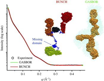
Fig. 9. Experimental SAXS curves (black circles) and scattering profiles computed from the models of a multidomain protein reconstructed by the rigid-body modeling using BUNCH (red line; Petoukhov & Svergun, Reference Petoukhov and Svergun2005) and ab-initio model using the program GASBOR (green line; Svergun et al. Reference Svergun, Petoukhov and Koch2001a). The secondary structural elements of the known atomic structures of the single modules are shown by a multicolor ball representation (yellow, gold, gray, red). Restored linker conformations between the modules are displayed by a blue beads representation and varied from run to run. Single best-fit models did not fit the smallest q region (q<0·03 Å−1) well, but fits involving multiple models did. The position of the unknown structure of the small domain has been modeled as the globular region at the position correlated with its position in the sequence (marked with the arrow). One GASBOR model is shown as gold beads superposed on the average shape shown as light blue spheres.
Table 3. Reconstruction of missing components

4.2.3 Computational docking combined with SAXS data
Atomic structures have long held the promise of allowing the structures of unknown complexes to be determined computationally. Substantial effort has been directed towards using only chemical and geometric parameters to determine docking sites (Mandell et al. Reference Mandell, Roberts, Pique, Kotlovyi, Mitchell, Nelson, Tsigelny and Ten Eyck2001; Bonvin, Reference Bonvin2006); however, this problem has not proven to be simple. Computational docking has two major challenges: (1) dealing with flexibility in macromolecules in a computationally practical manner and (2) determining an appropriate scoring function that successfully distinguishes correct solutions. A number of different strategies have been developed to introduce flexibility. Protocols allowing some degree of interpenetration of the molecules (‘soft docking’), side-chain flexibility, and truncating surface side-chains have been developed (Schnecke et al. Reference Schnecke, Swanson, Getzoff, Tainer and Kuhn1998; Palma et al. Reference Palma, Krippahl, Wampler and Moura2000; Chen et al. Reference Chen, Li and Weng2003; Heifetz & Eisenstein, Reference Heifetz and Eisenstein2003; Li et al. Reference Li, Chen and Weng2003). Additionally, docking has also employed ensembles of conformation (Smith et al. Reference Smith, Sternberg and Bates2005) from NMR structure determination (Dominguez et al. Reference Dominguez, Bonvin, Winkler, van Schaik, Timmers and Boelens2004), MD simulations (Rajamani et al. Reference Rajamani, Thiel, Vajda and Camacho2004), NMA (Mustard & Ritchie, Reference Mustard and Ritchie2005), or residual dipolar coupling (Tai, Reference Tai2004). A number of web servers generate conformational ensembles specifically for docking (Lei et al. Reference Lei, Zavodszky, Kuhn and Thorpe2004; Suhre & Sanejouand, Reference Suhre and Sanejouand2004; Barrett & Noble, Reference Barrett and Noble2005). Regardless of the protocol involved, an energy minimization is frequently run for top solutions to resolve steric clashes at the interface (Li et al. Reference Li, Chen and Weng2003).
SAXS can provide an experimental target function to score hits from the docking search and can substantially aid in the problem of development of scoring functions that successfully distinguish between good and bad solutions. For example, this combination has been used to show that the histone-like domain of the Ras activator son of sevenless folds onto a helical linker between two other son-of-sevenless domains (SOS; Sondermann et al. Reference Sondermann, Nagar, Bar-Sagi and Kuriyan2005). In this work, the docking of the SOSDH-PH-cat and SOSHistone crystal structures was performed separately from comparisons to SAXS results. Of the top 40 docking solutions, the top-scoring solution was also the best fit to the SAXS. Computation docking was also used to generate 100 dimeric structures of purine nucleoside phosphorylase and to verify that the crystallographic trimer was the assembly state in solution (Filgueira de Azevedo et al. Reference Filgueira de Azevedo, dos Santos, dos Santos, Olivieri, Canduri, Silva, Basso, Renard, da Fonseca, Mendes, Palma and Santos2003). We anticipate that computational docking of the supramolecular complexes and validation of models by SAXS will become a particularly powerful combination.
4.2.4 Differences in crystallographic and solution structures
The ability to directly compare atomic models to SAXS curves is a remarkably useful tool for deciphering the influences that the crystal lattice has on the observed structure. The crystal structure is likely the lowest energy state within the lattice and under crystallization conditions; however, it not necessarily the lowest energy state in solution. Many studies have suggested that the effects of the crystal lattice do not alter the folding of domains, but rather influence the conformations adopted by flexible termini or linkers between domains. Moreover, proteins that undergo allosteric rearrangements and have multiple stable conformations separated by small energy differences can be affected by lattice forces. The classic example for incompatibility between crystal lattices and conformational states is the cracking of reduced deoxyhemoglobin crystals upon the addition of oxygen (Perutz et al. Reference Perutz, Bolton, Diamond, Muirhead and Watson1964). By their very nature, crystal structures tend not to reveal the flexibility of the crystallized macromolecules. Crystal structures, such as for the c-Abl protein kinase (PDB id 1opl; Nagar et al. Reference Nagar, Hantschel, Young, Scheffzek, Veach, Bornmann, Clarkson, Superti-Furga and Kuriyan2003) that has two molecules in the asymmetric unit with substantially different domain arrangements tend to be the exceptions, so we favor continued research to optimize the combination of computational searches and SAXS data to characterize solution conformations.
A naive assumption is that crystallization will mostly force macromolecules to adopt a more compact structure. SAXS has revealed that crystallographically induced compaction is likely to be frequent, such as with the ligand-bound ‘relaxed’ state (but not the unliganded ‘tense’ state) of aspartate transcarbamoylase. These differences, however, could be modeled by small rigid-body subunit rotations on the order of 10 degrees (reviewed in Koch et al. Reference Koch, Vachette and Svergun2003). Despite these sorts of results, compaction by the lattice is not the only possible effect. For example, in a study of four thiamine diphosphate-dependent enzymes, one was found to be identical in the crystal and in solution, two appeared to be less compact in solution, and one complex with weaker subunit interactions was clearly more compact in solution (Svergun et al. Reference Svergun, Petoukhov, Koch and Koenig2000).
The differences between solution and crystal structures can be important for deciphering biological mechanisms. For example, the single conformation of the dimeric bacterial DNA mispair recognition protein MutS is likely constrained by lattice forces, despite the fact that multiple states are expected from biochemical results. MutS recognizes mispairs in DNA when in a nucleotide-free or ADP-bound state. Binding of ATP by bacterial or eukaryotic versions of the DNA–MutS complex induces a state in which the protein acts like a rigid ring that can freely diffuse along the length of the DNA and is no longer restricted to the mispair (Mendillo et al. Reference Mendillo, Mazur and Kolodner2005). Crystal structures of MutS–DNA complexes with ATP or ATP analogs have yet to reveal the conformational changes anticipated from biochemical studies (Lamers et al. Reference Lamers, Georgijevic, Lebbink, Winterwerp, Agianian, de Wind and Sixma2004). These predicted domain motions that would allow the two halves of the composite ATP-binding pockets to engage with their bound nucleotide have been anticipated by the effects of dominant mutations in the eukaryotic homologs (Hess et al. Reference Hess, Gupta and Kolodner2002) and studies in related systems for which both states are known (Hopfner et al. Reference Hopfner, Karcher, Shin, Craig, Arthur, Carney and Tainer2000). Regardless of whether or not these conformational changes are incompatible with the crystal lattice or due to the concentration effects of the trapped DNA, attempts to decipher these conformational changes have not yet been successful through crystallography alone. Properly assessing these conformational changes in the case of the efficient DNA repair machinery is important as toxins that interfere with the repair machinery are expected to be more dangerous to public health than toxins that directly damage DNA (McMurray & Tainer, Reference McMurray and Tainer2003).
4.2.5 Determining biological assemblies in crystal structures
Crystallization typically requires the formation of symmetric contacts that exist solely in the crystal and may not be important in biology. However biologically relevant multimers can also be symmetric, and biologically relevant symmetry operators can also be part of the underlying symmetry of the crystal structure so the contents of the asymmetric unit cannot be used as a guide for the biological assembly. Thus, crystallographers must decipher which macromolecular contacts mediate multimerization in solution and which are only crystal contacts.
In many cases identifying the biological multimer can be a difficult problem. Systematic investigation of atomic resolution structures has shown that authentic interfaces tend to be large and involve hydrophobic interactions on the surfaces of the protein (Jones & Thornton, Reference Jones and Thornton1996) and tend to be better packed than crystal contacts (Li et al. Reference Li, Keskin, Ma, Nussinov and Liang1985; Getzoff et al. Reference Getzoff, Tainer and Olson1986; Bahadur et al. Reference Bahadur, Chakrabarti, Rodier and Janin2004; Keskin et al. Reference Keskin, Ma and Nussinov2005). Additionally, these interfaces are less hydrated (Rodier et al. Reference Rodier, Bahadur, Chakrabarti and Janin2005) and tend to have greater sequence conservation (Valdar & Thornton, Reference Valdar and Thornton2001a, Reference Valdar and Thorntonb) with frequent tryptophans, phenylalanines, and methionines (Ma et al. Reference Ma, Elkayam, Wolfson and Nussinov2003). These analyses, although useful in the absence of other information, are theoretical in nature. SAXS data collected on the biologically relevant assemblies in solution has the potential to provide experimental information to help test and identify the biologically relevant interfaces in the crystal.
Identifying biological dimers is particularly difficult, as crystallographic symmetries tend to generate many dimeric interactions. For example, the bacterial mismatch repair protein MutL is known to form functional dimers. MutL is comprised of an N-terminal ATPase domain, a flexible internal linker, and a C-terminal domain that mediates constitutive dimerization (Drotschmann et al. Reference Drotschmann, Aronshtam, Fritz and Marinus1998). The dimeric C-terminal domain crystallized in the space group P4322 with four different dimer interfaces (PDB id 1x9z; Guarne et al. Reference Guarne, Ramon-Maiques, Wolff, Ghirlando, Hu, Miller and Yang2004). Two interfaces have remarkably small buried surface areas, but two others were more sizable. The dimer interface proposed by Guarne et al. later proved to be incorrect, whereas the other large dimer interface was consistent with crosslinking experiments and identifiable by computations analysis of packing (Kosinski et al. Reference Kosinski, Steindorf, Bujnicki, Giron-Monzon and Friedhoff2005). The biologically relevant dimer is more extended than the dimers generated by crystal contacts, and theoretical calculations suggest that SAXS could have easily distinguished it by size (R G=34·1 Å, D max=120 Å vs. R G=28·1 Å, D max=80 Å) as well as by the P(r) function that is characteristic of an elongated shape, having a peak at short distances and a long extended tail (R G=28·1 Å, D max=80 Å) (Fig. 10).

Fig. 10. SAXS could have readily distinguished between alternative dimer structures of the C-terminus of MutL observed in the crystal structure (PDB id 1x9z; Guarne et al. Reference Guarne, Ramon-Maiques, Wolff, Ghirlando, Hu, Miller and Yang2004). (a) Each of the four different dimers has remarkably different overall shapes, giving rise to measurable differences in SAXS and parameters such as R G and D max. Dimer 1, with a buried surface area of the monomer of 755 Å2, is the asymmetric unit of the crystal, whereas dimer 2, with a buried surface area of 923 Å2, is the solution dimer assembly (Kosinski et al. Reference Kosinski, Steindorf, Bujnicki, Giron-Monzon and Friedhoff2005). (b) Theoretical P(r) functions calculated for dimer 1 (black) and dimer 2 (red) are readily distinguished. Dimer 1 has a characteristic globular P(r) that is bell-shaped, whereas dimer 2 has a characteristic extended P(r) with an early peak and a long tail.
A more insidious challenge is when the authentic multimer does not exist in the crystal at all. Generating a solution assembly model given only the high resolution structure of a subunit is possible with SAXS data, and modeling assemblies with SAXS data will be discussed below. But before modeling can be performed, it is critical to identify that the biologically relevant assembly is not present in the crystal and to recognize that modeling must be done in the first place. In these cases, the lack of agreement between SAXS data collected on multimers in solution and theoretical scattering curves calculated from assembles observed in the crystals could be an important clue. For example, the hexameric assembly for the Holliday junction ATPase motor RuvB could be characterized by SAXS results in combination with the crystal structure of the subunit from a non-biologically relevant screw assembly (Putnam et al. Reference Putnam, Clancy, Tsuruta, Gonzalez, Wetmur and Tainer2001).
One particularly difficult problem was identifying the biological dimer of ATP-binding cassette (ABC) transporters (Fig. 11). ABC transporters couple ATP hydrolysis with the transport of ligands across membranes and include the cystic fibrosis transmembrane regulator. The nucleotide-binding domains of the ABC ATPase transporters were known to dimerize. The first of these structures, the Salmonella typhimurium histidine permease HisP was crystallized in the space group P43212 with two symmetry-related dimers in the crystal packing (PDB id 1b0u; Hung et al. Reference Hung, Wang, Nikaido, Liu, Ames and Kim1998); the largest dimer interface was proposed to be the biologically relevant one. Other transporter ABC ATPases were solved later, including the Thermococcus litoralis maltose transporter MalK (PDB id 1g29; Diederichs et al. Reference Diederichs, Diez, Greller, Mueller, Breed, Schnell, Vornrhein, Boos and Welte2000), and the Methanococcus jannaschii ABC ATPases MJ0796 (PDB id 1f3o; Yuan et al. Reference Yuan, Blecker, Martsinkevich, Millen, Thomas and Hunt2001) and MJ1267 (PDB id 1g6h and 1gaj, Karpowich et al. Reference Karpowich, Martsinkevich, Millen, Yuan, Dia, MacVey, Thomas and Hunt2001). Remarkably, each of these ABC ATPases had dimers generated by crystallographic symmetry, yet none shared common dimer interfaces. The biologically relevant dimer was first proposed using sequence analysis and the structure of the HisP monomer (Jones & George, Reference Jones and George1999). Dimerization generates an ‘ATP sandwich’ with the active site being made up of a Walker A ATP-binding and hydrolysis site on one molecule and an ABC ATPase ‘signature’ motif from the other subunit. These interfaces were first observed crystallographically in the ABC ATPase domains from the DNA repair proteins Rad50 (PDB id 1f2u; Hopfner et al. Reference Hopfner, Karcher, Shin, Craig, Arthur, Carney and Tainer2000) and MutS (PDB id 1e3m; Lamers et al. Reference Lamers, Perrakis, Enzlin, Winterwerp, de Wind and Sixma2000; PDB id 1ewq; Obmolova et al. Reference Obmolova, Ban, Hsieh and Yang2000), and the Rad50 structure in particular was subsequently used for modeling of the ABC transporters. The inference that the membrane transporters shared the Rad50/MutS dimer assembly was later established by the crystal structure of the E. coli BtuCD heterotetramer (PDB id 1l7v; Locher et al. Reference Locher, Lee and Rees2002).
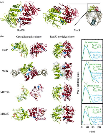
Fig. 11. SAXS has the potential to indicate mismatches between the dimers in the ABC ATPase assemblies observed in crystal and with their solution conformation, if dimeric states could have been stabilized for solution scattering. (a) The biological dimeric assemblies of the ABC ATPases were first observed with the DNA repair proteins Rad50 (PDB id 1f2u; Hopfner et al. Reference Hopfner, Karcher, Shin, Craig, Arthur, Carney and Tainer2000) and MutS (PDB id 1e3m, Lamers et al. Reference Lamers, Perrakis, Enzlin, Winterwerp, de Wind and Sixma2000; PDB id 1ewq, Obmolova et al. Reference Obmolova, Ban, Hsieh and Yang2000) that were normally stable as dimers in solution. Subunits are displayed as yellow and red ribbons; bound nucleotides are orange ball-and-stick models, and blue ribbons indicate the position of the signature motif that forms the second half of the ATP-binding surface. (b) Different crystallographic dimers were observed for HisP, MalK, MJ0796, and MJ1267 [PDB ids 1b0u, 1g29, 1f3o, 1g6h (Hung et al. Reference Hung, Wang, Nikaido, Liu, Ames and Kim1998; Diederichs et al. Reference Diederichs, Diez, Greller, Mueller, Breed, Schnell, Vornrhein, Boos and Welte2000; Karpowich et al. Reference Karpowich, Martsinkevich, Millen, Yuan, Dia, MacVey, Thomas and Hunt2001; Yuan et al. Reference Yuan, Blecker, Martsinkevich, Millen, Thomas and Hunt2001)] that lack special positioning of the signature motifs. Theoretical P(r) scattering curves clearly distinguish between the crystallographically observed dimers and those modeled using the Rad50 assembly.
SAXS can be used to distinguish between alternative assemblies in different crystal structures. The bacterial HslUV chaperone/protease complex had been observed in two distinct crystallographic assemblies (Fig. 12; Bochtler et al. Reference Bochtler, Hartmann, Song, Bourenkov, Bartunik and Huber2000; Sousa et al. Reference Sousa, Trame, Tsuruta, Wilbanks, Reddy and McKay2000). In the center of both assemblies was an HslV hexamer, but in the two different crystal forms the globular N- and C-terminal domains of HslU were either packed against HslV (PDB id 1g3i; Sousa et al. Reference Sousa, Trame, Tsuruta, Wilbanks, Reddy and McKay2000) or held away from HslV by an extended internal domain (PDB id 1doo; Bochtler et al. Reference Bochtler, Hartmann, Song, Bourenkov, Bartunik and Huber2000). The P(r) functions for these different assemblies and hence their X-ray scattering were easily distinguishable and SAXS revealed that in solution the globular N- and C-terminal domains of HslU pack against HslV and that the extended HslU domain extends into solvent (Sousa et al. Reference Sousa, Trame, Tsuruta, Wilbanks, Reddy and McKay2000).

Fig. 12. The two different HslUV protease/chaperone assemblies observed crystallographically have different orientations of the HslU hexamers (green) that interact on both sides of the double-ringed HslV dodecamer (gold). In the first, the globular domains of HslU are separated from HslV, giving a bimodal P(r) function with a R G of 90 Å and a D max of 265 Å (PDB id 1doo; Bochtler et al. Reference Bochtler, Hartmann, Song, Bourenkov, Bartunik and Huber2000). In the second, the globular domains of HslU pack against HslV, giving a monomodal P(r) function with a R G of 65 Å and a D max of 220 Å (PDB id 1g3i; Sousa et al. Reference Sousa, Trame, Tsuruta, Wilbanks, Reddy and McKay2000). The experimental P(r) function (not shown; Sousa et al. Reference Sousa, Trame, Tsuruta, Wilbanks, Reddy and McKay2000) strongly argues for a monomodal distribution and the more compact 1g3i-like assembly (after Sousa et al. Reference Sousa, Trame, Tsuruta, Wilbanks, Reddy and McKay2000).
Finally, SAXS can establish the validity of weak assemblies observed in crystal packing that might be ignored as artifacts of the crystallization process. The E. coli mismatch repair protein MutS forms a dimer that recognizes mispairs in DNA. At high protein concentrations, MutS forms tetramers that depend upon the presence of the C-terminal 53 amino acids (Bjornson et al. Reference Bjornson, Blackwell, Sage, Baitinger, Allen and Modrich2003). Fusions of this C-terminal domain onto maltose binding protein (MBP) mediated its tetramerization, and the crystal structure revealed a helix–loop–helix domain that made a symmetric interaction to form a tight dimer (PDB id 2ok2; Mendillo et al. Reference Mendillo, Putnam and Kolodner2007). A potential tetramer contact was observed in the crystal form; however, the interface was small and weakly packed. Despite this, SAXS data collected on the MBP fusion protein and subsequent mutagenesis of salt bridges that stabilized it revealed that the tetramer in solution closely resembled the assembly observed crystallographically. Similarly, a combination of SAXS, ultracentrifugation, and EM was used to validate the biologically relevant Mre112/Rad502 heterotetrameric DNA processing head used in double-strand break repair, whose structure was inferred from the atomic resolution structures of Mre11, Rad50, and biochemical results (Hopfner et al. Reference Hopfner, Karcher, Craig, Woo, Carney and Tainer2001).
4.3 Modeling atomic assemblies using ab-initio SAXS structures
Substantial theoretical and practical work has gone into establishing that three-dimensional reconstructions can be derived from the one-dimensional SAXS curve (Section 4.3.1). Successful reconstructions generate low-resolution envelopes that are analogous to averaged reconstructions generated by EM. Similarly, many of the tools used in EM for fitting known atomic assemblies into these envelopes can also be used for docking atomic structures in a rigid-body fashion (Section 4.3.2) or using methods that allow flexibility to be introduced into the atomic models (Section 4.3.3). Introducing flexibility in the atomic model is valuable in situations where the three-dimensional reconstruction involves a state of the macromolecule that is different from the state that was used for determining the atomic resolution structure. The ab-initio envelope reconstruction protocols substantially differ from those using atomic models described above (Section 4.2). In these protocols, all of the independent experimental values extracted from the SAXS curves are used for generating an overall envelope, which frequently has a uniqueness problem. Depending on the system, we suggest that rigid-body modeling of a small number of subunits is a more powerful use of the information content in SAXS curves than ab-initio envelope reconstruction; however, these modeling methods are independent and can be performed in parallel. Similar answers deduced by each technique can help give confidence in the solutions; although we believe that ab-initio models are best treated as hypotheses to be tested by additional experimentation (Fig. 13).

Fig. 13. SAXS models of the complexed cellulase can be reconstructed using different methods. (a) Ab-initio model reconstructed by spherical harmonics using SASHA (Svergun et al. Reference Svergun, Volkov, Kozin and Stuhrmann1996). (b) Densely packed beads model using DAMMIN (Svergun, Reference Svergun1999). (c) Model calculated with GASBOR (Petoukhov et al. Reference Petoukhov, Eady, Brown and Svergun2002) (d) Reconstruction of one missing module using dummy residues with CREDO (green) (Petoukhov et al. Reference Petoukhov, Eady, Brown and Svergun2002). The secondary structural elements of fixed known atomic structure are in gray. (e) Rigid-body modeling applied on the knowing atomic structures (gray) in the combination with ab-initio modeling of the linkers region (cyan) using BUNCH (Petoukhov & Svergun, Reference Petoukhov and Svergun2005). (f) Rigid-body modeling using conformational sampling. Thousands of possible atomic models, by applying molecular dynamics on the linker region (blue) have been used in an exhaustive search of the best-fit conformation. One hundred conformations (yellow) are shown superimposed on the catalytic module (gray) (Hammel et al. Reference Hammel, Fierobe, Czjzek, Finet and Receveur-Brechot2004a).
4.3.1 Calculation of ab-initio SAXS envelopes
Several programs have been created for the purpose of calculating so called ab-initio shapes from scattering profiles (Table 4). In practice many of these programs use information external to the scattering profiles and the term ab initio solely refers to lack of a pre-defined input structure. These programs implicitly or explicitly assume the shape is a continuous object, which substantially reduces the search space. We do not attempt to provide detailed descriptions of these programs here and the citations listed in Table 4 should be referenced. The general approach taken by these programs is to propose shapes, calculate scattering curves or P(r) functions and optimize the agreement to the experimental data (Fig. 13).
Table 4. Ab-initio SAXS envelope reconstruction programs

Many of the early programs restricted searches to shapes defined by a small number of parameters. For example, R G can be thought of as describing an ab-initio model with a single parameter: a spherical envelope of radius r=(5/3)½R G. Whole-body methods approach the problem by attempting to fit X-ray scattering using spheres, oblate, prolate, and triaxial ellipsoids and are also used for modeling hydrodynamic properties (Rallison & Harding, Reference Rallison and Harding1985). A modern version of this algorithm that can also combine several simple shapes is available with the program ELLSTAT (Heller, Reference Heller2006). Spherical harmonics also have been used (Svergun & Stuhrmann, Reference Svergun and Stuhrmann1991) as implemented in SASHA (Fig. 13a; Svergun et al. Reference Svergun, Volkov, Kozin and Stuhrmann1996). However, spherical harmonics descriptions cannot properly represent all shapes, such as structures with cavities or holes. In the specialized case of icosohedrally symmetric virus particles, icosohedral harmonics have also been employed to describe low-resolution structures (Zheng et al. Reference Zheng, Doerschuk and Johnson1995).
Recently, a number of over-parameterized methods have been used for ab-initio shape determination (Volkov & Svergun, Reference Volkov and Svergun2003). These methods attempt to generate a bead model (or dummy atom model) to fill a volume consistent with the experimental scattering. External constraints, such as smoothness, connectivity, and particle symmetry have been used to reduce the search space (Koch et al. Reference Koch, Vachette and Svergun2003). The number of possible arrangements increases combinatorially, so all programs use computational tricks to search through the solution space including Monte Carlo approaches, genetic algorithms, and simulated annealing (Table 4). Several programs fit directly to the scattering data involving a Fourier transform for each shape proposed. This becomes computationally intensive and cheap methods of calculating scattering curves from proposed shapes have been developed (Section 4.1).
Shape-restoration programs using bead models do not uniquely define the position of each bead within a volume, nor do the beads represent positions of specific residues. Rather, the bead positions are non-unique and define a volume for the scattering particle, as illustrated by six independent GASBOR reconstructions of the human OGG1 DNA glycosylase/lyase (Fig. 14). Each of the reconstructions fits the experimental scattering equally well and describes similar shapes. GASBOR is designed specifically for proteins (though modeling of other macromolecules is possible); dummy atoms have radii approximating amino acids with penalties imposing chain connectivity. In the case of OGG1, the envelope generated by averaging the different GASBOR runs fits the volume and shapes the truncated crystal structure (Fig. 14).
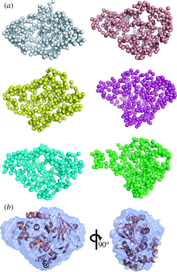
Fig. 14. GASBOR reconstructions of OGG1, a 39 kDa protein critical to the recognition and repair of oxidized guanine in double-stranded DNA by the DNA base-excision repair pathway. (Protein courtesy of Tapas Hazra and Sankar Mitra University of Texas, Galveston, reconstructions for functional analyses in collaboration with Cynthia McMurray.) (a) Six independent runs of GASBOR showing the variation among models all of which produce scattering curves in agreement with the experimental data. Each model is composed of dummy atoms whose radii approximate those of amino acids. Data were collected at a concentration of 5 mg/ml with a 30-s exposure. (b) The crystal structure of a truncated version of OGG1 fits well within the ab-initio SAXS envelope defined by the average of the six GASBOR runs. Each run takes around two hours on computers typically found in most laboratories.
The final resolution attainable from ab-initio envelopes varies with data quality, the program used, particle size, shape and flexibility (Section 5.6). Several studies have compared available programs (Takahashi et al. Reference Takahashi, Nishikawa and Fujisawa2003; Zipper & Durschschlag, Reference Zipper and Durschschlag2003); however, a systematic study on the accuracy of ab-initio envelopes has not been conducted. Figure 6 shows 10 ab-initio reconstructions and the average shape from the highly flexible detergent solubilized apoB-100 generated by DAMMIN. A larger variation exists between the models in comparison to OGG1 (Fig. 14); although, the overall dimensions are in agreement and suggest relative domain motions. Very flexible structures typically have fewer features in their scattering profiles, which can be fit by a greater variety of shapes. A comparison of the output of multiple independent modeling runs (at least 6–10) provides some measure of the uniqueness of the models.
One parameter used to characterize the agreement among models is the normalized spatial discrepancy (NSD) (Kozin & Svergun, Reference Kozin and Svergun2001). Briefly, if models 1 and 2 are expressed in two sets of points P 1={p 1i, i=1, …, N 1} and P 2={p 2i, i=1, …, N 2}, then, NSD between P 1 and P 2 is defined as
![\rho \lpar P_{\setnum{1}} \comma P_{\setnum{2}} \rpar \equals \left\{ {{1 \over 2}\left[ {{1 \over {N_{\setnum{1}} d_{\setnum{2}} ^{\setnum{2}} }}\sum\limits_{i \equals \setnum{1}}^{N_{\setnum{1}} } {\rho ^{\setnum{2}} \lpar\hskip2 p_{\setnum{1}i} \comma P_{\setnum{2}} \rpar \plus {1 \over {N_{\setnum{2}} d_{\setnum{1}}^{\setnum{2}} }}\sum\limits_{i \equals \setnum{1}}^{N_{\setnum{2}} } {\rho ^{\setnum{2}} \lpar\hskip2 p_{\setnum{2}i} \comma P_{\setnum{1}} } } \rpar } \right]} \right\}^{\textstyle\frac{1}{2}}\comma](https://static.cambridge.org/binary/version/id/urn:cambridge.org:id:binary:20151023075232796-0121:S0033583507004635_eqnU39.gif?pub-status=live)
where N i is the nuber of points in P i, d is the average distance between neighboring points in P i, and ρ(p 1i, P 2) is the distance from arbitrary points, p 1i, in P 1 to the nearest point in P 2. NSD is 0 for identical models. NSD enables quantitative comparison of similarities of models if the modes have the same resolutions, but it is not straightforward to compare similarities of models with different resolutions because N i and d are very different. In these cases, using the program SITUS, which was originally developed for EM, is more appropriate (Wriggers et al. Reference Wriggers, Milligan and McCammon1999; Wriggers & Chacon, Reference Wriggers and Chacon2001).
The combination of multiple runs and external constraints has been remarkably successful for the low-resolution envelope reconstruction of many systems (Fig. 15). Imposing correct symmetry greatly enhances the resolution of final results. In general, symmetry information will need to be introduced from external information. However, in the case of the cytosolic portion of a voltage-gated potassium channel (Pioletti et al. Reference Pioletti, Findeisen, Hura and Minor2006), the fourfold symmetry could be derived from the scattering using GASBOR, as shown by the result of imposing various symmetries (Fig. 16). Each of the five symmetries shown was run eight times resulting in a total of 40 GASBOR runs. Each run required 12 h of computer time for the 1288 amino-acid complex. In this case, the overall shape could be reconstructed even when fourfold symmetry was not explicitly enforced. Imposed symmetries below and including fourfold-derived shapes with similar χ2 agreement to the experimental data. Imposing higher symmetries resulted in noticeably higher χ2 values and marginally poorer fits to the data. On the other hand symmetries of fourfold and higher had low NSD values, implying a much smaller variation in shapes. An imposed fourfold symmetry optimized both the χ2 agreement and NSD values (Fig. 16f). We note that the mass was a critical parameter required as input for this study, and the ability to determine overall symmetry by SAXS will likely depend greatly on the overall shape of the target. In this case, the dramatic X-shape of the potassium channel, which is apparent even at extremely low resolutions, was likely critical for determining the proper symmetry.

Fig. 15. Crystallographic and SAXS based models of DNA ligase-PCNA complex. (a) A model of human DNA-ligase-PCNA postulated from two independent crystal structures: human PCNA (purple surface PDB id 1w69; Kontopidis et al. Reference Kontopidis, Wu, Zheleva, Taylor, McInnes, Lane, Fischer and Walkinshaw2005) and human ligase I (green) complexed with nicked DNA (orange, PDB id 1x9n; Pascal et al. Reference Pascal, O’Brien, Tomkinson and Ellenberger2004). The model assumes the two ring-like structures are co-axial around DNA. B. The averaged ab-initio SAXS model derived from experimental SAXS data of the Sulfolobus solfataricus ligase-PCNA complex without DNA (purple transparent surface) superposed on the complex reconstructed from the ligase (PDB id 2hiv) and PCNA (PDB id 2hii) models using SASREF (Petoukhov & Svergun, Reference Petoukhov and Svergun2005). Ab-initio shapes were calculated by GASBOR (Svergun et al. Reference Svergun, Petoukhov and Koch2001a) and average using DAMAVER (Volkov & Svergun, Reference Volkov and Svergun2003) (after Pascal et al. Reference Pascal, Tsodikov, Hura, Song, Cotner, Classen, Tomkinson, Tainer and Ellenberger2006).
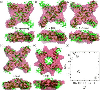
Fig. 16. SAXS envelopes calculated with different point-group symmetries determined from experimental data from the cytosolic portion of a voltage-gated potassium channel (a tetramer generated from two heterodimers) and overlaid on the crystal structure (Pioletti et al. Reference Pioletti, Findeisen, Hura and Minor2006). Each of the envelopes is the result of averaging eight GASBOR (Svergun et al. Reference Svergun, Petoukhov and Koch2001a) runs and is shown in two orientations, 90° apart. Models were calculated with the point group symmetries of (a) p1 (no symmetry), (b) p2 (one twofold), (c) p222 (three perpendicular twofolds), (d) p4 (one fourfold), and (e) p8 (one eightfold). For each applied symmetry indicated by the value in the circle, the discrepancy between the individual models (NSD; Section 4.3.1) is plotted against the average agreement with the experimental scattering (χ2; Section 4.1). The model generated with fourfold symmetry has nearly equivalent χ2 with lower symmetry models but also has low NSD values. All models suggest a fourfold symmetric structure, excepting the model forced to have p8 point-group symmetry.
One of the temptations of ab-initio programs is that they require much less information and are easier to run. However, atomic resolution information provides substantially more restraints on possible solutions and is in our opinion the future of SAXS computational development. Ab-initio derived models can support models built with or proposed by other methods. Moreover, ab-initio structures can be used directly to build atomic models through rigid-body (Section 4.3.2) or flexible (Section 4.3.3) docking into the envelopes.
4.3.2 Rigid-body docking into low-resolution envelopes
A candidate ab-initio SAXS structure is essentially a low-resolution envelope to which an atomic structure may be docked. Finding a manual best fit using specifically developed SAXS software (Kozin et al. Reference Kozin, Volkov and Svergun1997; Konarev et al. Reference Konarev, Petoukhov and Svergun2001) or with standard molecular graphics programs using envelopes expressed as atomic positions can be a surprisingly challenging process. The program SUPCOMB (Kozin & Svergun, Reference Kozin and Svergun2001) automatically superimposes atomic structures with dummy atom models; however, this problem is essentially the same as that faced when fitting high-resolution structures into EM maps. Substantial progress has been made in the EM community in this area (Volkmann & Hanein, Reference Volkmann and Hanein1999; Roseman, Reference Roseman2000; Rossmann, Reference Rossmann2000; Wriggers & Chacon, Reference Wriggers and Chacon2001; Chacon & Wriggers, Reference Chacon and Wriggers2002; Navaza et al. Reference Navaza, Lepault, Rey, Alvarez-Rua and Borge2002; Craig et al. Reference Craig, Volkmann, Arvai, Pique, Yeager, Egelman and Tainer2006), and the EM program SITUS (Wriggers et al. Reference Wriggers, Milligan and McCammon1999) has also been used for SAXS (Rosenberg et al. Reference Rosenberg, Deindl, Sung, Nairn and Kuriyan2005). In SITUS the distribution of atoms within the high-resolution structure as well as the low-resolution reconstructions are approximated by a small number of vectors that are calculated by vector quantization. Vector quantization-based fitting is limited to cases in which all density in the SAXS envelope is accounted for by the atomic model. In practice missing or disordered regions of the atomic model need to be modeled before vector quantization-based fitting can be applied (Volkmann & Hanein, Reference Volkmann and Hanein2003). Additionally, more accurate correlation-based approaches have been proposed. In these methods the solution sets lead to the possibility of defining confidence intervals and error margins for the fitting parameters, which is particularly important in the context of docking atomic structures into low-resolution density maps as no independent information is available on how a correct fit should look (Volkmann & Hanein, Reference Volkmann and Hanein2003).
The ability to align crystal structures into SAXS envelopes is particularly informative when there are functionally related conformational changes. For example, both symmetry and the existence of atomic resolution structures combined with SAXS analysis have provided substantial information regarding the mechanism by which the AAA+-ATPase p97 undergoes ATP-coupled conformational changes. Ab-initio reconstruction of SAXS envelopes for this hexameric ATPase with p3 or p6 point-group symmetry provided substantial information on conformational changes induced upon nucleotide binding (Davies et al. Reference Davies, Tsuruta, May and Weis2005). States induced by the non-hydrolysable analog AMP-PNP, the transition-state like mimic ADP-AlFx, ADP, and no nucleotide were readily distinguishable in GASBOR-generated envelopes and consistent with previous EM studies (Zhang et al. Reference Zhang, Shaw, Bates, Newman, Bowen, Orlova, Gorman, Kondo, Dokurno and Lally2000b; Rouiller et al. Reference Rouiller, DeLaBarre, May, Weis, Brunger, Milligan and Wilson-Kubalek2002; Beuron et al. Reference Beuron, Flynn, Ma, Kondo, Zhang and Freemont2003). Using the crystal structure of the ADP-AlFx bound state, different conformations were proposed, revealing a coordinated mechanism for transferring the energy of nucleotide hydrolysis through two parallel rings of domains.
Modeling atomic resolution structures into SAXS envelopes has been used to study the conformational states of the ATPase domain of the Aquifex aeolicus enhancer-binding protein NtrC1 in various nucleotide-bound states. NtrC1, which is also an AAA+-ATPase, acts upon a quiescent σ54–RNA polymerase complex to activate transcription initiation. Superposition of the ADP-bound crystal structure of the heptameric ATPase domain with low-resolution envelopes derived from SAXS with enforced sevenfold symmetry could be used to model the nucleotide control of different conformational states. In conjunction with EM, the authors demonstrated an ATP-bound state that stabilized the EBP–54–RNA polymerase complex, while subsequent hydrolysis and phosphate release drove the conformational changes necessary to generate an open polymerase/promoter complex (Chen et al. Reference Chen, Doucleff, Wemmer, De Carlo, Huang, Nogales, Hoover, Kondrashkina, Guo and Nixon2007).
4.3.3 Flexible docking into low-resolution envelopes
In addition to rigid-body fitting of domains into low-resolution envelopes, ab-initio SAXS envelopes, like experimental EM maps, may correspond to states that are different from the crystallized form of the macromolecule. Hence, computational techniques that can take single conformational states and account for potential flexibility during the docking protocols become quite useful. This problem has been faced frequently in EM studies and a variety of computational methods are currently being applied (Suhre et al. Reference Suhre, Navaza and Sanejouand2006). Large conformational changes have been shown to frequently correspond to highly collective movements that can be described by a small number of low-frequency normal modes of protein (Section 3.3; Tama & Sanejouand, Reference Tama and Sanejouand2001), and structures modified by NMA (Section 3.3) have been used for fitting EM density maps (Tama et al. Reference Tama, Miyashita and Brooks2004; Hinsen et al. Reference Hinsen, Reuter, Navaza, Stokes and Lacapere2005; Mitra et al. Reference Mitra, Schaffitzel, Shaikh, Tama, Jenni, Brooks, Ban and Frank2005). For example, the NORMA software package (Suhre et al. Reference Suhre, Navaza and Sanejouand2006) allows flexible fitting to EM maps and is well suited for SAXS envelopes; however, the SAXS envelopes generally need to be converted into synthetic EM envelopes with SITUS first (Wriggers et al. Reference Wriggers, Milligan and McCammon1999).
The elastic normal modes computed based on the low-resolution envelopes compare well with the normal modes obtained at atomic resolution (Tama et al. Reference Tama, Wriggers and Brooks2002; Chacon et al. Reference Chacon, Tama and Wriggers2003). Thus the motions of large macromolecular assemblies can be directly extracted from low-resolution envelopes derived from SAXS or EM, as has been shown for the DNA-dependent protein kinase and pyruvate dehydrogenase (Boskovic et al. Reference Boskovic, Rivera-Calzada, Maman, Chacon, Willison, Pearl and Llorca2003; Kong et al. Reference Kong, Ming, Wu, Stoops, Zhou and Ma2003). NMA has also been used to study the motion in free and complexed cellulase built from SAXS models (Hammel et al. Reference Hammel, Fierobe, Czjzek, Finet and Receveur-Brechot2004a) when submitted to the ElNémo server (Suhre & Sanejouand, Reference Suhre and Sanejouand2004). Computational methods other than NMA could be used to deform molecules to fit into these low-resolution envelopes; however, NMA has proven to be quite useful due to the efficiency for which altered conformations can be calculated.
4.4 Flexibility and conformational disorder measured by SAXS
Several forms of flexibility are crucial for the function of many macromolecular complexes and enzymes (Boehr et al. Reference Boehr, McElheny, Dyson and Wright2006). A common example are flexible linkers, such as those controlling the overall domain conformations and activation of protein kinases (Nagar et al. Reference Nagar, Hantschel, Seeliger, Davies, Weis, Superti-Furga and Kuriyan2006). In another example, analysis of the P(r) function demonstrated that the flexibly linked primase subunits dissociated when ionic strength was increased. This response to changes in ionic strength was linked to primase function (Corn et al. Reference Corn, Pease, Hura and Berger2005). A more dramatic form of flexibility is exemplified by a new class of important regulatory proteins, which do not have a single three-dimensional conformation and are either intrinsically unstructured or natively unfolded (Dyson & Wright, Reference Dyson and Wright2005). It has been estimated that over 50% of eukaryotic proteins contain unstructured regions that are over 40 amino acids in length (Vucetic et al. Reference Vucetic, Brown, Dunker and Obradovic2003), and growing evidence suggests that macromolecular flexibility will be an important part of the regulatory mechanism in many different biological systems.
While samples containing multiple conformations can be challenging to crystallize and tend to reach a single low-energy conformation when they do, they present no difficulties for data collection by SAXS. In combination with domain structures from X-ray crystallography and NMR and recent advances in computational approaches, SAXS has the potential to provide realistic information regarding large-scale structural rearrangements. The techniques described in Sections 4.2 and 4.3 focus on determining a single ‘best’ conformation. For particularly flexible samples, this conformation is unlikely to exist, and any single conformation of the macromolecule would be predicted to fit the scattering poorly. The real challenges for modeling this flexibility are the dramatic increase in the number of fittable parameters and the difficulties in incorporating multiple models during model refinement. The simplest case of conformational heterogeneity in SAXS is the presence of multiple well-defined conformations (Section 4.4.1), such as are observed during allosteric rearrangements. In contrast, assemblies containing linkers that allow for free, continuous motions of individual domains are more challenging to model (Section 4.4.2) and must be distinguished in SAXS from samples suffering from aggregation (Section 4.4.3).
4.4.1 Multiple well-defined conformations
Assuming that different conformational states do not interact, the resulting scattering from a mixed sample is a population-weighted average of scattering from individual states. This scattering poses a significant challenge for all shape reconstruction techniques. Nevertheless, data determined from the consensus population in solution, under a variety of conditions can be advantageous. A concern with cryo-EM is that an observed minor population overly biases the determined shape. This was dramatically demonstrated by cryo-EM and SAXS DNA bound and free structures of the important DNA damage response protein p53, which is mutated in 50% of all human cancer (Tidow et al. Reference Tidow, Melero, Mylonas, Freund, Grossmann, Carazo, Svergun, Valle and Fersht2007).
In general, the characterization of these mixed states by SAXS is most straightforward if the different states can be isolated independently and treated as homogeneous samples. Driving the population to a single conformation might be induced by buffer conditions or through binding specific ligands or substrates. For example, the dodecameric Ca2+/calmodulin-dependent protein kinase II (CaMKII) converts from a compact autoinhibited state to a loosely tethered state with independent kinase domains upon Ca2+ binding (Rosenberg et al. Reference Rosenberg, Deindl, Sung, Nairn and Kuriyan2005).
Alternatively, direct comparisons of different conformational states with theoretical scattering calculated from atomic-resolution structures has been quite successful in identifying and deconvoluting the relative fractions in the sample, such as with the archaeal secretion ATPase GspE (Fig. 17). The structure was solved as a mixed hexamer of open and closed conformational states of the component monomers (Yamagata & Tainer, Reference Yamagata and Tainer2007). Fitting of the solution X-ray scattering curves of the Mg2+ and AMP-PNP bound enzyme fit the experimental crystal structure less well than a computational hexamer generated from the closed state of the monomers alone. Moreover, the scattering of the ADP-bound state was well fit by a mixture of scattering from the crystal structure, the all-open model, and the all-closed model, demonstrating considerable flexibility in the system only using experimentally determined states of the monomer for modeling.
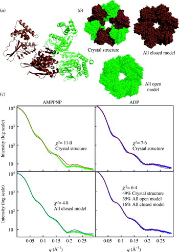
Fig. 17. Determination of the solution conformation of the hexameric archaeal secretion ATPase GspE from a combination of SAXS and crystallography. (a) Side view of the 2 alternating configurations of the ATPase GspE monomer bound to AMPPNP found in the hexameric structure determined via crystallography. (b) Top views of the crystal structure and two models proposed by modifying subunits to adopt either all open (brown) or all closed (green) conformations. (c) In solution the ATPase in excess AMPPNP adopts a conformation most similar to the all closed model while a solution with excess ADP is best described as a mixture of all the models (after Yamagata & Tainer, Reference Yamagata and Tainer2007).
Identifying that a solution contains a mixed population of macromolecules can be challenging and often requires additional information from other techniques such as native gel electrophoresis. Since R G2 corresponds to the average square distance of each scatterer from the center of the particle contributing to the scattering, mixed samples containing components with different R G values will yield observed R G's that are the square root of the weighted sum of the R G2 values of the different components. Thus, mixed populations continue to have linear Guinier regions (Heller, Reference Heller2005). Moreover, the signal indicating heterogeneity is highly dependent upon how much the conformational changes alter SAXS (Heller, Reference Heller2005). In the calculation of the collapse of calmodulin, for example, the 2·6 Å difference in R G and 20 Å differences in D max were readily apparent, even when simulated noise was added to the scattering curves. Ab-initio reconstructions of mixed populations show substantial conformational components of both extended and collapsed states. In contrast, the conformational changes involving protein kinase A, with a change in R G of 0·13 Å, were lost when noise was added to the theoretical scattering (Heller, Reference Heller2005). Therefore, SAXS studies of mixed populations that give rise to large changes in SAXS will be the most straightforward. For example, scattering power in the small-angle region goes by the square of the mass; hence, mixed populations of different multimeric states will be more readily identified. Similarly, unfolding of macromolecules involves large-scale changes in the overall structure and will dramatically change the observed scattering; thus, SAXS has been a method of choice for studying protein folding (Provencher & Glockner, Reference Provencher and Glockner1983; Doniach, Reference Doniach2001; Perez et al. Reference Perez, Vachette, Russo, Desmadril and Durand2001).
The best way to identify heterogeneity is by following it through titration of the states from one form to another or through situations in which atomic models are available so that they can be directly compared to the observed scattering. For example, SAXS has been used to follow large-scale changes due the pH-induced maturation of viral capsids of the HK97 bacteriophage and Nudaurelia capensis ω virus, which give rise to substantial changes in the SAXS curve (Canady et al. Reference Canady, Tsuruta and Johnson2001; Lee et al. Reference Lee, Gan, Tsuruta, Hendrix, Duda and Johnson2004). Moreover, several schemes have been used to prove the existence of transient, substrate-induced conformational changes and characterize them (Akiyama et al. Reference Akiyama, Fujisawa, Ishimori, Morishima and Aono2004; Goettig et al. Reference Goettig, Brandstetter, Groll, Gohring, Konarev, Svergun, Huber and Kim2005; Graille et al. Reference Graille, Zhou, Receveur-Brechot, Collinet, Declerck and van Tileurgh2005; Vestergaard et al. Reference Vestergaard, Sanyal, Roessle, Mora, Buckingham, Kastrup, Gajhede, Svergun and Ehrenberg2005; Nowak et al. Reference Nowak, Panjikar, Konarev, Svergun and Tucker2006a, Reference Nowak, Panjikar, Morth, Jordanova, Svergun and Tuckerb).
Using experimentally determined SAXS and theoretical scattering from individual components (form factors), volume fractions in each conformation can be determined by solving a systems of linear equations with the program OLIGOMER (Konarev et al. Reference Konarev, Volkov, Sokolova, Koch and Svergun2003). The bacterial class I release factors, for example, adopt a compact structure in the crystal, but unlike the crystal, the solution scattering is consistent with a population containing 92·5% in an open conformation and only 7·5% in the compact form (Vestergaard et al. Reference Vestergaard, Sanyal, Roessle, Mora, Buckingham, Kastrup, Gajhede, Svergun and Ehrenberg2005). Similarly, the transcriptional antiterminator LicT exhibits a heterogeneous population in solution with 61% being open and 39% being compact and active (Graille et al. Reference Graille, Zhou, Receveur-Brechot, Collinet, Declerck and van Tileurgh2005).
In addition to systems of linear equations, single-value decomposition (SVD; Press et al. Reference Press, Teukolsky, Vetterling and Flannery1992) can deconvolute SAXS data from mixtures. SVD was introduced into SAXS in the early 1980s (Fowler et al. Reference Fowler, Foote, Moody, Vachette, Provencher, Gabriel, Bordas and Koch1983) and has been applied to the problem of protein folding (Chen et al. Reference Chen, Hodgson and Doniach1996; Perez et al. Reference Perez, Vachette, Russo, Desmadril and Durand2001) as well as deconvoluting mixtures of protein–RNA complexes (Bilgin et al. Reference Bilgin, Ehrenberg, Ebel, Zaccai, Sayers, Koch, Svergun, Barberato, Volkov, Nissen and Nyborg1998) and transient protein conformations (Fetler et al. Reference Fetler, Tauc, Herve, Moody and Vachette1995). SVD requires multiple scattering curves collected from samples containing different populations of states. Unlike solving systems of linear equations, SVD does not require scattering curves from individual components, but in order to extract real scattering curves external information may be required, such as thermodynamic models for transitions.
In SVD, all the collected scattering profiles I n(q) are reduced to a common minimal basis set as described in the following equation:
where w jb jn is the weighting contribution of uj basis vector to I n(q), the nth experimentally determined scattering profile. Determining the values of basis vectors and the relative weights is accomplished through creating an M×N matrix A(M×N) where the N columns are the intensity values of the scattering profiles determined at M values of q. Such a matrix may be represented as A(M×N)=U(M×N) W(N×N) B(N×N) where U is also an M×N matrix containing the uj basis vectors, W is a diagonal N×N matrix composed of the so-called singular values w j and B is an N×N matrix containing b jn. Although U contains N vectors, only important basis vectors will have associated significant w j values. Many vectors in U will fit noise in the data rather than the significant parts of scattering profiles. Several commercially available mathematical packages have built-in SVD routines.
SVD will identify the minimum number of curves required to describe all the scattering profiles and can readily distinguish a system with a single transition from one with multiple transitions. Only two basis vectors were necessary to describe the scattering datasets collected from the allosteric enzyme aspartate transcarbamoylase measured in the presence of various substrate analogs, activators, and inhibitors (Fetler et al. Reference Fetler, Tauc, Herve, Moody and Vachette1995).
In an illustrative use of SVD, the temperature denaturation of neocarzinostatin was characterized by SAXS (Perez et al. Reference Perez, Vachette, Russo, Desmadril and Durand2001). At least three SVD basis vectors were required for a complete description of the unfolding, suggesting the presence of at least one intermediate state. With the scattering from the starting protein and the final unfolded state, they attempted to derive the scattering from the intermediate state by reprojecting the basis set. However, the derived scattering curve was degenerate, and the authors concluded that the folding pathway of neocarzinostatin involves an ensemble of related flexible intermediate states.
Another promising application of SVD is toward characterizing detergent solubilized membrane proteins (Lipfert & Doniach, Reference Lipfert and Doniach2007). The experimental matrix for SVD used SAXS data collected from different concentration ratios of membrane protein to detergent. All concentrations of detergents were above the critical micelle concentration. They reprojected the SVD vectors as scattering due to membrane protein–detergent complex, micelles, a micelle–micelle interaction component and a membrane protein–detergent to micelle interaction component. Of course the component of interest is the membrane protein–detergent complex. Although their experimental application using membrane protein TM0026 did not provide details on structural parameters other than R G, the potential to isolate the scattering profile of a membrane protein–detergent complex is very exciting and well worth further research effort.
SVD is potentially very powerful; however, some care must be taken in employing the technique. Robust analysis requires many scattering curves and relatively error-free data. Systematic errors from background subtraction among the data sets may cause particularly insidious problems for SVD, as some of the basis sets may be required to fit error rather than be truly representative of solutions. If background-subtracted data is used in the SVD analysis, great care must be taken in titration experiments to guarantee the buffer is properly matched to the solution for background subtraction. SVD is also particularly powerful for time-resolved experiments of induced conformational changes. Unfortunately, time-resolved experiments with short exposures also suffer from weaker signals. Finally, SVD identifies the minimum number of scattering curves and not necessarily all states that may exist (Koch et al. Reference Koch, Vachette and Svergun2003), which might be particularly problematic when a continuum of states exist, such as with partially unfolded peptides.
4.4.2 Conformational disorder explored by SAXS
In contrast to samples that can be described as containing multiple well-defined conformations, many multidomain proteins and protein complexes contain flexible linkers that allow them to adopt large numbers of conformations. This situation is substantially more complex to model; however, it is likely to be quite common for large numbers of eukaryotic proteins. For these types of samples, attempting shape reconstructions to derive a single model with a ‘best-fit’ conformation can be misleading and at best provides a model representing an average of the conformations. At times an averaged model can be informative. For example, SAXS studies of the c-Abl tyrosine kinase that is dysregulated by gene fusions in chronic myelogenous leukemia (Nagar et al. Reference Nagar, Hantschel, Seeliger, Davies, Weis, Superti-Furga and Kuriyan2006) have provided additional insight into the autoinhibition of the kinase. The N-terminal half of Abl is comprised of three domains connected by flexible linkers. Binding of the myristoylated N-terminus within a binding pocket on the protein generates a compact autoinhibitated state. SAXS data revealed that mutants predicted to disrupt the autoinhibited state were much more elongated than wild-type Abl that closely matched the more compacted crystal structure. Fully extended models, created from the crystal structure (PDB id 1opl; Nagar et al. Reference Nagar, Hantschel, Young, Scheffzek, Veach, Bornmann, Clarkson, Superti-Furga and Kuriyan2003), fit the averaged SAXS envelope well, despite the fact that the molecule was proposed to be in a conformational ensemble with a wide range of heterogeneous states. Further interpretation about the extent of flexibility would require analysis beyond ab-initio shape restoration.
In some cases, the lack of convergence of ab-initio models has been correlated with flexibility. A number of models calculated by CREDO from scattering data collected from the cellulase Cel48F did not generate a single conformation (Fig. 18; Hammel et al. Reference Hammel, Fierobe, Czjzek, Finet and Receveur-Brechot2004a). Combining and weighting the scattering of individual models with OLIGOMER improved the overall fit (Fig. 18). In this case, more parameters were added which makes an improvement in the fit unsurprising; however, it is noteworthy that the individual models were generated independently of each other and from the weighting and merging steps. What is truly remarkable, however, is the fact that CREDO, a program that generates an over-parameterized ab-initio model (Section 4.3.1), was unable to come up with a better single model fit to the raw data. In the case of scattering from a heterogeneous population, the measured scattering is derived from the population-weighted thermodynamic ensemble and describes some population-weighted distribution of electrons. The inability of CREDO to generate and converge to a ‘best fit’ model likely derives from incompatibilities between the constraints that CREDO has in generating models and those model features, such as partial occupancy, necessary to completely describe this population-weighted electron density.
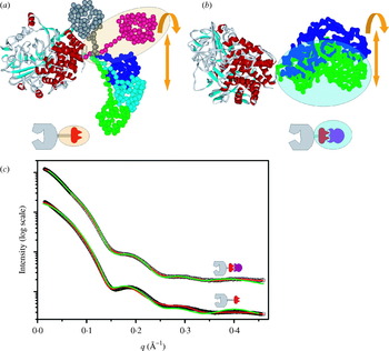
Fig. 18. Partial ab-initio models of free and complexed cellulase Cel48F. (a) Five typical CREDO (Petoukhov et al. Reference Petoukhov, Eady, Brown and Svergun2002) models of linker–dockerin region of free Cel48F are displayed in different colors together superposed on the crystal structure of Cel48F catalytic domain. (b) Two restored models (green and blue) of the dockerin/cohesin complex of the complexed Cel48F using the program CREDO superposed on the crystal structure of Cel48F (PDB id 1fbw; Parsiegla et al. Reference Parsiegla, Reverbel-Leroy, Tardif, Belaich, Driguez and Haser2000). The corresponding subdomains are schematically represented below each construct. The observed displacements between individual runs of partial ab-initio restoration are highlighted with the orange arrows. (c) Experimental SAXS profiles of free (bottom curve) and complexed (upper curve) fitted by the averaged form factors of the CREDO models obtained by the program OLIGOMER (red line; Konarev et al. Reference Konarev, Volkov, Sokolova, Koch and Svergun2003), and SAXS profiles calculated from the single CREDO models (green line) (after Hammel et al. Reference Hammel, Fierobe, Czjzek, Finet and Receveur-Brechot2004a).
The biggest challenge in trying to model conformationally very flexible systems using SAXS data is to avoid overfitting the raw data. One strategy to avoid overfitting the raw data with multiple models is to leverage existing atomic structures to reduce the parameter space of the model by describing the ensemble as a set of most probable structures. To minimize potential problems with overfitting, individual conformations to be tested as probably components of the population ought to be generated independently of the SAXS data. A number of creative techniques have begun to address the problem of quantitatively modeling flexible macromolecules observed in SAXS experiments (Akiyama et al. Reference Akiyama, Fujisawa, Ishimori, Morishima and Aono2004). Various modeling approaches can be used to generate atomic models that sample conformational space for use in fitting experimental SAXS curves. Monte Carlo techniques (Buey et al. Reference Buey, Monterroso, Menendez, Diakun, Chacon, Hermoso and Diaz2007; Shell et al. Reference Shell, Putnam and Kolodner2007), exploring the dihedral space of linkers (Tai, Reference Tai2004), CONCOORD, a non-dynamical method of generating conformation sets (Schlick, Reference Schlick2001) and MD (Levy & Becker, Reference Levy and Becker2002) have all been employed.
Conventional MD methods are computationally intensive; however, several advances have increased the size of tractable conformational changes (Yuzawa et al. Reference Yuzawa, Yokochi, Hatanaka, Ogura, Kataoka, Miura, Mandiyan, Schlessinger and Inagaki2001). These new techniques include multiple time-step MD and high temperature MD (Boehm et al. Reference Boehm, Woof, Kerr and Perkins1999; Aslam & Perkins, Reference Aslam and Perkins2001; Yuzawa et al. Reference Yuzawa, Yokochi, Hatanaka, Ogura, Kataoka, Miura, Mandiyan, Schlessinger and Inagaki2001; Aslam et al. Reference Aslam, Guthridge, Hack, Quigg, Holers and Perkins2003; Hammel et al. Reference Hammel, Fierobe, Czjzek, Kurkal, Smith, Bayer, Finet and Receveur-Brechot2005; von Ossowski et al. Reference von Ossowski, Eaton, Czjzek, Perkins, Frandsen, Schulein, Panine, Henrissat and Receveur-Brechot2005; Gilbert et al. Reference Gilbert, Asokan, Holers and Perkins2006) in which simulations are run at very high temperatures (~1000 K) to prevent molecules from becoming trapped in local minima (Leach, Reference Leach and Hall2001). Similarly, many of the simulations are sped up by including only van der Waals terms and distance restraints, but not electrostatic terms (Losonczi et al. Reference Losonczi, Andrec, Fischer and Prestegard1999). Comparison of rigid-body modeling, ab-initio shape reconstruction, and reconstruction of missing domains using CREDO have given similar results to MD sampling (Marino et al. Reference Marino, Zou, Svergun, Garcia, Edlich, Simon, Wilmanns, Muhle-Goll and Mayans2006). SAXS profiles calculated using MD trajectories are particularly useful for determining the average overall shape of the minicellulosomes and for proposing plausible atomic conformations they may adopt (Fig. 19). Given the restricted amount of independent data values from SAXS experiments, the best these techniques can provide is a set of conformations that are consistent with experimental data. In the absence of additional experimental evidence, the combination of SAXS and atomic models generated by MD trajectories cannot prove the existence of any particular conformation.
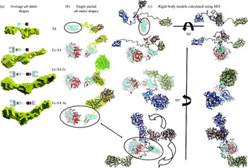
Fig. 19. The solution structure of the cellulosome. (a) The average envelope shape of different cellulosome constructs were calculated with GASBOR (Svergun et al. Reference Svergun, Petoukhov and Koch2001a). The corresponding modules are schematically represented on the top of each shape. (b) Restored partial ab-initio models of the different cellulosomes constructs calculated with CREDO (Petoukhov et al. Reference Petoukhov, Eady, Brown and Svergun2002). The CREDO models are displayed in surface representation (yellow). The fixed known atomic structures are in Cα tube representation. The secondary structural elements of superimposed atomic structures are shown as Cα tubes. (c) Best-fit models were calculated by MD of different constructs and superimposed on cohesin from S4 or complexed Cel48F (highlighted with the black circle). Three models colored by blue, brown, green for each model, except for FtS4Fc complex where only two models (green and blue) for better visualization, are presented (after Hammel et al. Reference Hammel, Fierobe, Czjzek, Kurkal, Smith, Bayer, Finet and Receveur-Brechot2005).
Once generated from atomic structures, these models can then be evaluated for their relative contribution to the scattering using SVD or the algorithm underlying OLIGOMER (Section 4.4.1). In the case of β2-glycoprotein I (β2GPI), SAXS fits poorly with the crystallized conformation or individual models with systematic modified conformations (Hammel et al. Reference Hammel, Kriechbaum, Gries, Kostner, Laggner and Prassl2002) but does fit well using a multiple model approach (Fig. 20). Not only is the inherent flexibility in β2GPI likely to be important to its function, but it also illustrates the common case in which external information must be introduced in order to generate the correct types of models to fit the observed scattering.

Fig. 20. Solution structure of β2-glycoprotein I (β2GPI). (a) The crystal structure of β2GPI (left) is shown with attached sugars (red). (b) The best single-conformation model derived from experimental SAXS data is superposed with the averaged ab-initio model calculated by program DAMMIN (Svergun, Reference Svergun, Baraberato and Koch1999) displayed as gray cages. (c) The theoretical scattering profile calculated for the mixture of different conformations improved the fit to the experimental data (root mean squared deviation for single and multiconformation fit are 3·0×10−3 and 8·5×10−3, respectively). Three different atomic conformations of β2GPI with the indicated fractional occupancies in solution are shown. Different β2GPI conformations were constructed by simple rotations between domains CCP2 and CCP3 of the best fit single structure (after Hammel et al. Reference Hammel, Kriechbaum, Gries, Kostner, Laggner and Prassl2002).
We are enthusiastic about a new approach to analyze the presence of multiple conformations of proteins contributing to the experimental scattering profile (Bernado et al. Reference Bernado, Mylonas, Petoukhov, Blackledge and Svergun2007). Bernado and co-workers define an ensemble optimization method (EOM) in which a pool of possible conformations (N>1000) is randomly generated to cover the possible conformational space. A genetic algorithm is then applied to select subsets (N=50) of configurations that fit the experimental scattering. The advantage of this method is the use of quantitative criteria for analyzing the EOM-selected models and for determining the optimal number of conformers in the subset. The best subsets are then selected for further evolution. Using both theoretical and experimental data for unstructured and multidomain proteins, EOM was able to distinguish between rigid and flexible proteins and assess interdomain contacts.
We also are enthusiastic about the potential offered by the recently developed residual dipolar coupling (RDC) NMR, which has been used to identify relative orientations in multidomain proteins relative to an external coordinate system (the ‘alignment tensor’). For multidomain proteins, the orientation of each domain can be determined separately within this coordinate frame, and the relative interdomain orientation can be deduced (Bernado et al. Reference Bernado, Blanchard, Timmins, Marion, Ruigrok and Blackledge2005). RDC data allow for unbiased determination of interdomain orientations in solution, albeit with a fourfold degeneracy, but require structural models for interpretation. In the study of the first two Ig domains of titin, Z1Z2, SAXS data was used to resolve the RDC degeneracy (Marino et al. Reference Marino, Zou, Svergun, Garcia, Edlich, Simon, Wilmanns, Muhle-Goll and Mayans2006). Calculations of the 200 RDC conformers showed that the 50 models with the lowest-discrepancy values were a well-defined cluster of conformations that superimposed with the ab-initio SAXS model, whereas the more compact crystal structure failed to fit the solution structures. Furthermore, conformational sampling using simulated averaged RDCs was applied in the analysis of SAXS profiles of partially unfolded protein. The close agreement of experimental and simulated RDC to SAXS data validated the conformational sampling results and provided a description of local structure, dynamics and average dimensions of the ensemble of unfolded protein. Thus, the synergy of SAXS with molecular modeling, crystallography, and NMR promises to provide unique insights into the structural characterization of proteins with intrinsic flexibility (Mattinen et al. Reference Mattinen, Paakkonen, Ikonen, Craven, Drakenberg, Serimaa, Waltho and Annila2002; Bax & Grishaev, Reference Bax and Grishaev2005).
4.4.3 Flexibility, oligomerization, or aggregation?
In general multidomain proteins with long linkers or that adopt extended conformations have smooth scattering profiles with few prominent features at high resolution and extended tails in P(r) functions. These proteins also typically have heterogeneous conformations with a variety of R G and D max values. Guinier plots of these macromolecules are linear over a smaller region: qR G<0·8 instead of qR G<1·3 which is more typical for globular samples (Table 1). Unfortunately, many of these features are also observed in the presence of small amounts of aggregation, which primarily affects the same low-resolutionregion of the scattering curve.
Studies on the soybean lipoxygenase-1 and rabbit 15-lipoxygenase-1 illustrate the need for careful interpretation of SAXS data in cases where flexibility is proposed (Fig. 21). The major discrepancies between the experimental scattering curve of rabbit lipoxygenase in solution and the curve calculated from the atomic coordinates were interpreted in terms of a large movement of the N-terminal domain with respect to the C-terminal domain (Hammel et al. Reference Hammel, Walther, Prassl and Kuhn2004b). Rigid-body modeling was applied, and the improvement of the fit in the entire scattering profile was observed using a mixture of different swing out conformations (Fig. 21, red, two conformations are shown; Hammel et al. Reference Hammel, Walther, Prassl and Kuhn2004b). The modeling of rabbit lipoxygenase was entirely dependent on establishing that the solution studied was monodisperse. In a study of soybean lipoxygenase, Dainese and co-workers found that the modeled structure was quite similar to the crystal structure and that slightly aggregated samples would give rise to elongated signals, as reported for rabbit lipoxygenase (Dainese et al. Reference Dainese, Sabatucci, van Zadelhoff, Angelucci, Vachette, Veldink, Agro and Maccarrone2005). Re-evaluation of rabbit lipoxygenase indicated that partial (20%) aggregation could also explain the scattering of rabbit lipoxygenase (Fig. 21).

Fig. 21. The experimental P(r) of the rabbit 15-lipoxyganase-1 (black). Theoretical P(r) calculated for a mixture of two protein conformations adopting different extensions in the N-terminal regions with the indicated occupancies (red) and for a mixture of 80% monomeric and 20% oligomeric assemblies (blue) are shown. The crystal structures used in the P(r) calculation (PDB id 1lox; Gillmor et al. Reference Gillmor, Villasenor, Fletterick, Sigal and Browner1997) using in the P(r) calculation are shown as surfaces using the same coloring (after Hammel et al. Reference Hammel, Walther, Prassl and Kuhn2004b).
Therefore, samples that are suspected of possessing intrinsic flexibility must be carefully characterized to ensure monodispersity prior to any SAXS modeling. Native gels can be very useful as an indicator of the homogeneity of samples. We have also found dynamic light scattering (DLS) useful for providing overall size and sample polydispersity measurements under the same concentrations and buffer conditions as for SAXS experiments. We have used DLS as an important pre-screening tool to optimize samples and buffers for maximum monodispersity. Our empirically based approaches to dealing with intrinsic flexibility, heterogeneous conformations, aggregation, and multidomain proteins are presented in Section 5 below.
5. Strategy and tactics for SAXS experiments
We designed and built the SIBYLS synchrotron beamline (http://www.bl1231.als.lbl.gov) at the Advanced Light Source to interconvert between a SAXS and a crystallography endstation quickly (under an hour). One of our goals in the stewardship of this beamline has been to encourage the larger community of crystallographers to use SAXS. Experience has demonstrated several pitfalls in this process. Typically crystallographers are excited about the initial results from ab-initio shape restorations only to later become disillusioned because of perceived uncertainty. In particular, some crystallographers feel that they have biased their results in a certain way. As mentioned throughout this article, in contrast to crystallography, SAXS suffers from few standardized ways of validating results. In crystallography, visibly attractive but poorly ordered crystals will immediately result in poor images in the diffraction experiment and thereby indicate data collection and processing will not be fruitful. In contrast, every solution sample gives scattering that could be processed and modeled whether or not the results are valid. Both SAXS and crystallographic analysis packages are becoming more and more like ‘black boxes’ and are frequently designed using ideal data giving few indicators about problematic data. Without a clear understanding of what information SAXS can and cannot resolve and of the metrics for judging results and the steps along the way there is a real danger of generating incorrect results from problematic data.
With increased general use of SAXS as a powerful tool to examine biological samples, it becomes necessary to have both strategic concepts and tactical plans for the assessment, processing, and interpretation of the SAXS results collected from every sample regardless of quality. Here we provide a strategic basis to proceed with data evaluation and processing for different types of data, where data-quality assessments play an essential role (Fig. 22). It is difficult to over-stress the paramount importance of collecting high-quality SAXS data, validating the level of quality by several tests, and remaining diligent in regard to possible systematic errors and other possible data problems.
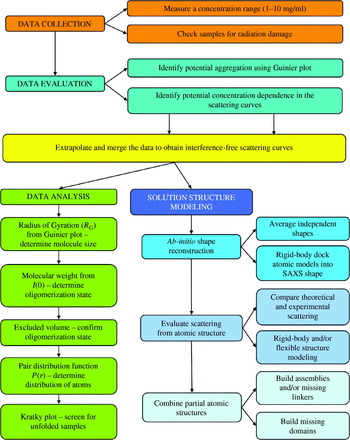
Fig. 22. Schematic for SAXS data collection, evaluation, analysis, modeling, and interpretation. We favor the combination of atomic structures with SAXS envelope modeling (lower right) where possible. Using the SAXS experimental observations identifies possible flexibility along with shape, assembly and conformation in solution.
Based upon our experience with many types of samples, we recommend the strategy and tactics shown schematically in Figs 22–25. Conceptually the SAXS experiment can be divided into four major steps: data collection, data evaluation (Fig. 23), data analyses (Fig. 24), and solution structure modeling (Fig. 25), each of which is detailed below.
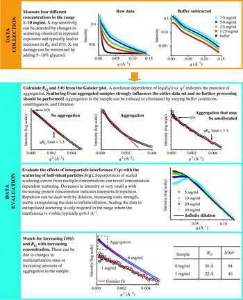
Fig. 23. Data collection and evaluation.
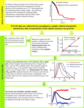
Fig. 24. Data extrapolation, merging, and analysis. Proper data analysis as outlined is essential to any further modeling and interpretation.
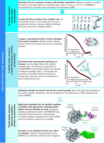
Fig. 25. Solution structure modeling and interpretation.
5.1 Data collection
At the SIBYLS beamline, 15 μl of a well-behaved 100 kDa protein in typical buffers can provide SAXS data with noise levels below 1% out to q=0·3 Å−1 at a wavelength of 1 Å in a 30-s exposure. As described below collecting data as a function of concentration is an important quality control in SAXS analysis and four concentrations between 10 and 1 mg/ml at the same volume are recommended. A minimum amount of sample for the same protein for interpretable data under the same conditions is 15 μl at 1 mg/ml. Typical data collection times are 1–100 s although millisecond time-resolved experiments are possible.
A number of parameters affect the amount of sample required for data collection. The difference in average electron density between the sample and bulk solvent plays a key role. For example, RNA and DNA, which have greater scattering contrasts than protein, require lower sample concentrations for equivalent signals (Fig. 26). Similarly, osmolites in buffers can decrease the scattering contrast with macromolecules. Salt concentrations, particularly above 1 m NaCl, will require higher sample concentrations than low salt buffers for equivalent signals. Detergents, which are commonly used for stabilizing and purifying hydrophobic molecules, can also be problematic, as detergent micelles scatter very well. Collecting data at detergent concentrations below the critical micelle concentration is required for most standard analysis. Similarly, macromolecular size is also very important. The total scattering from the same mg/ml concentrations of a small macromolecule is equivalent to that of a larger macromolecule; however, the angular distribution of scattering is not the same. At the same mg/ml concentration, larger macromolecules have stronger scattering in smaller q-ranges than smaller macromolecules. If small angle information is desired from larger macromolecules for determination of mass, R G, D max, and aggregation, lower sample concentrations will be required. The amount of sample required also varies with incident beam size, wavelength and whether static or flow cells are used.

Fig. 26. SAXS from RNA samples. (a) Experimental scattering curves of SAM-riboswitch at 1 mg/ml (red) and a 95-bp RNA molecule at 0·7 mg/ml (courtesy of Robert Rambo) in comparison to lysozyme 2·5 mg/ml (gray). For better comparison the curves have been normalized by concentration and molecular weight. (b) The calculated P(r) functions for the samples shown in panel (a) are shown with the maximum value normalized to 1. (c) Average ab-initio model of the SAM-riboswitch (red) superposed on the theoretical dimer of the crystal structure (PDB id 2gis; Montange & Batey, Reference Montange and Batey2006) (green and cyan). Average ab-initio model of the 95-bp RNA (blue wireframe) superposed on single DAMMIN model of (blue beads). The beads models reconstructed with DAMMIN (Svergun, Reference Svergun1999) were transformed into wireframe model using SITUS (Wriggers et al. Reference Wriggers, Milligan and McCammon1999).
Many SAXS instruments can adjust the q-range over which data may be collected in one single exposure. This may be done by adjusting the sample to detector distance, the incident wavelength, or the offset of the detector relative to the direct beam. Changing the q-range can require a prohibitive amount of time and one stable and well-calibrated configuration is often required.
Properly choosing beamline geometries to collect the appropriate scattering information is important. The first consideration is to capture the q-range necessary to accurately determine values for both R G and D max while obtaining sufficient information for being able to use the data for structural modeling purposes (Fig. 23). In theory the minimum q necessary for determining R G is q min⩽π/D max; however, for determining R G from Guinier plots (Section 2.3.2), multiple points are required and the linear region (q minR G<1·3 for globular samples and q minR G<0·8 for elongated samples) can be more constrictive than the theoretical constraints. For large complexes, getting sufficiently low q data by increasing the sample-to-detector distance or decreasing the incident X-ray wavelength may be required. For example, the small well-folded maltose-binding protein with R G=22·1 Å and D max=52·0 Å, requires a q min of <0·059 Å−1, which is readily achievable in most default SAXS station geometries, whereas the E. coli MutS tetramer has a R G=80·8 Å and D max=250·0 Å and requires a minimum q of <0·013 Å−1 (Mendillo et al. Reference Mendillo, Putnam and Kolodner2007), which may require more careful experimental setup. In contrast, in order to sufficiently constrain D max, a maximum q of q max⩾2π/D max is required. For large complexes, such as the MutS tetramer, this required limit q max⩾0·025 Å−1 is typically not a problem for normal geometries; however, for small proteins this limit should be checked.
Larger q values inherently provide more information and give structural reconstruction algorithms more information to fit which helps constrain the resulting solutions (Fig. 23). Unfortunately, since scattering intensity falls off rapidly, higher concentrations (which may not be possible) and/or longer exposures may be required for adequate signal to noise in the high q region. While high q data can be very valuable, especially for particle reconstruction, care should be taken so as not to sacrifice accurate low q data for extremely noisy high q data, especially in the case of X-ray sensitive samples.
Much like UV spectroscopy, the scattering from the buffer must be subtracted from the sample. There are several technical challenges in the subtraction for SAXS. First, the signal in SAXS data lies very close (typically within a few degrees) of the incident beam. In order to measure the data, the sample to detector distance is typically on the order of a meter, and the incident X-ray beam must be tightly collimated and focused and carefully blocked, as it typically has 1010-fold higher intensity than the scattered X-rays. Stray rays of the primary beam can dominate the scattering. Often some portion of these stray rays are present during data collection but can be subtracted with the buffer. Second, small buffer differences, even a micromolar difference of salt concentration, can cause large differences relative to signal at high resolutions. Thus, the sample is typically exchanged into the buffer that is used as a blank prior to the experiment by dialysis or size-exclusion chromatography. Third, to avoid systematic errors due to small differences in X-ray path lengths, the samples and blanks are measured in the same cuvette, which has windows made of a material that scatters X-rays poorly, such as mica, kapton, or beryllium. Fourth, the fact that the identical cuvette is used for the sample and blank prevents them from being measured simultaneously. Even at relatively stable synchrotron X-ray sources, changes in the intensity of the X-ray beam can easily be larger than 10−3 or 10−4 over the time-frames in which samples are measured and the cuvette is washed. Thus, the resulting scattering must be normalized by the intensity of the incident X-rays. Fifth, correction for the difference in X-ray absorption by the sample and the buffer can be applied, although the correction is small and is commonly ignored.
One of the first quality checks that must be performed during data collection is to determine the sensitivity of the sample to X-ray irradiation damage. Changes between SAXS profiles collected by multiple short exposures can indicate radiation sensitivity. Additionally, samples with radiation damage tend to aggregate, showing increasing R G and I(0) as a function of total X-ray exposure. We also routinely check samples before and after longer exposures even for samples that pass initial screening of radiation sensitivity. Several options exist to deal with samples that have inherent radiation sensitivity. Cooling the sample, diluting the sample, and adding free radical scavenging compounds or protectants like glycerol have helped prevent aggregation (Kuwamoto et al. Reference Kuwamoto, Akiyama and Fujisawa2004). Flow cells can also significantly improve data collection for very sensitive samples, although flow cells can require much more material. Alternatively, data from multiple short exposures can be summed where each exposure is performed on a fresh sample.
For samples without radiation damage, individual frames can be averaged. Background/buffer scattering should be measured both before and after the measurement of the sample. Scattering due to macromolecules is then calculated by subtracting the buffer blanks from the sample. The resulting scattering curve calculated using buffer blanks measured both before and after the sample should be identical. Data collected from several types of SAXS set-ups require ‘de-smearing’ due to incident beam properties. This is not required for sources with point focusing at the detector.
5.2 Data evaluation
One of the attractive features about SAXS data collection is that data evaluation can be performed during data collection. This is particularly useful with limited time and/or material. For example if samples shows signs of aggregation at an intermediate concentration, higher concentration measurements are unlikely to be fruitful (Fig. 23). A better use of the available material might be to dilute the concentrated samples into different buffers to screen for conditions that give better scattering.
Often the first parameter extracted from data evaluation is R G (Table 1), which can be determined from the slope in a Guinier plot [log(I(q)) vs. q 2] (Fig. 23). A Guinier plot can be easily generated from the raw data using the program PRIMUS. Nonlinear behavior in the Guinier plot in the range q<1·3/R G indicates the presence of aggregation. The scattering from the aggregation influences the entire dataset and any further data processing should proceed with caution. Some samples may show nonlinearity over a small region within the Guinier region and the remaining data is linear. Data clipped at the lowest q values where aggregation is most apparent may be processed further. However, when possible, varying buffer conditions, centrifugation and filtration should be attempted to remove the aggregation for further analysis as the aggregation may have subtle effects throughout the scattering profile (Fig. 27).
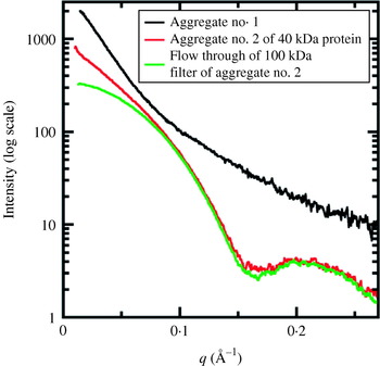
Fig. 27. Characteristic scattering of aggregates in SAXS. A fully aggregated sample is shown in black. This aggregate has no features in the scattering curve and indicates a poorly behaved sample. Lack of features in the scattering curve can also be observed with unfolded samples. Unfolded and aggregated samples can be distinguished using a Kratky plot. A partially aggregated sample is shown in red. In this scattering curve, only the lowest resolution scattering is affected, and this type of scatter can be observed both through the low-resolution shape of the scattering and disagreement between I(0) and R G calculated from the Guinier plot and from the P(r) function by indirect Fourier transformation. Passage of the sample through a filter with a 100 kDa cut-off removes the aggregated material and allows an aggregation-free scattering curve to be collected (green line).
With ideal samples, scattering profiles from a concentration gradient should be superimposable when scaled by concentration. In this case individual scattering particles are not interacting with one another (Fig. 23). In some cases target macromolecules interact with one another either repulsively or attractively adding additional and unwanted correlations in solution. These correlations affect the scattering profile, usually in the lowest resolution region (q<0·1 Å−1). For example, decreasing intensity at very small q with increasing protein concentration indicates the presence of repulsion forces. In these cases, the observed scattering is treated as a product of the scattering curve of the particle in ideal solution (the ‘form factor’ of the particle) and interactions between particles (the ‘structure factor’ of the solution). An interference-free scattering due to the ‘form factor’ can then be extracted by measuring at least three different concentrations. Lowering the concentration increases the average distance between particles and decreases the strength and effects of interparticle interactions. Thus, these curves can be used to extrapolate the scattering to infinite dilution. Long-range interactions can also be removed or diminished experimentally by changing the buffer, such as by screening electrostatic interactions by increasing salt concentration.
5.3 Data analysis
For SAXS data that is free of aggregation, radiation damage, and long-range interactions, data analysis may proceed (Fig. 24). Determination of the experimental parameters R G, I(0), D max, excluded volume, and molecular weight is the first step in reconstruction of the solution structure (Table 1). R G and I(0) can be determined from the SAXS curve using the Guinier plot or through calculation of the pair-distribution function, P(r) (Section 2.3.3; Table 1, Fig. 24). Disagreement between the values may be a sign of improper assignment of D max for the indirect Fourier transformation or other problems such as heterogeneity or unfolding.
Extended and globular macromolecules can be distinguished by P(r), as globular particles have bell-shaped functions, whereas extended particles have functions with a maximum at short distances and a long extended tail (Figs 5 and 10). Unfolded samples not only have P(r) functions consistent with extended molecules, they also possess characteristic Kratky plots [I(q)q 2vs. q] lacking bell-shaped peaks and having a plateau or a slowly increasing curve at large q values (Section 2.3.2, Fig. 24). For proteins, if R G is substantially larger than the theoretical value for a globular protein of the same molecular weight then the protein is likely in an extended conformation or potentially an oligomer (Fig. 24). The theoretical R G can be calculated by:
Determining the oligomeric state requires a determination of molecular weight, such as methods relying upon I(0) (Section 2.3.5). Most often the monomeric molecular weight is known and non-integral stoichiometries from I(0) imply heterogeneous multimerization. The excluded volume calculated through the Porod invariant can be converted to a mass (Table 1; Section 2.3.5). For proteins, a rule of thumb is to estimate the mass by dividing the excluded volume derived this way by 2. This accounts for the hydration layer as well as the protein volume. This estimate holds up well for large globular proteins (>70 kDa) but fails for proteins with unusual shapes and is particularly problematic for small proteins.
5.4 Structure modeling and interpretation
If a solution of folded macromolecules is monodisperse, then the measured scattering profiles can be used for solution structure determination (Fig. 25). Ab-initio shape determination can be applied to reconstruct the low-resolution envelopes of the protein if atomic structures are not available (Section 4.3). For this purpose programs DAMMIN, DALAI_GA, SAXS3D, or GA_STRUCT can be used. If the number of residues of the protein is known, the program GASBOR has the advantages of providing significantly more sophisticated penalties that constrain the models and of not prohibiting the generation of cavities and other anisotropic shapes (Svergun et al. Reference Svergun, Petoukhov and Koch2001b). Comparison of multiple reconstructions is extremely important to verify the stability of the solution. Multiple repetition of the modeling process significantly decreases the risk of inferring erroneous shapes. The program DAMMAVER aligns, averages, checks the uniformity, and computes a probability map of the given ab-initio models.
Ab-initio shape restoration programs allow further constraint on the solution by enforcing known symmetry. Ab-initio shape-determining programs are known to provide accurate solutions given the correct symmetry (Table 4, Fig. 25). In fact, correctly enforced higher symmetry improves the resolution of final models. Unfortunately given incorrect symmetries ab-initio programs will often find shapes that also fit the scattering profiles. Assuming higher symmetry with knowledge of only the molecular weight must be carefully justified. Identification of the fourfold symmetry of the potassium channel by comparing NSD and χ2 values derived from the SAXS data alone (Fig. 16) may not be generally applicable, especially for less anisotropic assemblies.
If the atomic structure of the sample is known or an atomic model has been proposed, comparison of theoretical SAXS profile with the experimental data is the first step in the structure evaluation (Fig. 25). The theoretical SAXS profile can be calculated with the program CRYSOL, using the χ2 agreement to evaluate the best models. Agreement between theoretical SAXS curves from crystal structures and experimental SAXS data of χ2<3·0 are not uncommon. Ab-initio shapes and atomic resolution models may be superimposed by using the programs SUPCOMB or SITUS.
One possible reason for disagreement between atomic resolution models and SAXS results is the presence of heterogeneous multimerization. This may be apparent if the molecular weight is determined. Nevertheless the program OLIGOMER can take the calculated scattering profiles of several proposed multimers and determine the fractional concentration of each multimer required to best fit the data. An excellent fit with OLIGOMER and a poor fit with CRYSOL implies heterogeneous multimerization. Other possibilities for disagreement between models and SAXS data are flexibility and truncated loops (common in crystal structures where disordered regions are not built into models). Generating a variety of conformations of the flexible regions and using OLIGOMER may improve the final fit.
If the sample is a multimeric assembly and atomic models of all subunits are available but arrangement is unknown, then rigid-body modeling can be applied (Table 2, Fig. 25). Quaternary structure modeling of a complex against the SAXS data can be performed manually using the program MASSHA or fully automatically using program SASREF. If the full-length protein represents an assembly of the domains connected by linker regions, a combination of rigid-body modeling of the subdomains and ab-initio modeling of the missed linker using flexible chains of interconnected residues can be applied. The program BUNCH allows determination of three-dimensional structures of multidomain assemblies based on multiple scattering data sets from deletion mutants when the structure(s) of individual domains are available. Other conformational sampling methods can be applied (Table 3, Fig. 25) to model the quaternary structure of multidomain assemblies. Final models are evaluated in terms of the goodness of the fit of their calculated scattering curves to the experimental data. Comparison of models generated from rigid-body modeling and ab-initio shape restorations are also very useful in establishing the validity of the results (Fig. 25).
5.5 Criteria for evaluation of SAXS results
In preparing or evaluating publications with SAXS results, measurements and analyses it is critical to have metrics identifying the reliability of extracted information. In the long term, establishing standards for SAXS data analyses will be important for judging accurate SAXS measurements and modeling, and for the larger community in the interpretation and publication of SAXS data. Whereas universally accepted quality control parameters for SAXS results comparable to those currently used for crystallography do not yet exist, we suggest here some empirical criteria to consider for SAXS data-quality control and to help avoid over-interpreting SAXS results (Table 5). We propose this information should be presented in studies concerned with SAXS solution structure modeling of biological macromolecules.
Table 5. SAXS parameters for data validation and interpretation

The first crucial parameters for SAXS data validation comes from the linearity of the Guinier plot and R G value calculated from this plot (Figs 23, 24). Ideally the concentration dependence of the R G value should be presented and a corrected R G value calculated if necessary (Section 5.2). The P(r) function and derived D max value provide a second set of important parameters. If the P(r) function gives an extremely elongated tail, accurate characterization of D max may not be possible and a possible symptom of heterogeneity (Fig. 24). Further structural interpretation of these SAXS data may be suspect. D max can be validated by calculating the P(r) function in the larger r range where r max is greater than the expected D max and/or by calculating the P(r) function without the constraints that enforce P(D max)=0 (Section 2.3.3). I(0) and R G may also be calculated from the P(r) function and should correspond to those derived from the Guinier plot.
Molecular weight determination using I(0) is directly related to the excluded volume, and if SAXS is used to determine the oligomerization state, then accurate calibration of I(0) is necessary (Section 2.3.5, Fig. 24). These calibrations are particularly useful in identifying sub-stoichiometric amounts of aggregation or mixed assembly states that need to be analyzed and modeled as mixed populations and not homogenous samples that can be easily used for low-resolution structure reconstruction.
In solution structure modeling from SAXS measurements, it is important not only to validate the fit of the calculated to the experimental SAXS data using R or χ2, but also to compare multiple modeling runs (Fig. 25). Multiple trials of the modeling process significantly decrease the risk of over interpretation of underdetermined models. We suggest that at least 10 repetitions are required to obtain an accurate average model for evaluation. Probably the easiest way to validate differences in the models is to use a NSD parameter to validate the stability and convergence of the multiple modeling rounds (Section 4.3). For cases where rigid-body refinement is used, comparisons of R G, D max, and the P(r) functions of the models to the experimentally determined values can also provide substantial insight into the quality of the model as well as the differences between any pseudo-atomic model and the experimentally observed scattering (Sections 4.2.4, 4.2.5). Handedness cannot be resolved using SAXS structures alone. Conclusions where chirality is important should be carefully examined.
5.6 Accuracy and resolution of SAXS experiments, measurements, and models
A critical issue for both SAXS and crystallography is defining the level of accuracy of resulting models. Essentially, what is the resolution of the model? For crystallography, the resolution of the structure is defined as the resolution of the data used to determine the structure. Robust quantitative measures are used to define the resolution of the resulting structure, even if the exact values of some criteria are debated. For example, a common set of criteria to define a 2 Å resolution crystal structure would expect over 50% of the data with Bragg spacings of 2 Å to be measured with a signal-to-noise ratio of more than 2 and good agreement between multiply observed reflections (R sym≪50%).
A SAXS resolution per se is more difficult to define, as there are two different types of resolution that need to be addressed: (1) the nominal resolution of the experimental scattering curve, and (2) the effective resolution of the model. The nominal resolution of the experimental scattering curve can described in a manner related to that of crystallography. The relationship between q and Bragg spacing (d) is d=λ/(2 sin(θ))=2π/q. Thus, q min sets the largest dimensions observable in an experiment (q min=0·006 Å−1 or d=1000 Å is often possible). The limiting experimental factor is how close reliable data can be determined near the primary beam. Similarly, q max sets the smallest Bragg spacing observable in an experiment (q max=0·6 Å−1 or d=10 Å is often possible). The limiting experimental consideration is the noise in the experimental data. At Bragg spacings smaller than 10 Å, the signal due to organization of bulk solvent begins to overpower the signal from the relatively small population of solutes (Head-Gordon & Hura, Reference Head-Gordon and Hura2002), as the difference between the buffer solution and protein solution becomes very small at larger values of q.
The resolution of models derived from SAXS reconstructions is frequently not described in the literature, and models are simply termed ‘low-resolution’ structures. Part of the difficulty in determining the resolution of SAXS envelopes or SAXS-based models arises from the fact that fitting of the SAXS curve does not provide a unique solution, particularly for ab-initio envelopes. Averaging is needed to construct a reasonable model for the observed scattering. The resolution of the final averaged model depends both on reciprocal resolution defined by measured q-range and data quality, as well as on the molecular size, shape, and flexibility (Section 4.3.1). For example, averaging of different models can eliminate higher resolution details, particularly if molecules are flexible such as shown in Fig. 9. The single ab-initio model (orange beads) matches the experimental data to highest resolution 13 Å (q max=0·47 Å−1); however, the model's structural details do not reach this spatial resolution, and the averaged model (blue transparent beads) is at an even lower resolution. Alternately, more details can be visualized through the incorporation of atomic-resolution models in conjunction with SAXS data (Fig. 9), and can allow details of the model to more closely match the experimental resolution, which can be critical for determining different types of structural details (Fig. 28). In general, if the synchrotron-based high-angle scattering is combined with crystal structure even the dynamic aspects of reaction-linked changes in protein conformation can be quantitatively monitored (Tiede et al. Reference Tiede, Zhang and Seifert2002). Thus in a well-defined SAXS experiment, the effective resolution can be impressive and certainly sufficient to address questions of conformational state (Davies et al. Reference Davies, Tsuruta, May and Weis2005; Chen et al. Reference Chen, Doucleff, Wemmer, De Carlo, Huang, Nogales, Hoover, Kondrashkina, Guo and Nixon2007; Yamagata & Tainer, Reference Yamagata and Tainer2007), see for example Fig. 17. In contrast, flexible multi-domain systems will show broad variations from the averaged structures but can be improved by introducing atomic models (Fig. 19).
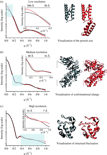
Fig. 28. The resolution range required to identify structural features in SAXS data is qualitatively illustrated showing the theoretical X-ray profile calculated by CRYSOL (Svergun et al. Reference Svergun, Baraberato and Koch1995) for proteins with A. different oligomerization states, B. different domain conformations and C. different structural fluctuations. The resolution ranges are highlighted with blue box and the upper axis of the inset graphs indicate the spatial resolution (![]() =2π/q) of this range. (a) The low angle scattering information (500–30 Å resolution) is determined particle size and overall shape, as illustrated by a monomeric (black) and dimeric (red) assemblies of the extracellular fibrinogen-binding protein (PDB id 2gom; Hammel et al. Reference Hammel, Sfyroera, Ricklin, Magotti, Lambris and Geisbrecht2007). (b) The medium angle scattering (40–16 Å resolution) provides information about domain motions, as illustrated by the scattering profiles of human glucokinase without (black; PDB id 1v4s) and with (red) a glucose analog (PDB id 1v4t; Kamata et al. Reference Kamata, Mitsuya, Nishimura, Eiki and Nagata2004). (c) The high angle scattering information (16–7 Å resolution) provides information about small structural fluctuations, as illustrated using the different conformations of the oxidized horse heart cytochrome c determined by crystallography (black; PDB id 1cr; Sanishvili et al. Reference Sanishvili, Volz, Westbrook and Margoliash1995) and NMR (red; PDB id 1akk; Banci et al. Reference Banci, Bertini, Gray, Luchinat, Reddig, Rosato and Turano1997).
=2π/q) of this range. (a) The low angle scattering information (500–30 Å resolution) is determined particle size and overall shape, as illustrated by a monomeric (black) and dimeric (red) assemblies of the extracellular fibrinogen-binding protein (PDB id 2gom; Hammel et al. Reference Hammel, Sfyroera, Ricklin, Magotti, Lambris and Geisbrecht2007). (b) The medium angle scattering (40–16 Å resolution) provides information about domain motions, as illustrated by the scattering profiles of human glucokinase without (black; PDB id 1v4s) and with (red) a glucose analog (PDB id 1v4t; Kamata et al. Reference Kamata, Mitsuya, Nishimura, Eiki and Nagata2004). (c) The high angle scattering information (16–7 Å resolution) provides information about small structural fluctuations, as illustrated using the different conformations of the oxidized horse heart cytochrome c determined by crystallography (black; PDB id 1cr; Sanishvili et al. Reference Sanishvili, Volz, Westbrook and Margoliash1995) and NMR (red; PDB id 1akk; Banci et al. Reference Banci, Bertini, Gray, Luchinat, Reddig, Rosato and Turano1997).
Although the nominal experimental resolution sets a limit on the maximum possible resolution for the SAXS model, the resolution of the data does not define the effective resolution of the model. Determining the effective resolution is more difficult and has strong similarities for the determination of the resolution of models derived from EM. In EM, resolution is estimated by the Fourier shell method, which indicates the highest resolution shells that show agreement in reciprocal space for two independently processed sets of data. This assumes coherence in Fourier space and random Gaussian error in electron density maps. In principle, this method could be used for SAXS, but validation of this approach is currently a research problem, as the degree of systematic error is not as well defined as it is for EM or crystallography. In NMR, structures are not defined as having any particular resolution, but are rather given a confidence level equivalent by the root-mean-squared derivation from the averaged structure. A SAXS equivalent would be to examine the variance of the single model volume from the averaged volume envelope. As we favor the use of high-resolution structures as restraints in the SAXS experiments, another approach would be to define the variability of a fit of known domain structures into the SAXS envelope. This would be analogous to the accurate correlation-based approaches used for EM, where the solution sets are used to define confidence intervals and error margins for the fitting parameters (Volkmann & Hanein, Reference Volkmann and Hanein2003). The definition of valid and robust measures of resolution will be important advance for SAXS experiments. A true measure of resolution will allow researchers know whether to trust or ignore the finer features of SAXS shapes and conformational changes as well as enable them to identify to what extent additional runs of shape modeling programs will enhance their final model. We recommend that publications of SAXS models make explicit the sources of error, intended level of accuracy, and estimated model resolution with the bases for the estimates stated. Ab-initio SAXS-based models should be used for experimental design or in combination with other types of information, as they are generally not sufficiently over determined by the SAXS experiment alone.
We note that the resolution required in any experiment depends upon the biological question of interest. The lower resolution diffraction from B-form DNA turned out to be more useful than the higher resolution A-form DNA diffraction for defining the structure of the double helix (Franklin & Gosling, Reference Franklin and Gosling1953a, Reference Franklin and Goslingb). In cases involving conformational flexibility and transitions, lower resolution results that can be used to describe the flexibility can potentially answer biological questions of interest better than high-resolution experiments that enforce a single conformation. In general, the great strength of SAXS experiments is that they characterize the overall molecular shape and assembly in solution, and delineate the architectural arrangements needed to place high-resolution structures of components. This is precisely why the combination of SAXS with a high-resolution method such as crystallography becomes so powerful.
6. Prospects and conclusions
6.1 General biological and biophysical implications
The use of both X-ray crystallography and SAXS is poised to be tremendously relevant for addressing the different biological pathways that control cells and offers enormous potential impacts in areas ranging from bio-energy to medicine. The current initiatives in genome sequencing along with the resulting whole-genome bioinformatics studies have revealed that not only are the components of signaling pathways modular (Bahattacharyya et al. Reference Bahattacharyya, Remenyi, Yeh and Lim2006), but so are the proteins that make them up (Apic et al. Reference Apic, Gough and Teichmann2001). These modular architectures within complexes and within individual proteins allow independent activities to be functionally coordinated. At the extreme, there are important proteins playing dynamic roles where interactions between multiple partners are exchanged to coordinate important cellular processes. Dynamic interactions within cells may be important in several respects: (1) to increase recognition probability, via significantly enlarging the area and three-dimensional size of the target, (2) to reduce disruptive interference among macromolecular steps and pathways, (3) to create highly effective local concentrations of components at target sites, (4) to promote pathway coordination, and (5) to allow a degree of self-regulation.
Biophysical studies have indicated that macromolecular complexes are formed through local contacts dominated by short-range interactions at the binding surface. Shape and chemical complementarity are critical features that control the mechanisms of assembly. Thus, the control of interface shape provides simple structure-based mechanisms to control cellular processes. Moreover, these studies also predict the existence of molecules that are primarily required as molecular scaffolds and jigs that bring together appropriate active components within complexes and may possess substantial flexibility. In some cases these scaffolding molecules and domains are dispensable with the introduction of appropriate fusions. For example, telomeres can be properly maintained when Cdc13 and Stn1 are replaced with a fusion of the Cdc13 DNA binding domain onto Stn1 (Pennock et al. Reference Pennock, Buckley and Lundblad2001). Similarly, a Cdc13-Est2 fusion protein eliminates the requirement for the Est1 protein for telomerase function (Evans & Lundblad, Reference Evans and Lundblad1999). The presence of these scaffolding domains and proteins in normal cells, however, provides the opportunity for additional cellular levels of control. For example, fusion of the Sld3 and Dpb11 proteins bypasses the requirement for the phosphorylation of Sld3 by the budding yeast cyclin-dependent kinase and the phospho-binding BRCT domains of Dpb11 (Zegerman & Diffley, Reference Zegerman and Diffley2007). However, this fusion comes at the cost of the regulation that the cyclin-dependent kinase normally performs in coordinating the yeast cell cycle (reviewed in Mendenhall & Hodge, Reference Mendenhall and Hodge1998). Understanding these types of mechanisms in the context of the native systems will require structural characterization of the various conformational states these proteins adopt, regardless of whether or not a particular molecule or conformational state is suitable for high-resolution structural studies.
Decision-making by biological pathways involves dynamic molecular interactions. These interactions are pathway specific and can include the formation of cooperative ensembles, use of interface mimicry and exchange, switching of states in chemo-mechanical assemblies, and flexing by unstructured regions. Studying these processes by any single biophysical technique can be remarkably challenging. Thus, many of these systems are ideal targets for the combination of SAXS with high-resolution structures and computational techniques.
6.2 Needs and prospects
Combining data from solution scattering with atomic resolution structures holds tremendous promise for addressing biophysical details of how specific complexes and flexibility drive biological processes. The challenge has been that this combination requires understanding of biology, structures, solution scattering, and computational methods. Thus, the goal of this review has been to introduce sufficient detail for each of these techniques so that they can be productively applied in the context of this problem. We note that advances continue to be made in each of these fields, and we predict that several areas in SAXS data collection and processing are positioned to become important developments in the near future.
One issue that would benefit from sustained theoretical and practical study is the development of a universally accepted SAXS assessment factor or factors that are equivalent to the R-factor in crystallography. One of the fundamental requirements in the modeling is to be able to successfully measure the fit of proposed models to solution scattering curves. As detailed in Section 4.1, we do not consider this to be a solved problem, and we expect that multiple measures might be required depending on the types of modeling that are performed. An equally important statistical measure for evaluating this fitting is an equivalent to the crystallographic R free. However, a perfect analog is unlikely, as the limited number of independent parameters measured in a SAXS experiment make it unwise to extract a sufficient number for use as an unrefined reference set.
Additionally, we believe that efforts to automate SAXS data collection and processing will be profoundly important. The requirement of using the same cuvette for buffers and samples typically means that cuvette washing and filling take up a substantial fraction of the synchrotron time allocate for experiments. Thus, the use of flow cells, robotics, and temperature-controlled sample holders offer the possibility of streamlining the SAXS data collection process and can allow for rapid screening of many conditions. These can include different buffer conditions to control aggregation, titration conditions to understand specific conformational changes, or small molecules from libraries to search for lead compounds that inhibit or promote complex formation, control the formation of active states, or control the folding of specific targets. Similarly, the possibility of using SAXS in conjunction with an inline size-exclusion chromatography system may allow for separation and characterization of samples with dynamic heterogeneity in their assembly states. We are excited about these types of technological advances, as our experience has suggested that the ease for which experiments can be automated directly controls the type and scale of experiments that will be attempted.
We also anticipate that the use of SAXS in the study of nucleic acids, particularly RNA enzymes and riboswitches will become increasingly important, such as illustrated by glycine riboswitch (Lipfert et al. Reference Lipfert, Das, Chu, Kudaravalli, Boyd, Herschlag and Doniach2007b) and the SAM riboswitch (Fig. 26). RNA scatters X-rays approximately five times more strongly than proteins (Fang et al. Reference Fang, Littrell, Yang, Henderson, Siefert, Thiyagarajan, Pan and Sosnick2000), allowing for useful characterizations of less concentrated samples. Further, SAXS can provide helpful constraints onto the large number of potential secondary and tertiary structures that are predicted by folding algorithms such as MFOLD (Zuker et al. Reference Zuker, Mathews and Turner1999) and frequently use sequence conservation and nuclease sensitivity to be validated. RNA activity often involves conformational switching that is well defined by SAXS. SAXS allows the examination of multiple RNA states to define the active conformation, whereas the low-energy states determined in macromolecular crystallography have frequently been of inactive conformations. As SAXS provides direct measures of shape in solution, it may furthermore aid in the discovery of proteins that regulate processes by mimicry of DNA and RNA structures (Putnam et al. Reference Putnam, Shroyer, Lundquist, Mol, Arvai, Mosbaugh and Tainer1999; Putnam & Tainer, Reference Putnam and Tainer2005).
SAXS appears to offer significant potential advantages for examining the structure of membrane proteins in lipid bilayers and detergents, although this application of SAXS is still an emerging technology. The size and complexity of membrane protein complexes with detergent and lipids are major challenges to crystallization and NMR experiments, but provide potential advantages for SAXS experiments by providing enhanced contrast compared to aqueous complexes. The central challenge for SAXS is that the buffer, proteins, and lipid/detergent mixture all have different electron densities, complicating the analysis. Matching the scattering of the lipid and detergent in SAXS or SANS provides one way to address these multicomponent systems (Bu & Engelman, Reference Bu and Engelman1999). SVD has also been used to extract the scattering profile of protein-detergent complexes at concentrations above the critical micelle concentrations (Section 4.4.1; Lipfert et al. Reference Lipfert, Columbus, Chu and Doniach2007a). Embedding membrane proteins in cubic lipid phases can also control the nature of the lipid/detergent systems allowing for the generation of more closely matched blank samples (Caffrey, Reference Caffrey2000; Lunde et al. Reference Lunde, Rouhani, Facciotti and Glaeser2006). Another approach has been the use of mutant lipid-carrying proteins (Denisov et al. Reference Denisov, Grinkova, Lazarides and Sligar2004; Bayburt et al. Reference Bayburt, Grinkova and Sligar2006) to encircle the hydrophobic lipid/membrane protein complexes to form ‘nano-disks’ (Nath et al. Reference Nath, Atkins and Sligar2007). This system can potentially yield monodisperse and homogeneous particles whose size can be controlled by varying lipoprotein size; however, sample preparation and control of particle homogeneity are non-trivial challenges. While all of these current approaches will benefit from further use and development, they demonstrate the potential of SAXS to aid in the characterization of membrane proteins in lipid bilayers and detergents.
Using SAXS data as a source of experimental restraints for modeling macromolecular flexibility and computational docking is an exciting and relatively underdeveloped possibility. SAXS data from appropriate samples can provide important experimental feedback, and could be usefully extended to include dynamic conformational changes characterized by time-resolved experiments. Time-resolved measurements require very high X-ray flux and fast detectors designed for rapid electronic shuttering. Both are now available, and SAXS, unlike traditional NMR and fluorescence experiments, is not affected by the molecular rotation times, so time-resolved SAXS can be performed in an equivalent manner to the traditional static experiments. Millisecond-resolved SAXS experiments performed to date have primarily focused on following changes in R G from the highest intensity region of the scattering curve during the folding of RNAs and proteins (e.g. Kwok et al. Reference Kwok, Shcherbakova, Lamb, Park, Andresen, Smith, Brenowitz and Pollack2006; Uzawa et al. Reference Uzawa, Kimura, Ishimori, Morishima, Matsui, Ikeda-Saito, Takahashi, Akiyama and Fujisawa2006). A natural complement to the global shape and conformation from SAXS will be residue level information from advancing techniques of enhanced hydrogen/deuterium exchange mass spectrometry, which can approach single-residue resolution as shown for the photocycle changes of photoactive yellow proteins (Brudler et al. Reference Brudler, Gessner, Li, Tyndall, Getzoff and Woods2006). Thus, SAXS is well positioned to become an important player along with new weak-field aligned NMR and fluorescence experiments that can probe samples in the biologically interesting millisecond time-frame. With appropriate resources for directed efforts, SAXS can provide complementary experimental data on flexibility in macromolecular interactions with widespread impacts.
6.3 Expectations and predictions
A fundamental strength of SAXS is that it provides the overall structure including both architectural arrangements and conformations in the 50–10 Å resolution range in near physiological conditions to yield the information needed to place high-resolution structures of components in macromolecular complexes. Thus, SAXS has the potential for addressing many important issues in fundamental biology and human disease. We believe that SAXS can play an important role in identifying which of the >10 million polymorphisms identified in humans cause structural defects in macromolecules.
One major class of such disease-causing mutations is thought to cause defects in folding and structure, which can be readily observed in SAXS. Mutations in this class have already been identified to affect a number of medically relevant proteins such as the DNA repair protein BRCA1, where mutations are associated with predisposition to breast cancer, the DNA damage response protein p53, where mutations are associated with predispositions to numerous cancer types, the Werners syndrome helicase-nuclease where mutations cause rapid aging and the reactive oxygen control enzyme superoxide dismutase, where mutations are associated with neurodegenerative disease (Deng et al. Reference Deng, Hentai, Tainer, Iqbal, Cayabyab, Hung, Getzoff, Herzfeldt, Roos, Warner, Deng, Soriano, Smyth, Parge, Ahmed, Roses, Hallewell, Pericak-Vance and Siddique1993; Foster et al. Reference Foster, Coffey, Morin and Rastinejad1999; DiDonato et al. Reference DiDonato, Craig, Huff, Thayer, Cardoso, Kassmann, Lo, Bruns, Powers, Kelly, Getzoff and Tainer2003; Williams et al. Reference Williams, Chasman, Hau, Hui, Lau and Glover2003; Wu & Hickson, Reference Wu and Hickson2006; Perry et al. Reference Perry, Yannone, Holden, Hitomi, Asaithamby, Han, Cooper, Chen and Tainer2006, Reference Perry, Fan and Tainer2007). SAXS experiments provide an efficient means to ask if polymorphisms may cause structural defects as seen for the mitochondrial superoxide dismutase (Borgstahl et al. Reference Borgstahl, Parge, Hickey, Johnson, Boissinot, Hallewell, Lepock, Cabelli and Tainer1996). The ability to do rapid SAXS analyses will also allow effective use of comparative genomics experiments to distinguish different assemblies that maintain similar activities among different organisms, such as occurs for eukaryotic and microbial Cu,Zn superoxide dismutases (Bourne et al. Reference Bourne, Redford, Steinman, Lepock, Tainer and Getzoff1996). Similarly SAXS provides a basis to examine the structural conversion of the cellular prion protein into a misfolded isoform prion shape that causes human disease (Redecke et al. Reference Redecke, Bergen, Clos, Konarev, Svergun, Fittschen, Broekaert, Bruns, Georgieva, Mandelkow, Genov and Betzel2007). As SAXS has intrinsic advantages for examining both folding and shape in solution, it offers not only critical technology for characterization of such defects, but also an efficient and powerful means of drug discovery by SAXS-based screening for compounds that bind to and stabilize the native shape and assembly. SAXS offers obvious powerful advantages for identifying even low-affinity small molecule binders without requiring any labeling or the development of target specific assays. For the right problems, SAXS can be an important tool for identifying lead compounds.
A second major class of disease-causing mutations is likely to localize to macromolecular interfaces. Since these interfaces involve more residues than active site regions, more polymorphisms will likely alter interface residues. Polymorphisms that cause these surfaces to become altered or disrupted will be readily identifiable with SAXS. An important interface type involves acceptor sites that can bind multiple partners by interface mimicry and exemplified by the PCNA peptide-binding surface (Chapados et al. Reference Chapados, Hosfield, Han, Qiu, Yelent, Shen and Tainer2004; Sakurai et al. Reference Sakurai, Kitano, Yamaguchi, Hamada, Okada, Fukuda, Uchida, Ohtsuka, Morioka and Hakoshima2005; Dore et al. Reference Dore, Kilkenny, Jones, Oliver, Roe, Bell and Pearl2006; Pascal et al. Reference Pascal, Tsodikov, Hura, Song, Cotner, Classen, Tomkinson, Tainer and Ellenberger2006) or by exchange of similar interactions by multiple proteins as controlled by a third component such as DNA such as by the Rad51 polymerization interface (Shin et al. Reference Shin, Pellegrini, Daniels, Yelent, Craig, Bates, Yu, Shivji, Hitomi, Arvai, Volkmann, Tsuruta, Blundell, Venkitaraman and Tainer2003). Atomic arrangements derived from SAXS can provide additional information that can clearly resolve the altered nature of these assemblies, such as distinguishing between open trimeric versus dimeric PCNA rings that are more difficult to identify by other techniques. For example, SAXS shape predictions for PCNA accurately predicted a trimeric ring assembly while also allowing accurate prediction of the folded region of a full-length DNA repair glycosylase including structural alterations resulting from crystal contacts and truncation of a large unstructured region (Tsutakawa et al. Reference Tsutakawa, Hura, Frankel, Cooper and Tainer2007). Thus, the characterization of static and dynamic complexes by SAXS may be equally or more important than high-resolution structures of component active sites for understanding the implications of the genome project in cell biology and human health.
Results from the structural genomics initiatives provide compelling evidence for the utility of advanced SAXS technologies. These efforts indicate that about half of all eukaryotic proteins have unstructured regions of over 40 residues in length and many are at least partially unfolded without their specific protein partners. Given the ubiquity of flexibility in macromolecules, it is almost certain that deciphering the mechanistic details of biological pathways will require the integration of techniques, like SAXS. SAXS can define the overall shape, conformation, and architecture, including unstructured regions and those structures that may not adopt single states suitable for high-resolution structural studies. As more folded domain structures are being solved, the best use of available SAXS experimental information will incorporate these domains as external information, analogously to the use of residue stereochemical constraints to obtain accurate atomic models from 2·5 Å to 3·5 Å diffraction data. Similarly, for RNA and multi-domain proteins that undergo functionally important conformational changes, SAXS can test and validate active conformational states in solution. For the many membrane bound proteins that remain difficult to crystallize, SAXS provides a possible general solution to the structural characterization of membrane proteins in their hydrophobic environments with the added advantage that lipids and detergents scatter less than protein. Their contribution to the scattering may be minimized by appropriate choice of buffer. SAXS provides appropriate experimental feedback for computational modeling of conformational landscapes, docking, denatured proteins, and the folding of proteins and RNA, which should improve the accuracy of computational simulations and predictions. SAXS furthermore provides an experimental basis to identify structural similarity even in the absence of sequence homology and thereby direct efficient molecular replacement efforts for phasing crystal structure data and also validate the relevance of cross-genomic structural modeling.
SAXS is an effective and important complement to crystallography as it can provide information on every sample, faster data collection than EM or NMR, and native structural analysis in solution. Furthermore, SAXS results provide an efficient and powerful way to identify experimentally testable models for macromolecular interactions and conformations in solution. With the millions invested in crystallography to develop high-throughput structural analyses, it is tragic that SAXS, which certainly has the capacity to be a true high-throughput technique, has been neglected by comparison. The investment in SAXS is surprisingly small, as SAXS can evaluate samples and to aid in the efficient optimization of constructs for crystallography. However, given the limited funding for SAXS in the USA, it is no surprise that much of the development and software for SAXS has been accomplished in Europe and Japan. Yet, this is an exciting time in the development of SAXS and the modeling of structures using a combination of SAXS and atomic resolution structures. Much of the technological and computational infrastructure is currently in place, which substantially lowers the barriers for new experimenters to use SAXS and interpret SAXS data in their biophysical experiments. In the next decade, any funding in SAXS will more than pay for themselves in real results and substantial technological advances that address important unsolved problems in biology, medicine, nanotechnology, and biotechnology. Thus, as these SAXS tools and technologies evolve and become widely adopted, we expect that they will be applied in novel ways to not only to solve existing problems in structural biology but also to play an active role in pushing the cutting edge of research in structural biology.
Acknowledgments
We thank Betsy Goldsmith, Lorena Beese, Wei Yang, Anna-Maria Hays Putnam, Meindert Lamers, Marc Mendillo, Ken Frankel, Susan Tsutakawa, Elizabeth Getzoff, Niels Volkmann, Michael Wall, Scott Brown, Eva Nogales and Brian Chapados for comments on the manuscript. We are grateful to our collaborators and co-workers and in particular Richard Kolodner, Marc Mendillo, Scarlet Shell, Veronique Receveur Brechot, Tom Ellenberger, Hiro Tsuruta, Robert Rambo and Henri-Pierre Fierobe for contributions to the projects described. X-ray scattering and diffraction technologies and their applications to macromolecular shapes and conformations in solution at the SIBYLS beamline at Lawrence Berkeley National Laboratory are supported in part by the DOE program Integrated Diffraction Analysis Technologies (IDAT) and the DOE program Molecular Assemblies Genes and Genomics Integrated Efficiently (MAGGIE) under Contract Number DE-AC02-05CH11231 with the U.S. Department of Energy. Efforts to apply SAXS and crystallography to characterize eukaryotic pathways relevant to human cancers are supported in part by National Cancer Institute grant CA92584. J.A.T. research on flexible protein interactions and assemblies is supported in part by NIH grants AI22160, CA81967, CA104660, and GM46312. C.D.P. was funded as a Robert Black fellow by the Damon Runyon Cancer Research Foundation.


