Bipolar disorder (BD) is a fundamentally cyclical illness, not only in terms of its prototypical clinical course, characterized by alternating highs and lows of mood, energy, and behavior, but also in terms of its hypothesized neurobiological underpinnings (Abreu and Braganca, Reference Abreu and Braganca2015). Credit for first describing BD (then named, ‘folie circulaire’) as a single, fundamentally cyclical disease entity is generally given to Falret in 1851 (Falret, Reference Falret1851). Falret's conceptualization of folie circulaire was subsequently expanded on by later prominent psychiatrists, including Kraepelin with his renowned observation-based studies of ‘manic-depressive illness’ (Kraepelin, Reference Kraepelin1921), and generally dominated thinking on the matter until the 1960s, when Angst and others called for the division of manic-depressive illness into ‘unipolar’ (i.e. depression-only) and ‘bipolar’ (i.e. mania with or without depression) types based on emerging hereditability data (Angst, Reference Angst1966). This model of affective illness prioritized polarity over cyclicity, featuring unipolar v. bipolar types each defined by the lifetime occurrence of specific combinations of discrete mood episodes (DSM-III) (American Psychiatric Association, 1980), informed the development of the pre-eminent psychiatric diagnostic systems of the day that have managed to persist, largely unchanged, to the present (DSM-5) (American Psychiatric Association, 2013).
Nonetheless, since the 1980s, there has been a gradual return to Falret and Kraepelin's conceptualizations of affective illness in the BD research community (Marneros and Angst, Reference Marneros and Angst2001; Goodwin and Jamison, Reference Goodwin and Jamison2007), which focus on longitudinal course, cyclicity, and continuous ‘spectrum models,’ due to emerging supportive data (Akiskal, Reference Akiskal, Davis and Maas1983; Prisciandaro and Roberts, Reference Prisciandaro and Roberts2005; Reference Prisciandaro and Roberts2011). For example, it is now recognized that even individuals with ‘pure’ major depressive disorder (MDD) experience higher rates of subthreshold hypomania than previously recognized (Zimmermann et al., Reference Zimmermann, Bruckl, Nocon, Pfister, Lieb, Wittchen, Holsboer and Angst2009; Angst et al., Reference Angst, Cui, Swendsen, Rothen, Cravchik, Kessler and Merikangas2010, Reference Angst, Azorin, Bowden, Perugi, Vieta, Gamma and Young2011; Fiedorowicz et al., Reference Fiedorowicz, Endicott, Leon, Solomon, Keller and Coryell2011; Perugi et al., Reference Perugi, Angst, Azorin, Bowden, Mosolov, Reis, Vieta and Young2015). As a result, the characterization of mixed states and/or features was significantly modified in DSM-V compared with previous editions. Increasingly, sophisticated new longitudinal statistical methods have been developed that allow investigation of syndromal and subsyndromal mood fluctuations over the course of illness of affective disorders (Cochran et al., Reference Cochran, Mcinnis and Forger2016). The current study employed one such statistical framework, hidden Markov modeling (HMM) (MacDonald and Zucchini, Reference MacDonald and Zucchini1997), to uncover empirically derived manic and depressive symptom states from longitudinal data from the Systematic Treatment Enhancement Program for Bipolar Disorder (STEP-BD) study (Sachs et al., Reference Sachs, Thase, Otto, Bauer, Miklowitz, Wisniewski, Lavori, Lebowitz, Rudorfer, Frank, Nierenberg, Fava, Bowden, Ketter, Marangell, Calabrese, Kupfer and Rosenbaum2003), estimate participants’ probabilities of transitioning between these states over time, and evaluate whether clinical course variables and/or comorbid psychiatric disorders predict participants’ state transitions.
Materials and methods
Study overview
The design and methods of the STEP-BD study have been described in detail previously (Sachs et al., Reference Sachs, Thase, Otto, Bauer, Miklowitz, Wisniewski, Lavori, Lebowitz, Rudorfer, Frank, Nierenberg, Fava, Bowden, Ketter, Marangell, Calabrese, Kupfer and Rosenbaum2003). Briefly, STEP-BD was a multicenter naturalistic treatment study conducted at 21 US academic medical centers between 1998 and 2005 that prospectively evaluated clinical outcomes in patients with BD. Unlike most clinical trials that selectively enroll subjects in specific mood states and exclude individuals with substance abuse and other psychiatric comorbidities, STEP-BD was designed to study treatment response and clinical course in patients commonly encountered in clinical practice, regardless of current mood status, treatment regimen, or co-occurring conditions. The study allowed all participants to enter a standard care pathway in which clinic visits were scheduled as frequently as indicated and clinicians were encouraged to apply expert consensus guidelines for treatment but were free to prescribe any treatment they felt was indicated. Patients could also become eligible to voluntarily enter randomized controlled medication treatment for acute (n = 366) and refractory (n = 66) depression, or psychosocial treatment for acute depression (n = 293), but could return to the standard care pathway at any time. Over 7 years, 4360 participants aged 15 years and older who met DSM-IV criteria for bipolar I disorder, bipolar II disorder, BD not otherwise specified, cyclothymia, or schizoaffective disorder, bipolar type were enrolled in the STEP-BD study. Four thousand one hundred and eight of these participants (i.e. all participants enrolled through 30 November 2004 and scheduled for follow-up visits through 28 February 2005) were included in the publicly available STEP-BD database used for the current analyses. Of these available participants, 3918 were included in analyses because they had complete data on at least one of the dependent variables on at least one occasion. However, only 3229 participants were included in analyses involving baseline covariates, because the remaining 689 participants had missing data on at least one covariate.
Assessments
During their first year of participation, study patients completed quarterly independent assessment interviews at baseline and at months 3, 6, 9, and 12. Bipolar diagnoses and retrospective course (e.g. history of suicide attempt, history of psychosis, history of antidepressant-associated switch, past year rapid cycling, and age of BD onset) were assessed by study clinicians at baseline using the Affective Disorders Evaluation (Sachs et al., Reference Sachs, Thase, Otto, Bauer, Miklowitz, Wisniewski, Lavori, Lebowitz, Rudorfer, Frank, Nierenberg, Fava, Bowden, Ketter, Marangell, Calabrese, Kupfer and Rosenbaum2003), adapted from the mood and psychosis modules of the Structured Clinical Interview for DSM-IV; comorbid Axis I diagnoses were assessed using the Mini-International Neuropsychiatric Interview (Sheehan et al., Reference Sheehan, Lecrubier, Sheehan, Amorim, Janavs, Weiller, Hergueta, Baker and Dunbar1998). Quarterly interviews also included evaluation of manic and depressive symptoms using clinician-administered scales [i.e. the 11-item Young Mania Rating Scale (YMRS) (Young et al., Reference Young, Biggs, Ziegler and Meyer1978) and the 10-item Montgomery–Asberg Depression Rating Scale (MADRS)].
Statistical analysis
The current study used HMM (MacDonald and Zucchini, Reference MacDonald and Zucchini1997), a latent longitudinal mixture modeling approach, to uncover empirically derived manic and depressive symptom states from longitudinal data, estimate participants’ probabilities of transitioning between these states over time, and evaluate whether clinical course variables and/or comorbid psychiatric disorders predict participants’ state transitions. HMM has been prominent in recent substance use disorder research because it readily accommodates the chaotic nature of substance use in clinical studies (i.e. consistent stretches of use interspersed with unusual bursts) (Shirley et al., Reference Shirley, Small, Lynch, Maisto and Oslin2010) and reduces the impact of measurement error on parameter estimates and standard errors that originates from patients’ self-report of symptomatology. Because these methodological challenges are prominent in mood symptom reports from individuals with BD, HMM is arguably well-suited to modeling longitudinal symptom data from bipolar patients (Prisciandaro et al., Reference Prisciandaro, Desantis, Chiuzan, Brown, Brady and Tolliver2012). Additionally, unlike traditional approaches to defining the boundaries of bipolar symptom states (e.g. expert consensus and latent class analysis of cross-sectional data), typically referred to as mood ‘episodes,’ HMM identifies latent mood states using longitudinal mood symptom data.
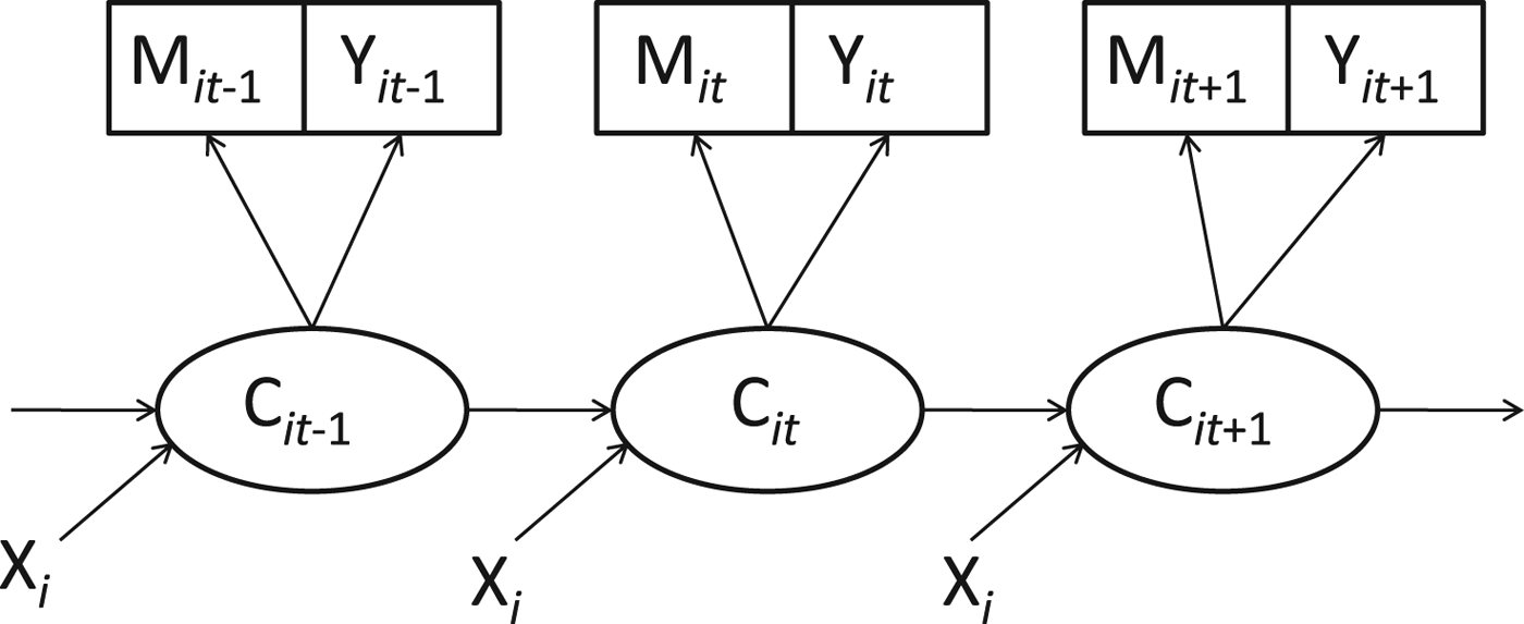
In the current study, manic and depressive symptoms, in terms of YMRS and MADRS total scores, were assumed to be manifestations of an empirically determined number of latent states, and participants were allowed to freely transit among these states across time. An optimal number of latent states was determined by comparing the relative fit [i.e. using sample-size adjusted Bayesian Information Criteria (aBIC)] (Nylund et al., Reference Nylund, Asparouhov and Muthén2007) and interpretability of several HMM models, each featuring a different number of states. To ensure that HMMs would be estimable, interpretable, and reliable, we imposed two additional constraints on selecting the optimal number of latent states: (i) the selected number of latent states, the mean of each latent state, and the probabilities of transitioning among states had to be the same for every time-point, and (ii) each state had to contain at least 5% of the sample. The probability of remaining in, or transitioning to, a given latent state from one quarter to the next was calculated from the best fitting HMM model. Finally, the best-fitting HMM model was re-estimated with covariates, selected to facilitate construct validation of the obtained symptom states, allowed to predict participants’ transition probabilities. Figure 1 presents a graphical depiction of the final estimated model (Wall and Li, Reference Wall and Li2009); M it and Y it represent the mean MADRS and YMRS scores, respectively, for participant i during study week t, C it represents the unobserved mood state of patient i at study week t, and X i represents a vector of baseline covariates (e.g. age of onset and history of suicide attempt) for patient i. All models were estimated using an estimator (Maximum Likelihood with Robust standard errors; MLR), which uses all available data and yields unbiased parameters when missing data are missing at random, in MPlus 6.1 software (Muthen and Muthen, Reference Muthen and Muthen2011); study site was included as a clustering variable for all models. Model parameterization of HMM as implemented in MPlus is described in detail in Langeheine and van de Pol (Reference Langeheine, van de Pol, Hagenaars and Mccutcheon2002; pp. 323–329) as well as the MPlus user's guide (Example 8.12) (Muthen and Muthen, Reference Muthen and Muthen2011).

Fig 1. Hidden Markov model schematic. M it and Y it represent the mean MADRS and YMRS scores, respectively, for participant i during study week t, C it represents the unobserved mood state of patient i at study week t, and X i represents a vector of baseline covariates (e.g. age of onset) for patient i.
Results
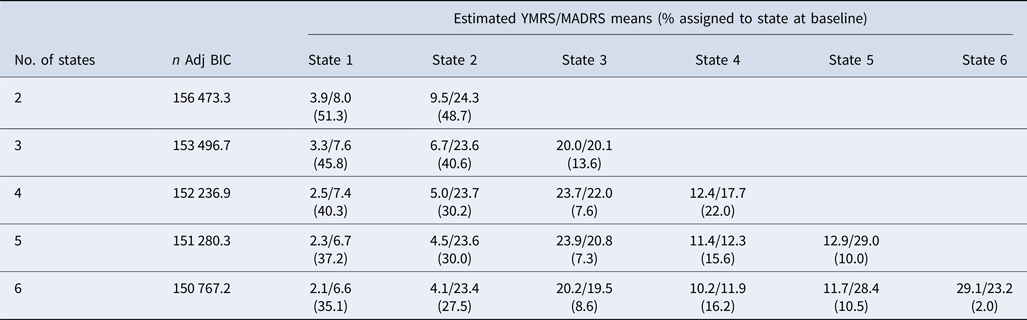
As described further below, HMM models optimally supported the existence of three latent mood states in the STEP-BD sample; baseline demographics and select clinical characteristics for the overall sample and for individuals in each of the latent states are presented in Table 1. Fit and estimated means for HMM models containing between 2 and 6 latent states are presented in Table 2. Although sample-size adjusted BIC suggested that the model with the largest estimable number of classes (i.e. 6) best fit the data, models with >3 latent states had at least one state containing <5% of the sample at some point in time. The three-state HMM consisted of ‘euthymic’ (i.e. MADRS M = 7.6, YMRS M = 3.3), ‘depressed’ (i.e. MADRS M = 23.6, YMRS M = 6.7), and ‘mixed’ (i.e. MADRS M = 20.1, YMRS M = 20.0) symptom states. Although all estimated HMM models contained ‘euthymic’ and ‘depressed’ states, additional states suggested by the four- through six-state models were further ‘mixed’ manifestations; for example, the four-state model, contained ‘euthymic’ and ‘depressed’ states, as well as two additional states with MADRS M = 22.0, YMRS M = 23.7 and MADRS M = 17.7, YMRS M = 12.4, respectively. In sum, a three-state HMM model was retained because it was maximally interpretable, fit better than an alternative two-state model, and consisted of classes that each contained ⩾5% of the sample.
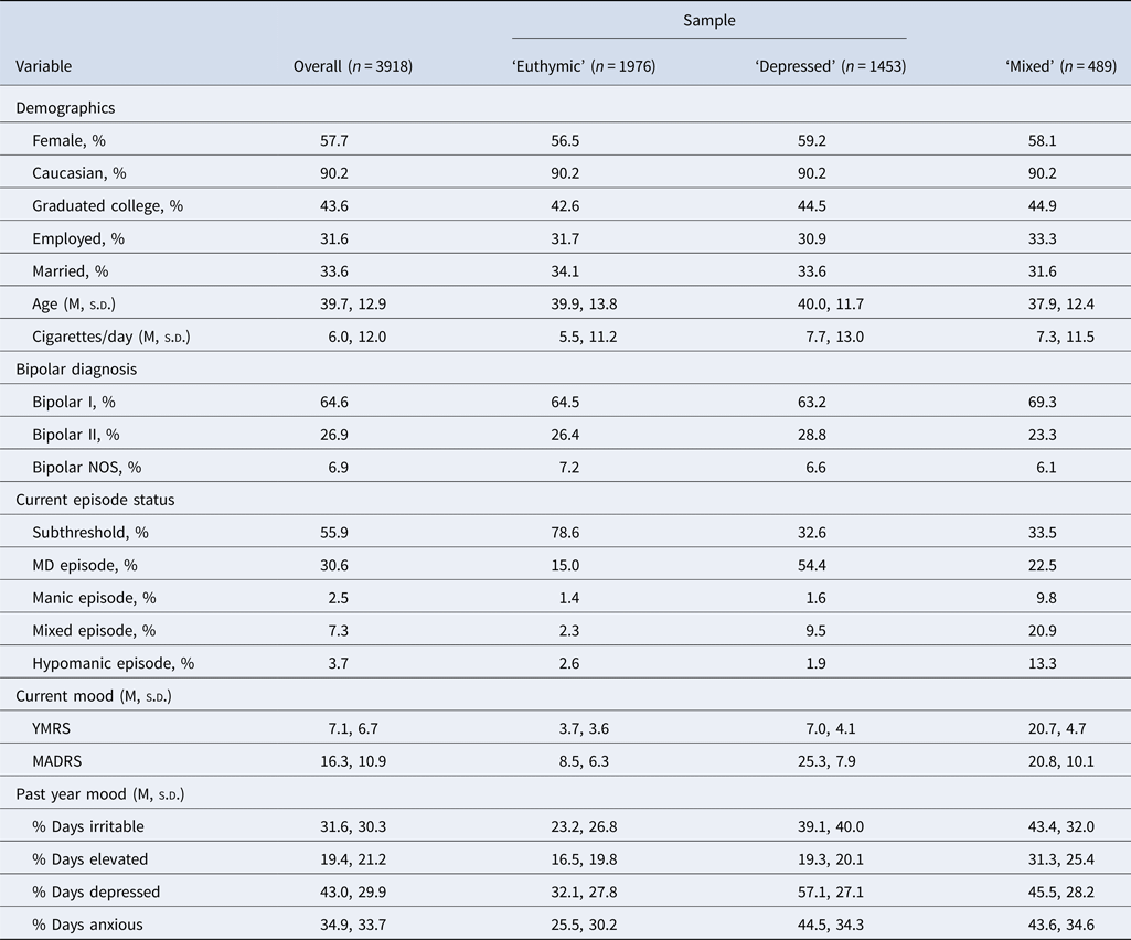
Table 1. Participant characteristics in the overall sample and by assigned latent state at baseline

NOS, not otherwise specified; subthreshold, not diagnosed with an MD, manic, mixed, or hypomanic episode; MD, major depressive; YMRS, Young Mania Rating Scale; and MADRS, Montgomery–Asberg Depression Rating Scale.
Note: Statistical tests are not included in order to maintain a reasonable experimentwise alpha level.
Table 2. Fit and estimated means for hidden Markov models

n Adj BIC, sample-size-adjusted Bayesian Information Criterion.
Note: Whereas number of states and estimated means were fixed across time points within a given model, the % of the sample assigned to each state was not fixed across time points because individuals were free to transit between latent states across time points; only the percentage of the sample assigned to each state at baseline is provided above for brevity.
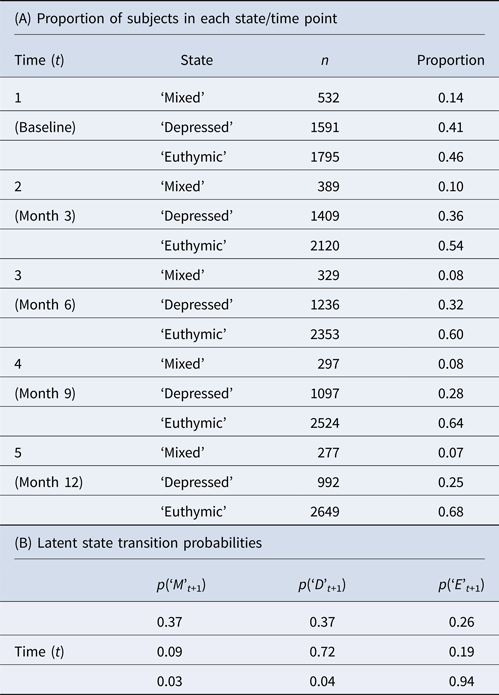
The probability of transitioning between, or remaining in, latent states across time, along with the estimated proportion of participants classified in each state at each time point, are presented in Table 3. Membership in the ‘euthymic’ and ‘depressed’ states was prevalent and relatively stable over time; 94% of participants classified as euthymic at any given time point were classified as ‘euthymic’ at the next time point, and 72% of participants classified as ‘depressed’ were classified as ‘depressed’ at the next time point. Averaging across time, approximately 58% of the sample was classified as ‘euthymic’ and 32% was classified as ‘depressed.’ Conversely, membership in the ‘mixed’ state was limited (9% of the sample, on averaging across time) and highly variable; approximately one-third of participants classified as ‘mixed’ at any given time point were classified as ‘mixed’ at the next time point, with the remaining two-thirds split roughly equally between ‘depressed’ and ‘euthymic’ states.
Table 3. Proportion of subjects classified in each state at each time point and latent state transition probabilities

Proportion, proportion of the sample classified in a given latent state at a given point in time; P, probability of being classified in a particular latent state at the subsequent time point; M, Mixed; D, Depressed; E, Euthymic.Note. Latent state transition probabilities were fixed across contiguous pairs of time points (e.g., transition probabilities for t = 1 to t = 2 were the same as probabilities for t =2 to t = 3 and so on).
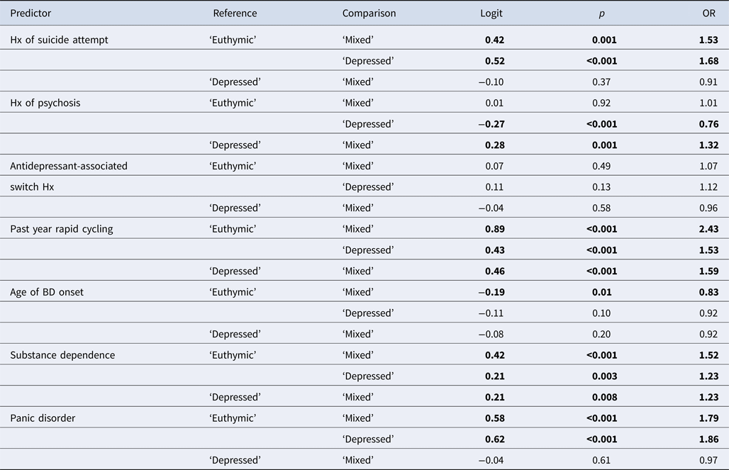
Given that the ‘euthymic’ and ‘depressed’ states were well-defined, stable, and conceptually clear, we primarily selected baseline covariates for the final HMM model that have been shown in past research to be associated with mixed episodes in order to clarify the conceptual nature of the obtained ‘mixed’ state. These variables included: history of suicide attempt, history of psychosis, history of antidepressant-associated switch, past year rapid cycling, age of BD onset, lifetime substance dependence, and panic disorder (Perlis et al., Reference Perlis, Miyahara, Marangell, Wisniewski, Ostacher, Delbello, Bowden, Sachs and Nierenberg2004, Reference Perlis, Ostacher, Goldberg, Miklowitz, Friedman, Calabrese, Thase and Sachs2010; Schneck et al., Reference Schneck, Miklowitz, Miyahara, Araga, Wisniewski, Gyulai, Allen, Thase and Sachs2008; Goldberg et al., Reference Goldberg, Perlis, Bowden, Thase, Miklowitz, Marangell, Calabrese, Nierenberg and Sachs2009; Ostacher et al., Reference Ostacher, Perlis, Nierenberg, Calabrese, Stange, Salloum, Weiss and Sachs2010; Niitsu et al., Reference Niitsu, Fabbri and Serretti2015); a wider range of covariates was not considered in order to maintain a reasonable experimentwise alpha level. Because mood symptoms were best represented by three latent states, associations between covariates and latent states were estimated in a multinomial logistic regression framework. As depicted in Fig. 1, reported covariate effects are independent of potentially correlated first order autoregressive effects. To obtain the full range of desired between-state comparisons, the conditional model was estimated twice, once with ‘euthymic’ as the reference state and again with ‘depressed’ as the reference state. Regression coefficients and odds ratios are presented in Table 4. As can be seen in Table 4, history of suicide attempt, past year rapid cycling, panic disorder, lifetime substance use disorder, and younger age of onset were all significantly associated with transitioning to or remaining in the ‘mixed’ v. ‘euthymic’ state. Most of these covariates (i.e. history of suicide attempt, past year rapid cycling, panic disorder, and lifetime substance use disorder) were also significantly associated with transitioning to or remaining in the ‘depressed’ v. ‘euthymic’ state. In contrast, history of psychosis was significantly associated with transitioning to or remaining in the ‘euthymic’ v. ‘depressed’ state. Importantly, however, three covariates (past year rapid cycling, lifetime substance use disorder, and history of psychosis) incrementally predicted transitioning to or remaining in the ‘mixed’ v. ‘depressed’ state. In sum, whereas history of suicide attempt, panic disorder, and age of BD onset similarly predicted transitioning to or remaining in the ‘mixed’ or ‘depressed’ state, past year rapid cycling, substance use disorder, and history of psychosis predicted transitioning to or remaining in the ‘mixed’ state significantly more strongly than they predicted transitioning to or remaining in the ‘depressed’ state.
Table 4. Associations between baseline covariates and probabilities of remaining in or transitioning between latent states from one time point to the next

Hx, history; BD, bipolar disorder.
Note: Covariate effects reported are above and beyond the effect of latent class membership at a given time point on remaining in or transitioning to latent states at the subsequent time point (i.e. first order autoregressive effects). Associations between covariates and latent states were estimated in a multinomial logistic regression framework: ‘reference’ = reference group and ‘comparison’ = comparison group for a given logit. Significant effects (i.e. p < 0.05) are bolded.
Discussion
The current study used advanced longitudinal statistical modeling to simultaneously identify three latent mood states (‘euthymic,’ ‘depressed,’ and ‘mixed’) and characterize transitions among these mood states over time in 3229–3918 outpatients (depending on analysis) with BD. Unlike the euthymic and depressed latent mood states, the mixed state was relatively unstable across time (i.e. assignment to the mixed state at a given time point equally predicted assignment to any of the three identified mood states at the subsequent time point) and was uniquely associated with rapid cycling, substance use, and psychosis. Descriptively, individuals assigned to the latent mixed state at baseline were relatively more likely to be diagnosed with a current mixed, manic, or hypomanic episode, and reported spending more time experiencing irritable and elevated mood in the preceding year relative to individuals assigned to euthymic or depressed states. Although they were also relatively less likely to be diagnosed with bipolar II (v. I) disorder, nearly 25% of individuals assigned to the mixed state at baseline were diagnosed with bipolar II disorder nonetheless, supporting the changes in how mixed symptoms are characterized in DSM-V relative to DSM-IV (which precluded the diagnosis of mixed episodes in bipolar II disorder by definition).
These findings are concordant with a recent study that identified ‘stable’ (i.e. primarily euthymic), ‘depressive’ [i.e. more prominent depression (i.e. 23% of the time) than the ‘stable’ class (i.e. 8% of the time)] and ‘rapid-cycling’ [i.e. somewhat less prominent depression (i.e. 17% v. 23% of the time) but more prominent mania (i.e. 13% v. 7% of the time) relative to the ‘depressive’ class] classes of mostly female outpatients with bipolar I disorder (Cochran et al., Reference Cochran, Mcinnis and Forger2016); Cochran's study used a similar statistical methodology as in the current study, but with a relatively smaller sample (i.e. n = 209) combined with a large number of retrospectively obtained data points [i.e. taken from a single administration of the Longitudinal Interval Follow-up Evaluation (LIFE) (Denicoff et al., Reference Denicoff, Leverich, Nolen, Rush, Mcelroy, Keck, Suppes, Altshuler, Kupka, Frye, Hatef, Brotman and Post2000)]. Their primary finding was that ‘rapid-cycling’ participants experienced a greater degree of functional impairment and disability relative to ‘stable’ and ‘depressive’ participants. With continued empirical support, this emerging literature could provide clinicians and researchers with important predictive information about their patients and participants.
Based on both the current findings and the extent of literature, individuals with BD who present to the research and/or treatment clinic with elevated levels of both depression and mania are likely experiencing a state that is transient yet clinically dangerous (Pallaskorpi et al., Reference Pallaskorpi, Suominen, Ketokivi, Valtonen, Arvilommi, Mantere, Leppamaki and Isometsa2017). They may be at high risk for substance use and further mixed and depressive mood episodes, and they are more likely to have a history of psychosis. In short, they are different from individuals presenting with depression or euthymia in important ways that indicate elevated severity and risk for deleterious outcomes. Clearly, in the case of patients presenting to the clinic, these predictions could provide important guidance to clinicians regarding treatment and likely course. Results from the current study could also be used to define potential ranges and/or cut-offs on the most commonly utilized clinician-administered bipolar mood assessments (i.e. YMRS and MADRS) that could be used to diagnose euthymic, depressive, and mixed mood states in outpatients with BD. These cut-offs would represent a relatively objective and opinion-agnostic method of mood state (‘episode’) definition derived from longitudinal mood data on a very large sample of bipolar outpatients, in contrast to the current method that consists of using an assessment with more limited psychometric properties (i.e. the Structured Clinical Interview for DSM-IV Disorders) to diagnose mood states that have been defined by expert opinion (e.g. at least five of nine clinically significant depressive symptoms, necessarily including depressed mood and/or anhedonia, that have been present most of the time for at least 2 weeks – ‘Major Depressive Episode’ ala DSM-5). Using these empirically defined mood states as building blocks, future studies could examine more frequently collected (i.e. weekly) YMRS and MADRS data to identify characteristic longitudinal patterns of mood dysfunction which could be used to classify patients into meaningful subtypes that are defined by mood state course. We have avoided doing so in the current study because reliable and valid assessments of bipolar mood symptoms were obtained only quarterly in the STEP-BD study, precluding a more temporally granular examination of transitions between mood states. Cochran and colleagues’ investigation may provide a first step toward such granular examination of mood state transitions suggesting individuals with bipolar I disorder can be divided into ‘stable’ (i.e. predominantly euthymic), ‘depressive’ (i.e. predominantly euthymic but depressed approximately 20% of the time), and ‘rapid-cycling’ (i.e. predominantly euthymic but with more time spent in mania relative to depressive patients and more transient mood episodes overall) (Cochran et al., Reference Cochran, Mcinnis and Forger2016). However, given the relatively small sample, overrepresentation of females (i.e. potential lack of generalizability), and psychometric weaknesses of the retrospectively assessed symptomatology information, further research may be needed to provide more confidence to their findings. Many suitable data sets for the suggested investigation already exist in the form of completed clinical trials for BD, many (and perhaps most) of which used weekly administrations of the MADRS and YMRS to evaluate treatment outcome.
Although the current study has a number of unique strengths (e.g. large naturalistic sample of individuals with BD, repeated clinician-administered assessment of depressive and manic symptoms using valid and reliable instruments, and sophisticated statistical methodology), it also suffers from notable weaknesses. First, although the current study defined latent mood states and transitions among mood states using longitudinal data, each contiguous pair of assessments was separated by 3 months. Second, a relatively limited subset of clinically relevant variables was examined in relation to the empirically defined mood states in order to reduce experimentwise alpha inflation. Third, to maximize our ability to identify latent mood states with potentially sparse patient assignment at any given time point, we did not evaluate the replicability of the obtained mood states within the STEP-BD data. Nor did we evaluate the construct validity of models containing four to six latent mixtures per time point. However, we provided definitions of these additional mixtures, in terms of YMRS and MADRS scores, in hopes that this information may provide an impetus for further research. Fourth, the current study was limited to outpatient individuals which naturally restricted the incidence of acute manic symptoms in the sample, as can be seen by the low reported base rate of acute manic episodes at baseline (Table 1) (Carragher et al., Reference Carragher, Weinstock and Strong2013). As such, the absence of an obtained latent (hypo)manic state in the current study was likely largely due to methodological limitations. In addition to poor representation of individuals experiencing acute mania in the STEP-BD study, the psychometric measure used to measure (hypo)manic symptoms in the study (i.e. YMRS) has been shown to suffer from notable psychometric limitations, including poor coverage of average or below-average outpatient levels of manic symptoms (Prisciandaro and Tolliver, Reference Prisciandaro and Tolliver2016). In sum, additional supportive studies will be needed before the symptom thresholds derived from the current study can be used with confidence to define mood states in future research or clinical decision making.
These limitations notwithstanding, the results from the current study represent an important first step in defining, and characterizing the longitudinal course of, empirically derived mood states that can be used to form the foundation of objective, empirical attempts to define meaningful subtypes of affective illness defined by clinical course.
Acknowledgements
STEP-BD Data Use Certification for Public Release Dataset version 4.1 provided 27 April 2011 (Tolliver, Recipient PI). Data used in the preparation of this article were obtained from the limited access datasets distributed from the NIH-supported ‘Systematic Treatment Enhancement Program for Bipolar Disorder’ (STEP BD). This is a multisite, clinical trial studying the current treatments for BD, including medications and psychosocial therapies. This study was supported by NIMH contract no. N01MH80001 to Massachusetts General Hospital and the University of Pittsburgh. The ClinicalTrials.gov identifier is NCT00012558. This manuscript reflects the views of the authors and may not reflect the opinions or views of the STEP BD Study Investigators or the NIH.
Financial support
Dr Prisciandaro was funded by K23 AA020842.
Conflict of interest
None.