


A person who eventually develops a severe psychotic disorder (e.g. schizophrenia) usually shows signs early in life, years before the disorder is formally diagnosed (Keith & Matthews, Reference Keith and Matthews1991; Yung & McGorry, Reference Yung and McGorry1996). Symptoms in the early ‘pre-disorder’ stage—formerly called the ‘prodrome’—allow care providers and researchers to assess the risk of future conversion to a disorder like schizophrenia (Nelson & McGorry, Reference Nelson and McGorry2020; Yung et al., Reference Yung, Phillips, Yuen, Francey, McFarlane, Hallgren and McGorry2003). Indeed, the discovery of the prodrome and even earlier pre-morbid symptoms (Brown, Reference Brown1963; Mahler, Reference Mahler1952) widened the view of psychosis from a disorder of early adulthood to a disorder of the lifespan (Friedman et al., Reference Friedman, Harvey, Coleman, Moriarty, Bowie, Parrella and Davis2001; Powers et al., Reference Powers, Addington, Perkins, Bearden, Cadenhead, Cannon and Walker2020). This perspective, in turn, has led to substantial research on signs and symptoms that might be detected before the transition to psychosis (Miller et al., Reference Miller, McGlashan, Woods, Stein, Driesen, Corcoran and Davidson1999; Woodberry, Shapiro, Bryant, & Seidman, Reference Woodberry, Shapiro, Bryant and Seidman2016). A promising potential of measuring such symptoms is that psychosis risk and transition can be predicted.
Assessing risk – i.e. estimating the probability of an event occurring given some known information – has been an integral part of medicine's role in prognosis (Combe, Donkin, Buchanan, & Mackenzie, Reference Combe, Donkin, Buchanan and Mackenzie1820). The Framingham study (Dawber, Moore, & Mann, Reference Dawber, Moore and Mann1957) and subsequent analyses (Mahmood, Levy, Vasan, & Wang, Reference Mahmood, Levy, Vasan and Wang2014) showed compellingly that statistical models can predict the future better than the average clinician. Some successful contemporary calculators assess risk, for example, of complications from cardiac surgery (Gupta et al., Reference Gupta, Gupta, Sundaram, Kaushik, Fang, Miller and Lynch2011), complications from pancreatectomy (Parikh et al., Reference Parikh, Shiloach, Cohen, Bilimoria, Ko, Hall and Pitt2010), general surgical complications (Bilimoria et al., Reference Bilimoria, Liu, Paruch, Zhou, Kmiecik, Ko and Cohen2013), undiagnosed diabetes (Heikes, Eddy, Arondekar, & Schlessinger, Reference Heikes, Eddy, Arondekar and Schlessinger2008), periodontal disease (Page, Krall, Martin, Mancl, & Garcia, Reference Page, Krall, Martin, Mancl and Garcia2002), bone fracture risk (Leslie & Lix, Reference Leslie and Lix2014), and hundreds more. Notably, risk calculators have more recently included ‘mental’ illnesses like psychosis, the focus of the present study. Cannon et al. (Reference Cannon, Yu, Addington, Bearden, Cadenhead, Cornblatt and Perkins2016) developed a calculator for risk of conversion from clinical high risk (CHR) to frank psychosis within a 2-year window using time-to-event (Cox) regression. They found that psychosis conversion was best predicted by positive psychosis symptoms, declining social function, and poor verbal learning. This calculator was later replicated and extended by Carrión et al. (Reference Carrión, Cornblatt, Burton, Tso, Auther, Adelsheim and Taylor2016), Zhang et al. (Reference Zhang, Li, Tang, Niznikiewicz, Shenton, Keshavan and Wang2018) and Osborne and Mittal (Reference Osborne and Mittal2019). Fusar-Poli et al. (Reference Fusar-Poli, Rutigliano, Stahl, Davies, Bonoldi, Reilly and McGuire2017, Reference Fusar-Poli, Oliver, Spada, Patel, Stewart, Dobson and McGuire2019) developed a calculator to forecast the transdiagnostic risk of developing psychosis in secondary care, where predictors (demographics and any index diagnosis of non-psychotic mental disorder) were selected based on a priori knowledge [see Riecher-Rossler and Studerus (Reference Riecher-Rössler and Studerus2017), Radua et al. (Reference Radua, Ramella-Cravaro, Ioannidis, Reichenberg, Phiphopthatsanee, Amir and Fusar-Poli2018), Adibi, Sadatsafavi, and Ioannidis, (Reference Adibi, Sadatsafavi and Ioannidis2020), and Sanfelici, Dwyer, Antonucci, and Koutsouleris (Reference Sanfelici, Dwyer, Antonucci and Koutsouleris2020) for reviews].
Importantly, currently available psychosis risk calculators were developed in individuals who were seeking clinical care because of psychosis spectrum (PS) symptoms, and thus apply to youth who are already experiencing some distress and/or impairment. A complementary approach to risk identification is through general population or community samples, which aims the ascertainment lens at a broader range of individuals experiencing PS symptoms (Taylor, Calkins, & Gur, Reference Taylor, Calkins and Gur2020; Wigman et al., Reference Wigman, van Winkel, Raaijmakers, Ormel, Verhulst, Reijneveld and Vollebergh2011). This approach may allow earlier identification of at-risk youth and commensurate enhanced opportunities to evaluate varying developmental trajectories and targeted early interventions. Among the few prospective studies in this area, several consistent findings have emerged indicating that persistence and worsening of PS symptoms are associated with particular symptoms, neurocognitive deficits, and neuroimaging parameters and other biomarkers (Calkins et al., Reference Calkins, Moore, Satterthwaite, Wolf, Turetsky, Roalf and Gur2017; Davies, Sullivan, & Zammit, Reference Davies, Sullivan and Zammit2018; Kalman, Bresnahan, Schulze, & Susser, Reference Kalman, Bresnahan, Schulze and Susser2019; Taylor et al., Reference Taylor, Calkins and Gur2020). The development and application of a community applied psychosis risk calculator could greatly facilitate the aims of such endeavors, potentially accelerating discoveries and treatment innovations earlier in the pathway to care than is currently feasible.
Given the moderate success of prior CHR calculators, but the different ascertainment strategies of CHR and community-based cohorts, which can have a substantial role in enriching the risk to psychosis (Fusar-Poli et al., Reference Fusar-Poli, Schultze-Lutter, Cappucciati, Rutigliano, Bonoldi, Stahl and Woods2016), a critical question is whether prior calculators are applicable to community samples. The present study, therefore, had two goals. First, we aimed to evaluate the construct validity (Cronbach & Meehl, Reference Cronbach and Meehl1955, pp. 282–283) of the Cannon et al. (Reference Cannon, Yu, Addington, Bearden, Cadenhead, Cornblatt and Perkins2016) psychosis risk calculator of the North American Prodrome Longitudinal Study (NAPLS) in the Philadelphia Neurodevelopmental Cohort (PNC), using variables as similar as possible to those used in the original study. Second, we aimed to develop and internally validate a new calculator designed to predict the risk of PS status in a community cohort of young people aged 8–21. That is, rather than focus on the transition to threshold psychosis, which may be the optimal focus for clinical applications, we focus on the risk of occurrence of PS symptoms in youth, which has practical scientific purposes such as evaluating neurodevelopmental biobehavioral trajectories in a youth sample enriched with potential for transition to psychosis.
Methods
Participants
Participants (n = 632) were recruited for follow-up based on Time 1 PS screening of the PNC (Calkins et al., Reference Calkins, Moore, Merikangas, Burstein, Satterthwaite, Bilker and Gur2014, Reference Calkins, Merikangas, Moore, Burstein, Behr, Satterthwaite and Gur2015; Moore et al., Reference Moore, Martin, Gur, Jackson, Scott, Calkins and Gur2016). PNC participants at Time 1 included ~10 000 genotyped youth aged 8–21 years at enrollment (2009–2011), recruited from pediatric, non-psychiatric services of the Children's Hospital of Philadelphia (CHOP) health care network. The youth were in stable health, proficient in English, and physically and cognitively capable of participating in a clinical assessment interview and computerized neurocognitive testing. Participants provided informed consent/assent and permission to re-contact after receiving a complete description of the study and the Institutional Review Boards at Penn and CHOP approved the protocol. As detailed previously (Calkins et al., Reference Calkins, Moore, Satterthwaite, Wolf, Turetsky, Roalf and Gur2017), participants who screened either positive (n = 265) or negative (n = 367) for PS symptoms at Time 1 were identified for follow-up assessment if they were physically healthy at Time 1 (no moderate or severe physical conditions requiring multiple procedures and monitoring), had completed the neuroimaging protocol > = 18 months previously, and had good quality neuroimaging data. We emphasized for follow-up individuals from the PNC random subsample (N = 1601) who had also received multimodal neuroimaging at T1 (as detailed in Satterthwaite et al., Reference Satterthwaite, Elliott, Ruparel, Loughead, Prabhakaran, Calkins and Gur2014). Follow-up intervals ranged from 2 to 80 months (mean months = 42.9, s.d. = 16.5). Table 1 provides the Time 1 demographic characteristics of the sample, as well as rates of common mental disorders.
Table 1. Time 1 sample demographic and clinical information for full sample (N = 632)

Note. Values are proportions unless otherwise specified; yrs = years; s.d. = standard deviation.
Measures
Clinical assessment
Details of Time 1 (Calkins et al., Reference Calkins, Moore, Merikangas, Burstein, Satterthwaite, Bilker and Gur2014, Reference Calkins, Merikangas, Moore, Burstein, Behr, Satterthwaite and Gur2015; Moore et al., Reference Moore, Martin, Gur, Jackson, Scott, Calkins and Gur2016) and follow-up (Calkins et al., Reference Calkins, Moore, Satterthwaite, Wolf, Turetsky, Roalf and Gur2017) assessments have been reported. Briefly, at Time 1, probands (age 11–21) and collaterals (parent or legal guardian for probands aged 8–17) were administered a computerized structured interview (GOASSESS). This instrument assessed psychiatric and psychological treatment history, and lifetime occurrence of major domains of psychopathology – including mood, anxiety, behavioral and eating disorders – and suicidal thinking and behavior (Calkins et al., Reference Calkins, Moore, Merikangas, Burstein, Satterthwaite, Bilker and Gur2014, Reference Calkins, Merikangas, Moore, Burstein, Behr, Satterthwaite and Gur2015). Three screening tools to assess PS symptoms were embedded within the psychopathology screen. Positive sub-psychotic symptoms in the past year were assessed with the 12-item assessor administered PRIME Screen-Revised (PS-R) (Kobayashi et al., Reference Kobayashi, Nemoto, Koshikawa, Osono, Yamazawa, Murakami and Mizuno2008; Miller et al., Reference Miller, Cicchetti and Markovich2004). Items were self-rated on a 7-point scale ranging from 0 (‘definitely disagree’) to 6 (‘definitely agree’). Positive psychotic symptoms (lifetime hallucinations and delusions) were assessed using the Kiddie-Schedule for Affective Disorders and Schizophrenia (K-SADS) (Kaufman et al., Reference Kaufman, Birmaher, Brent, Rao, Flynn, Moreci and Ryan1997) psychosis screen questions, supplemented with structured questions to reduce false positives. Negative/disorganized symptoms were assessed using six embedded assessor rated items from the Scale of Prodromal Symptoms (SOPS) (McGlashan et al., Reference McGlashan, Miller and Woods2003).
History of exposure to traumatic stressors was tabulated from the post-traumatic stress disorder section of the GOASSESS, in which participants were asked about lifetime history of experiencing eight categories of events (i.e. natural disasters, witnessed violence, attacked physically, sexually assaulted/abused, threatened with a weapon, experienced a serious accident, witnessed serious physical injury/death, observed dead body).
Global function was rated using the Children's Global Assessment Scale (Shaffer et al., Reference Shaffer, Gould, Brasic, Ambrosini, Fisher, Bird and Aluwahlia1983).
An abbreviated version of the Family Interview for Genetic Studies (FIGS) (Maxwell, Reference Maxwell1996), administered to collaterals (of probands <age 18) and adult probands, screened for presence or absence of a first-degree family history of major domains of psychopathology, with a more detailed assessment of possible psychotic disorders following affirmative responses to psychosis-related screening items. To avoid the influence of proband status on judgments about psychosis family history, the presence/absence was coded based on FIGS data contained in a blinded file, without reference to proband status at either Time 1 or follow-up (Calkins et al., Reference Calkins, Moore, Satterthwaite, Wolf, Turetsky, Roalf and Gur2017; Taylor et al., Reference Taylor, Asabere, Calkins, Moore, Tang, Xavier and Gur2020).
At follow-up, psychopathology was assessed using a custom protocol (Calkins et al., Reference Calkins, Moore, Satterthwaite, Wolf, Turetsky, Roalf and Gur2017) consisting of modules of the K-SADS and the Structured Interview for Prodromal Syndromes (SIPS, version 4.0) (McGlashan et al., Reference McGlashan, Miller and Woods2003) administered to probands (age 11 and up) and collaterals (of probands age 8–17). Following each evaluation, assessors integrated information from probands, collaterals, and available medical records to provide combined ratings across symptom domains. Integrated clinical information was then summarized in a narrative case history and presented at a case conference attended by at least two doctoral-level clinicians with expertise in psychosis and/or child psychopathology. Strict blinding was maintained such that recruiters, assessors and clinicians determining consensus ratings and diagnoses were naive to Time 1 PS screening status of all participants. To avoid biasing case assignment or symptom ratings, family history of psychopathology was not disclosed during the case conference. Each SOPS clinical rating ⩾3 based on the SIPS interview underwent consensus review, and clinical risk status and best estimate final diagnoses for Axis I disorders were determined. Individuals were classified as meeting PS criteria if they had either (a) a DSM-IV psychotic disorder or mood disorder with psychotic features, or (b) at least one SOPS positive symptom currently (past 6 months) rated 3–5 or at least two negative and/or disorganized symptoms rated 3–6. See Calkins et al. (Reference Calkins, Moore, Satterthwaite, Wolf, Turetsky, Roalf and Gur2017) for detailed training and assessment procedures.
Neurocognitive assessment
Time 1 neurocognition was assessed using the Penn Computerized Neurocognitive Battery (Penn CNB) (Gur et al., Reference Gur, Ragland, Moberg, Turner, Bilker, Kohler and Gur2001, Reference Gur, Richard, Hughett, Calkins, Macy, Bilker and Gur2010; Moore, Reise, Gur, Hakonarson, & Gur, Reference Moore, Reise, Gur, Hakonarson and Gur2015), which comprises 14 tests grouped into five domains of neurobehavioral function. A full description of the Penn CNB, including a description of each individual test, is available in the Supplement.
Environmental exposures
Time 1 environment was assessed using a combination of, (1) self-reported traumatic experiences (as described above), and (2) neighborhood-level characteristics obtained by geocoding participants addresses to census and crime data in the Philadelphia area. Neighborhood characteristics were measured at the block-group level and included median family income, percent of residents who are married, percent of real estate that is vacant, and several others; see Moore et al. (Reference Moore, Martin, Gur, Jackson, Scott, Calkins and Gur2016) for further details.
Statistical analyses
Quasi-Replication of Cannon et al. (Reference Cannon, Yu, Addington, Bearden, Cadenhead, Cornblatt and Perkins2016)
The first goal of the present study was to replicate in the PNC the psychosis risk calculator results presented in Cannon et al. (Reference Cannon, Yu, Addington, Bearden, Cadenhead, Cornblatt and Perkins2016), but note that a true replication (using the same variables and coefficients as in the published model) was not possible here. Our approach – testing most of the same variables as in the NAPLS study after re-estimating the coefficients – is best characterized as a ‘quasi-replication’ in the terminology of Coiera, Ammenwerth, Georgiou, and Magrabi (Reference Coiera, Ammenwerth, Georgiou and Magrabi2018).
NAPLS identified the following variables as useful predictors of conversion from a CHR state to frank psychosis within 2 years: age, sum of Structured Interview for Psychosis-risk Syndromes (SIPS) items P1 (Unusual Thought Content) and P2 (Suspiciousness), the Brief Assessment of Cognition in Schizophrenia (BACS) symbol coding raw score, Hopkins Verbal Learning Test (HVLT), stressful life events, family history of psychosis, Global Scale of Functioning-Social (GFS-S) (decline in functioning), and traumatic events (>1). In addition to being useful predictors, the variables identified in the NAPLS study are supported by previous studies and can be obtained in general clinical settings. To replicate the findings of Cannon et al. (Reference Cannon, Yu, Addington, Bearden, Cadenhead, Cornblatt and Perkins2016), we first selected variables in the PNC that most closely match the variables listed above. Online Supplementary Table S1 shows the NAPLS-2 variables used, along with their PNC equivalents. We had perfect or near-perfect matches for Age, Family History, and Traumatic Events, and only partial matches for SIPS P1 & P2, BACS symbol coding, HVLT, and GFS-S. No equivalent was found for stressful life events, though this is partly captured in the traumatic events count. In addition, the PNC sample in this specific replication analysis was limited to those who started the study (Time 1) with subthreshold PS symptoms (same N = 265 PS positive detailed in the Participants sub-section), which is different from the data set (full N = 632) used for the construction of the new calculator (see below). This was done because the NAPLS calculator was meant to predict the transition from high-risk to frank psychosis and did not include low-risk people. Thus, the NAPLS-2 calculator was designed to detect a frank psychosis outcome in a sample of people with CHR, whereas the PNC-based calculator was designed to detect CHR/PS in a sample of non-help-seeking community participants. The outcome of interest was (binary) transition to threshold psychosis (N = 26 out of the 265) within 2 years of the first visit. As in Cannon et al. (Reference Cannon, Yu, Addington, Bearden, Cadenhead, Cornblatt and Perkins2016), a Cox proportional hazards model (survival analysis) was used. The main metric used for assessment of prediction accuracy was area under the receiver operating characteristic (ROC) curve (Hanley & McNeil, Reference Hanley and McNeil1982).
PNC-based risk calculator
Next, we wished to build a new psychosis risk calculator within parameters more appropriate to our whole longitudinal sample (N = 632, which includes the N = 265 CHR persons used above, plus N = 367 others, most typically developing). Rather than predicting transition from CHR to threshold psychosis, we aimed to predict the milder PS status. For these purposes someone who does the transition to frank psychosis (not the milder ‘psychosis spectrum’) would be included as a ‘case’ here – i.e. we wished to predict transition to PS or frank psychosis.
To construct the PNC-based risk calculator, we combined three feature-selection methods with three prediction methods, completely crossed (for nine total) in a single cross-validated pipeline. Details are given below, but the core procedure involved splitting the data into testing and training sets, selecting variables and building the model in the training set, and then testing it in the testing set. The cross-validated framework was 10-fold, such that all participants received a predicted value based on variables selected (and model built) in 90% of the sample not including him/her. The 10-fold cross-validation was repeated 1000 times.
Selection of variables for the model
We used three different feature-selection algorithms to ensure multiple variable characteristics were considered in selecting them – e.g. in addition to main effects (Lasso), does the variable have a nonlinear relationship with the outcome (random forest), does the variable interact with other variables (moderation) in determining the outcome (Relieff and STIR)? For each (90% // 10%) split of the sample (each of the 10-folds), the algorithms below were run, giving three different sets of ‘optimal’ features for each split (all saved for subsequent analyses). The integer number of features selected was also saved. Brief descriptions of the algorithms follow, and additional detail is available in the Supplement.
1. Lasso regression. Lasso regression is a type of regularized regression that assesses a ‘penalty’ (forced downward bias of coefficients) for both the number of predictors used in the model and the collinearity among them (Tibshirani, Reference Tibshirani1996). Usually, the penalty causes most coefficients to become exactly zero, retaining a confined set of non-redundant predictors for prediction (i.e. features with non-zero coefficients are ‘good’).
2. Random forest importance. The random forest algorithm (Liaw & Wiener, Reference Liaw and Wiener2002) leaves the realm of conventional linear modeling and incorporates decision trees. The first step of these decision trees is to determine which single variable best predicts PS in the training sample. Once that is determined, the algorithm splits the sample into those above v. below the mean on the ‘important’ variable. In these split sub-samples, the algorithm then looks for the most important variable. Those sub-samples are then further split based on their ‘most important’ variables, etc.
3. Relieff and Statistical Inference Relief (STIR). Relieff is an algorithm designed specifically for feature selection and known for being especially sensitive to interactions among features (Le, Urbanowicz, Moore, & McKinney, Reference Le, Urbanowicz, Moore and McKinney2019). Given n cases and p variables, Relieff first chooses a random case. In p-dimensional Euclidean space, the algorithm finds the nearest neighbor that is the same as the random case on the categorical dependent variable (DV) (a ‘hit’) and the nearest neighbor that is different from the random case on the DV (a ‘miss’). For any given variable, if the value of that variable for the randomly drawn case is closer to the ‘hit’ case than to the ‘miss’ case, the variable importance goes up; otherwise, it goes down. STIR adds to the Relieff procedure by calculating p values for the predictors (not used in the traditional Relieff algorithm). This allowed us to more confidently make decisions about inclusion of variables without accepting an arbitrary cutoff.
Comparing cross-validated prediction models
With the most important variables selected, the next step in the pipeline was to estimate a model using one of the three prediction methods; therefore, a total of nine models were estimated in each fold, one for each combination of feature-selection and prediction algorithm. Use of multiple algorithms allowed us to answer, generally, which prediction pipeline is likely to perform best in a ‘final’ model. The prediction algorithms were as follows:
1. Ridge regression. Like lasso regression, ridge regression is a form of regularized regression that assesses penalties on the coefficients and is most often used for cross-validation. A major difference is that ridge regression does not shrink coefficients to zero (as does lasso), which was desirable here because the features had already been selected. It is well-established that ridge regression outperforms conventional linear regression in out-of-sample (i.e. cross-validated) prediction (McNeish, Reference McNeish2015).
2. Random forest. The random forest algorithm is described in the above section. Here the algorithm was used for prediction, whereas it had previously been used only for variable selection.
3. Support vector machines (SVMs). SVMs classify cases by finding a hyperplane that separates them (on all variables) with a maximum distance between the hyperplane and the cases (positive or negative). To illustrate an SVM consider the 2-variable case (two continuous predictor variables, X 1 and X 2) predicting a variable with two possible states (say, ‘infected’ or ‘not infected’). Graphing X 1 and X 2 against each other would yield a scatterplot where each point on the scatterplot was either infected or not infected. It would be possible to draw a line through the cloud of points (scatterplot) that maximally separated the infected from the not infected. This line would be the ‘hyperplane’ separating the points; if we added a third variable (X 3), the line would become a plane, and if we added >1 variable (X 4, X 5, etc.), the plane would become a hyperplane.
Final proposed risk calculator model
The results from the above analyses revealed which combination of feature-selection and prediction algorithms would likely be best in practice (i.e. predict most accurately if used as a risk calculator). A problem with the optimal result (see below) is that it required far too many variables for a risk calculator meant to be used by the public. We, therefore. estimated 10-fold cross-validated prediction accuracy using the top 2 variables from the final suggested model, top 3 variables, top 4, etc., up to the top 10 variables allowed. As expected, at first the cross-validated area under the curve (AUC) increased as variables were added, but it eventually started to decrease with additional variables. The maximum/optimal number of variables was taken as the final model. Once this number was established (3 variables? 8 variables?), the full sample was used to maximize estimation accuracy of the coefficients. Cross-validated prediction accuracy of the model therefore cannot be obtained until it is used in another, external sample.
R scripts used for all analyses above can be found at https://www.mooremetrics.com/psy-risk-supplemental-files/.
Results
Quasi-replication of NAPLS risk calculator
Online Supplementary Table S2 shows the results of the CoxPH model run using the sample of Time 1 PS participants (N = 265 who were on the PS at Time 1, not the full N = 632 who included typically developing youth). The strongest predictor of conversion to frank psychosis in the NAPLS calculator is Age (32% increased odds per age year), followed by PRIME total score (PS-R Total) (4% increased odds per point). Figure 1 shows the ROC curve (black) corresponding to the model in online Supplementary Table S2. Within-sample prediction achieves an AUC of 0.71. To put these results into context, including how well we would expect them to cross-validate out-of-sample, we implemented two analyses. First, we ran 2-fold cross-validation on the model setup from online Supplementary Table S2—i.e. coefficients were estimated in a random 50% of the sample, and this model was tested (AUC obtained) using the left-out 50%. This was repeated so that each person had an out-of-sample prediction, quality of prediction was assessed using conventional metrics (AUCs, etc.), and this was repeated 10 000 times to get a distribution of cross-validated AUCs. The AUCs of the cross-validated models are shown in green in Fig. 1, and as expected, cross-validation reduced the AUC from 0.71 to 0.64, the latter below the conventional cutoff of 0.70.
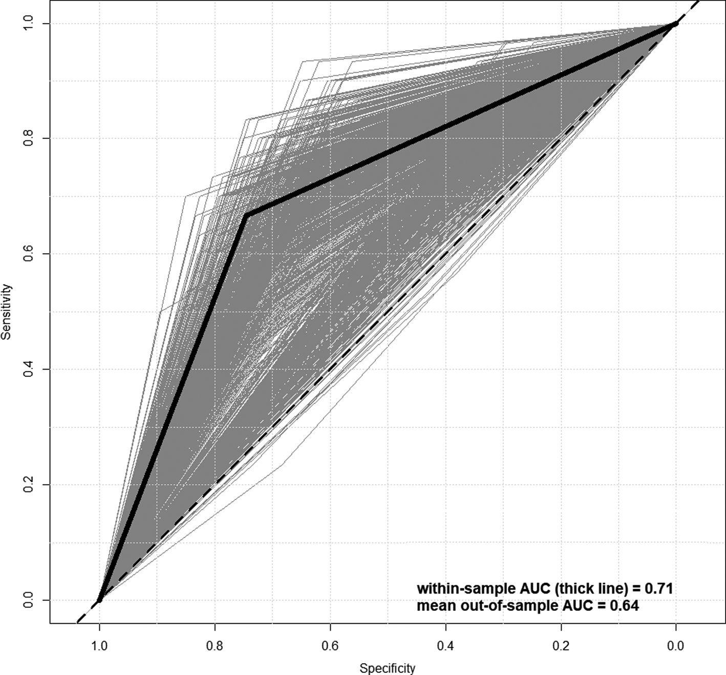
Fig. 1. Receiver operating characteristic curves for within-sample (thick) and out-of-sample (thin, gray) prediction of psychosis conversion.
As a secondary analysis, because we wanted to gauge how ‘impressive’ a within-sample AUC of 0.71 is, we compared the within-sample results (AUC = 0.71; black function in Fig. 1) to ‘random’ within-sample results using permuted labels for Psychosis. That is, the binary indicator for frank Psychosis was randomly reassigned and the model re-estimated, giving a rough indication of what level of within-sample prediction accuracy one could expect purely by chance, given this number of variables distributed in this way with this specific (tiny) proportion of ‘hits’. The above permutation of labels was repeated 10 000 times, and the mean AUC was taken to be the AUC expected by chance. online Supplementary Figure S1 shows the results of the permutation analysis. The pink ‘cloud’ comprises 1000 of the 10 000 ROC curves (limited to 1000 for better visual) estimated for each permutation, and the black function is the same within-sample ROC prediction curve resulting from the model in online Supplementary Table S2. Mean AUC for the permuted labels was 0.60, compared to 0.71 using the correct labels. Of central importance in this test is whether the 0.71 falls within the range of AUCs, we would expect by chance, where the range is defined by the 95% confidence interval. The upper bound of the confidence interval is 0.69, meaning the within-sample AUC value of 0.71 indicates prediction significantly better than chance.
PNC-based risk calculator
Figure 2 shows a comparison of the nine pipelines tested here, by AUC. Quality of prediction algorithms was clear, with ridge being the best (three leftmost bars in Fig. 2), followed by random forest, followed by SVMs. Quality of selection algorithms was more variable, with each of the three demonstrating best performance, depending on the algorithm: random forest selection is best for ridge, lasso selection is best for random forest, and STIR selection is best for SVMs. The key result is that the best cross-validated AUC was achieved using random forest selection, followed by ridge regression for prediction. We also examined the balance of sensitivity and specificity achieved by the pipelines in Fig. 2, shown in online Supplementary Figure S2. In all but one pipeline (RF – >SVM), sensitivity is prioritized over specificity, and this is especially true for the models using the RF predictor (middle three sets of bars in online Supplementary Figure S2).
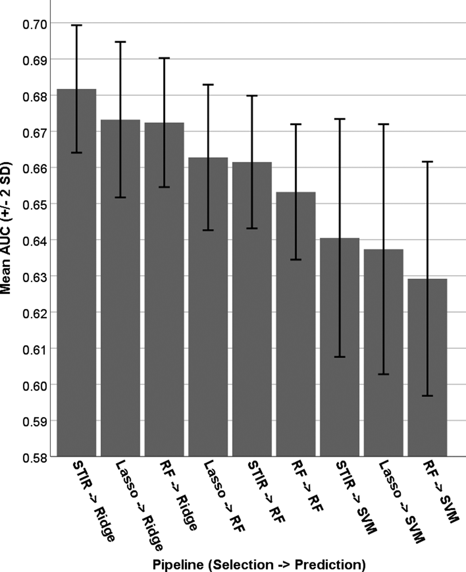
Fig. 2. Area under the ROC curve for nine combinations of feature-selection and prediction algorithms.
Figure 3 shows the frequency of feature-selection across the three algorithms (plus the mean), ordered by decreasing apparent importance overall. The top three most important, on average, were the C-GAS, PS-R item 2 (‘I think that I might be able to predict the future’), and PR-R item 3 (something interrupting or controlling thoughts/actions). Regarding agreement among the three algorithms, the top 10 variables (on average) were in the top 1% of all three algorithms, suggesting substantial agreement, at least at the high importance level. Some notable exceptions include, (1) emotion identification performance was considered extremely important by STIR and random forest but only moderately so by lasso, (2) working memory performance was considered extremely important by STIR and random forest but not important at all by lasso, and (3) currently, taking psychoactive medications was considered extremely important by STIR and lasso but not important at all by random forest. Breaking the top ten variables down into ‘types’, five are clinical, three are cognitive, and two (trauma and percent married in neighborhood) are related to the environment or external experiences. Notably, none of the demographic characteristics was in the top 10; race was considered important (almost top 10), and age and sex were considered only moderately important.

Fig. 3. Frequency of variable selection across random data partitions, by algorithm, in decreasing order of importance.
One problem with the optimal results from Table 2 (STIR – >ridge) is that the average number of variables selected (47.8), on average, was far too many for a risk calculator meant to be used by the public. We, therefore, opted to run a secondary analysis in which we tested the cross-validated prediction performance of increasing numbers of suggested variables. One sensible approach – i.e. to use the importance ranking provided by STIR – was not possible, because too many variables (21) were given the highest possible importance rating by STIR (i.e. selected on all 10 000 runs). To break the 21-way tie, we opted to use the average importance (black line in Fig. 3) in selecting the sequence of variables to add. Note that the final model comprised variables with maximum random forest importance anyway.
Table 2. Final psychosis risk calculator using ridge regression and the top six predictors
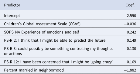
Note. SOPS = Scale of Prodromal Symptoms; PS-R (aka ‘PRIME’) = Prevention through Risk Identification, Management, and Education Screen-Revised; Coef = coefficient; SCR = screen; final result will be in log-odds units, which can be converted to probability by exponentiating (to convert from log-odds to odds) and then using the equation probability = odds/(odds + 1); p values and standard errors are not given because they are not meaningful for this type of model (Goeman, Meijer, & Chaturvedi, Reference Goeman, Meijer and Chaturvedi2018) due to downwardly biased coefficients (typical rules of general linear model, where the equation is the best linear unbiased estimator, do not apply).
Figure 4 shows the cross-validated prediction results using ridge regression and the ‘top x’ variables according to average selection frequency in Fig. 3. With only one variable (C-GAS), the model achieves a CV AUC of almost 0.66. Adding PRIME_2 increases the AUC to almost 0.68, and adding PRIME_3 (for three variables total) brings the CV AUC back down to ~0.66. Adding three more variables (percent married in neighborhood, PRIME_12, and SIPS Perception of Self) brings the CV AUC to its maximum of almost 0.70. The final proposed risk calculation model therefore comprised C-GAS, PRIME_2, PRIME_3, percent married in neighborhood, PRIME_12, and SIPS Perception of Self/Others.

Fig. 4. AUC and balanced accuracy achieved by increasing numbers of variable.
Table 2 shows the coefficients associated with this model. To facilitate use by future researchers, the coefficients in Table 2 are in raw native units (e.g. PS-R responses are on their usual 0–6 scale, C-GAS is out of 100, etc.). Increased risk of psychosis is indicated by low C-GAS; residence in a neighborhood where most people are unmarried; and endorsement of clinical symptoms related to predicting the future, having one's thoughts controlled, concerns about going crazy, or changes in the experience of self/others.
Discussion
We performed a quasi-replication of a previously developed risk calculator for the transition from PS status to threshold psychosis, and then developed a new calculator for prediction of PS-risk status in a community sample.
Replication of the Cannon et al. (Reference Cannon, Yu, Addington, Bearden, Cadenhead, Cornblatt and Perkins2016) calculator was successful insofar as the within-sample prognostic performance of the calculator was comparable across the two studies. Cross-validation of the results revealed predictive performance (AUC = 0.64) below what is traditionally considered adequate (AUC = 0.70), though all results for this replication should be interpreted with caution. First, there was not an exact match of variables used in the original calculator (Cannon et al., Reference Cannon, Yu, Addington, Bearden, Cadenhead, Cornblatt and Perkins2016). For example, we could include here only a broad index of global function (C-GAS), which conflates clinical symptoms and multiple domains of function, whereas NAPLS-2 utilized recent decline in social function assessed with the Global Function Social Scale, which differentiates social function from clinical symptoms and other aspects of functioning (Cornblatt et al., Reference Cornblatt, Carrion, Addington, Seidman, Walker, Cannon and Lencz2012). Second, this was a highly unbalanced sample with <10% cases (converters), meaning one could achieve >90% accuracy simply by predicting that no one will convert. This makes the 74% accuracy of the Cannon model seem unacceptably low, but this phenomenon in highly unbalanced samples will confound most available risk calculators with AUCs <0.80. Also, accuracy is not always the primary objective – e.g. the accuracy-maximizing prediction (mentioned above) that no one will convert would be useless in medicine. Finally, the coefficients in the NAPLS-2 model were re-estimated in this new sample, making this study only a quasi-replication focused on construct validity of the calculator. Despite these limitations, our findings appear to support the generalizability of the risk calculator approach in a broader PS community-based cohort.
Development of a new calculator for risk of future PS status (i.e. risk of being at high risk) revealed numerous important predictors of risk and achieved a cross-validated AUC (0.70 rounded up) that was minimally acceptable by contemporary standards. However, there is some information leakage (Boehmke & Greenwell, Reference Boehmke and Greenwell2020) caused by the fact that the six variables in the final model were chosen based on importance across multiple algorithms across enough random cross-validations that information used for feature-selection ultimately came from the full sample. Therefore, a more conservative estimate of the success of the present risk calculator would be to use the max number in Fig. 2, which is ~0.68. Additionally, a critical feature of the risk calculator presented here is that, unlike prior risk calculators, although we did perform our analyses in a community sample enriched for PS symptoms, the risk calculator was not developed on a clinically help seeking sample, characterized by distress and treatment seeking. Thus, the predictive utility of the calculator must be balanced with the potential stigma and anxiety associated with a risk label (Rüsch et al., Reference Rüsch, Heekeren, Theodoridou, Müller, Corrigan, Mayer and Rössler2015; Yang et al., Reference Yang, Link, Ben-David, Gill, Girgis, Brucato and Corcoran2015). Notably, the model prioritized environment (percent married in neighborhood) over race, suggesting the possibility that, (1) the actual proportion of people married in a neighborhood contains information all the way across the spectrum rather than simply being a proxy for race, and (2) one's environment is at least as important as one's race in determining psychosis risk.
Despite caveats mentioned above, the tool presented here (web link in Supplement) predicts a broader range of the PS continuum than in clinical high-risk samples, which is an advantage since psychosis can originate outside CHR (Lee, Lee, Kim, Choe, & Kwon, Reference Lee, Lee, Kim, Choe and Kwon2018). That is, most risk calculators (including Cannon et al., Reference Cannon, Yu, Addington, Bearden, Cadenhead, Cornblatt and Perkins2016) focus on conversion to frank psychosis, meaning differentiating among people at lower levels of risk (e.g. the difference between someone who responds to PRIME item 1 with a ‘0’ v. someone who responds with a ‘2’) is not a priority. The calculator presented here focuses on assessing risk along the full PS rather than at the moderate-extreme level where one typically sees conversion to frank psychosis. Prediction of PS status in this manner could be useful in recruiting for prospective community cohorts, where predicting that individuals are likely to experience persisting or worsening PS symptoms in the future might be more desirable than predicting likely threshold psychosis in the same time frame. In particular, the risk calculator presented here is applicable for use in a younger cohort of individuals (mean age 15), where conversion to threshold psychosis within only a few years is relatively rarer than in most CHR samples who are, on average, in the late adolescence early adult age range (e.g. Cannon et al., Reference Cannon, Yu, Addington, Bearden, Cadenhead, Cornblatt and Perkins2016; Osborne & Mittal, Reference Osborne and Mittal2019; Zhang et al., Reference Zhang, Li, Tang, Niznikiewicz, Shenton, Keshavan and Wang2018). This risk strategy may be useful in several ways. First, given that persisting subthreshold psychosis symptoms are associated with increased risk of comorbid psychopathology, including mood, anxiety, substance and suicidal ideation, as well as poor global function (see Taylor et al., Reference Taylor, Calkins and Gur2020 for review), risk prediction can facilitate screening and earlier access to mental health care. In addition to providing referral for relief for current symptoms, screening could lead to improved PS symptom monitoring, resilience-building strategies, and, perhaps, prevention efforts. Second, the approach can facilitate prospective studies aiming to elucidate and characterize biobehavioral and functional features of early developmental trajectories of PS symptoms. Such efforts can potentially facilitate a precision medicine approach by establishing mechanistic links among cellular-molecular aberrations and PS symptoms in the general population.
Supplementary material
The supplementary material for this article can be found at https://doi.org/10.1017/S0033291720005231.
Acknowledgements
This work was supported by the Lifespan Brain Institute (LiBI); NIMH grants MH089983, MH107235, MH081902, MH117014, MH09689, MH103654; and the Dowshen Neuroscience Fund.
Conflict of interest
All authors report no conflicts of interest.
Ethical standards
The authors assert that all procedures contributing to this work comply with the ethical standards of the relevant national and institutional committees on human experimentation and with the Helsinki Declaration of 1975, as revised in 2008.


