Introduction
The contribution of ‘environment’ has been investigated across diverse and multiple domains related to health and cognition (Yen & Syme, Reference Yen and Syme1999; McEwen, Reference McEwen2012; Berkman et al. Reference Berkman, Kawachi and Glymour2014; Krabbendam et al. Reference Krabbendam, Hooker and Aleman2014). However, in the context of large-scale genomic studies the focus has been on obtaining individual-level biomarkers or endophenotypes and environment is considered as a monolithic component that is left for future decomposition (e.g. Gur et al. Reference Gur, Nimgaonkar, Almasy, Calkins, Ragland, Pogue-Geile, Kanes, Blanjero and Gur2007; Greenwood et al. Reference Greenwood, Swerdlow, Gur, Cadenhead, Calkins, Dobie, Freedman, Green, Gur, Lazzeroni, Nuechterlein, Olincy, Radant, Ray, Schork, Seidman, Siever, Silverman, Stone, Sugar, Tsuang, Tsuang, Turetsky, Light and Braff2013), even though the importance of environmental factors has been recognized and demonstrated (e.g. Mezuk et al. Reference Mezuk, Li, Cederin, Concha, Kendler, Sundquist and Sundquist2015; Smoller, Reference Smoller2015). Some limited amount of information on the home environment is typically collected from research participants, such as parental education and household income, and demographic characteristics of their communities such as median age, sex ratios, average education level and ethnicity proportions can be extrapolated based on their home address. It is generally assumed that the environment affects the outcome measures in multiple ways, but there is limited time to collect such information, and the emphasis on measuring complex biomarkers precludes deep environmental phenotyping.
The increased availability of large-scale public databases with detailed information on environmental factors now enables probing of environmental effects on research participants after completion of data collection, provided that information has been collected on their residence. Notably, prospective cohort designs are particularly useful for examining environmental influences on disease risk (Manolio et al. Reference Manolio, Bailey-Wilson and Collins2006). Here we will illustrate a methodology for accomplishing such integration in a large prospective cohort and show how this paradigm can help elucidate some environmental associations with biomarkers. The analytic objective was to not only capture the statistical associations of the census-derived social environment characteristics, but to begin to characterize the complex social dynamics that they represent, using the underlying structure of correlation between those characteristics. The Philadelphia Neurodevelopmental Cohort (PNC) participants present an opportunity to harness the robust social diversity of the Philadelphia area and apply appropriate quantitative methodology to examine the association between social environment and neurocognitive performance.
When confronting large complex datasets, as is common in the efforts to dissect environment, exploratory factor and principal components analysis (PCA) of spatially linked, ‘census-like’ data have been applied. As in the present case, the goal is often to reduce a larger number of available variables to a more manageable number of summary variables. These summary variables are then used in larger substantive analyses involving, for example, hypertension-related mortality rates (James & Kleinbaum, Reference James and Kleinbaum1976), neighborhood change (Temkin & Rohe, Reference Temkin and Rohe1998), quality of life (Lo & Faber, Reference Lo and Faber1997; Li & Weng, Reference Li and Weng2007), child maltreatment (Ernst, Reference Ernst2001), chronic pain (Fuentes et al. Reference Fuentes, Hart-Johnson and Green2007 Footnote 1 Footnote †), economic development (Roberts & McBee, Reference Roberts and McBee1968), multiple sclerosis (Lauer, Reference Lauer1994), body mass (Wang et al. Reference Wang, Kim, Gonzalez, MacLeod and Winkleby2007), and use of mental health services (Tello et al. Reference Tello, Jones, Bonizzato, Mazzi, Amaddeo and Tansella2005).
A second goal of factor analyzing social environment data, especially in the geographic and sociological sciences, is to profile the geo-social characteristics of a particular area. For example, Langlois & Kitchen (Reference Langlois and Kitchen2001) examined the PCA structure of economic and social variables in Montreal, and Ray (Reference Ray1971) conducted a very similar analysis across Canada. Comparable analyses with similar purposes have been carried out in Canberra, Australia (Jones, Reference Jones1965), Manhattan (Carey, Reference Carey1966) and Great Britain (summary in Herbert, Reference Herbert1968). Sometimes, as in the present case, these local analyses are conducted with the specific purpose of calculating a summary score that can be used in subsequent analyses. For example, Barros & Victora (Reference Barros and Victora2005) used PCA to develop a geographic wealth score in Brazil, and Havard et al. (Reference Havard, Deguen, Bodin, Louis, Laurent and Bard2008) used PCA to develop a neighborhood-level index of socioeconomic deprivation in France. However, this methodology is rarely used in genomic studies of neurobehavioral domains, and here we describe the application of such a factor analysis to a study of cognition and brain development in a large population-based cohort of genotyped youths. Such an approach helps interpret individual differences in cognitive performance, illustrating the power of integration with environmental data to elucidate potential causes for variability that can separate genetic from environmental processes.
Method
Participants
The participants and recruiting methods of the PNC have been described in detail (Gur et al. Reference Gur, Richard, Hughett, Calkins, Macy, Bilker, Brensinger and Gur2010; Calkins et al. Reference Calkins, Moore, Merikangas, Burstein, Satterthwaite, Bilker, Ruparel, Chiavacci, Wolf, Mentch, Qiu, Connolly, Sleiman, Hakonarson, Gur and Gur2014, Reference Calkins, Merikangas, Moore, Burstein, Behr, Satterthwaite, Ruparel, Wolf, Roalf, Menth, Qiu, Chiavacci, Connolly, Sleiman, Gur, Hakonarson and Gur2015; Moore et al. Reference Moore, Reise, Gur, Hakonarson and Gur2015). The sample included youths (age 8–21) recruited through an NIMH-funded Grand Opportunity study characterizing clinical and neurobehavioral phenotypes in a genotyped prospectively accrued community cohort. All study participants were previously consented for genomic studies when they presented for pediatric services within the Children's Hospital of Philadelphia (CHOP) healthcare network. At that time they provided a blood sample for genetic studies, authorized access to electronic medical records and gave written informed consent/assent to be re-contacted for future studies. Of the 50 540 genotyped subjects, 18 344 met criteria and were randomly selected, with stratification for age, sex and ethnicity.
The sample included ambulatory youths in stable health, proficient in English, physically and cognitively capable of participating in an interview and performing computerized neurocognitive testing. Youths with disorders that impaired motility or cognition (e.g. significant paresis or palsy, intellectual disability) were excluded. Notably, participants were not recruited from psychiatric clinics and the sample is not enriched for individuals who seek psychiatric help. Also, because CHOP services a large area covering the entire greater Philadelphia region and surrounding counties (including parts of New Jersey and Delaware), the geographical distribution of participants was quite wide. A total of 9498 participants enrolled in the study, the majority between November 2009 and September 2011 and were included in this analysis. Participants provided informed consent/assent after receiving a complete description of the study and the Institutional Review Boards at Penn and CHOP approved the protocol.
Measures
Variables were measured or collected at one of three levels: the individual level (e.g. cognitive test scores, age, medical health ratings), the family level (e.g. number of siblings, mother age at birth, family turbulence score), and the census block group/neighborhoodFootnote 2 level (neighborhood crime rates, percentage of neighborhood residents who are female, etc.)Footnote 3 . Our focus was on the reduction of the plethora of variables in the last category, the neighborhood-level variables. These were collected from the 2010 census-based American Community Survey (ACS) and the 2008 police database on crime rates in the Philadelphia area, which included both violent and non-violent crimesFootnote 4 . Examples of census-based variables included median family income, percent of residents who are married, percent of households that are non-familyFootnote 5 , percent of residents with children, percent of residents who speak English, etc. Examples of crime rate variables include aggravated assaults per capita Footnote 6 , theft from automobiles per capita, etc. Note that because the census and police databases provide absolute counts, most of these variables had to be converted to percentages by dividing by the total block-group population.
Results from the computerized neurocognitive assessments are integrated in the structural analysis example described below as summary variables computed using methods described elsewhere (Gur et al. Reference Gur, Richard, Hughett, Calkins, Macy, Bilker, Brensinger and Gur2010; Calkins et al. Reference Calkins, Moore, Merikangas, Burstein, Satterthwaite, Bilker, Ruparel, Chiavacci, Wolf, Mentch, Qiu, Connolly, Sleiman, Hakonarson, Gur and Gur2014, Reference Calkins, Merikangas, Moore, Burstein, Behr, Satterthwaite, Ruparel, Wolf, Roalf, Menth, Qiu, Chiavacci, Connolly, Sleiman, Gur, Hakonarson and Gur2015; Moore et al. Reference Moore, Reise, Gur, Hakonarson and Gur2015). Specifically,
-
(1) Neurocognitive performance test scores (accuracy and speed) were factor scores generated from a battery of twelve tests designed to probe major neurobehavioral domains. Gur et al. (Reference Gur, Richard, Hughett, Calkins, Macy, Bilker, Brensinger and Gur2010) describe the test battery, and details of the factor analyses are in Moore et al. (Reference Moore, Reise, Gur, Hakonarson and Gur2015).
-
(2) Psychopathology scores (such as ‘externalizing’ and ‘psychosis’) were factor scores generated from item-wise analyses of a comprehensive clinical assessment tool, the GOASSESS. A description of the instrument and its administration is provided by Calkins et al. (Reference Calkins, Moore, Merikangas, Burstein, Satterthwaite, Bilker, Ruparel, Chiavacci, Wolf, Mentch, Qiu, Connolly, Sleiman, Hakonarson, Gur and Gur2014), and a description of the methods used for calculating the factor scores used here are available upon request (Calkins et al. unpublished data).
Finally, some individual-level variables were obtained either from the clinical interview cited above or from basic demographics collected during enrollment. These include age, race, gender, trauma exposure (a total count of traumatic experiences from a list of nine), substance use (a total count of non-pharmaceutical substances used in the last year), parent education (mean years of mother and father, unless only one is available), and whether the participant's parents were separated or divorced.
Exploratory factor analysis (EFA)
The 2010 census-based ACS variables and the neighborhood crime rate variables were analyzed separately via EFA in R (R Core Team, 2014). These were performed using many combinations of extraction method (least squares, maximum likelihood, principal axis) and oblique rotation (oblimin, promax, geomin) to check for inconsistency across method. Inconsistency was minimal, and thus results reported here are for the (default) least squares extraction method with oblimin rotation. The unidimensional, two-, and three-factor solutions of the census and crime variables were examined for interpretability, and the cleanest and most interpretable solution was selected for calculating factor scores by the Thurstone (Reference Thurstone1935) method using the factor.scores() command in the R psych package (Revelle, Reference Revelle2013). The scree plot for the census and crime variables was also examined, and was consistent with our judgment of the most interpretable solution. Extraction beyond three factors for either data set showed signs of over-extraction, such as factors comprising only one indicator. Note that race-related variables such as ‘percent white’ were not included in these analyses (or scores), because we wished to analyze specific associations of neighborhood racial composition independent of the summary variables, i.e. we wished to include a separate race-related variable (‘percent white’) in the structural model demonstration described below. EFAs that included neighborhood racial composition differed very little from the analyses presented here, and are available upon request.
Multilevel structural equation model demonstration
The neighborhood-level factor scores were used in combination with the other individual-level variables described above in a demonstrative structural model. Fig. 1 shows the conceptual path diagram describing the model. Due to intra-class correlation, this type of multilevel data usually requires a special kind of modeling called hierarchical linear modeling. In the structural equation modeling (SEM) framework, it is implemented as multilevel SEM (MSEM). The data used here technically involved three levels (individuals within households within neighborhoods); however, as sibling pairs (especially in the same household) enrolled in the study were relatively rare in the sample (1.3%), household-level variables were treated as individual-level variables in the structural analysis. Additionally, because the crime-related variables were measured 2 years earlier than the census-level variables and were therefore based on the 2000 census block groups, they could not be treated as neighborhood-level variables along with the 2010 census-level variables. That is, although the 2000 and 2010 block groups largely overlapped, there were some exceptions, meaning an individual living in the same place in 2000 and 2010 might be assigned to two different block groups in 2000 and 2010. Crime-related variables were therefore treated as individual-levelFootnote 7 crime-exposure variables (from 2008), while the 2010 census variables were treated as neighborhood-level. The end result was a two-level model with census-based ACS variables at the neighborhood level and all other variables at the individual level.
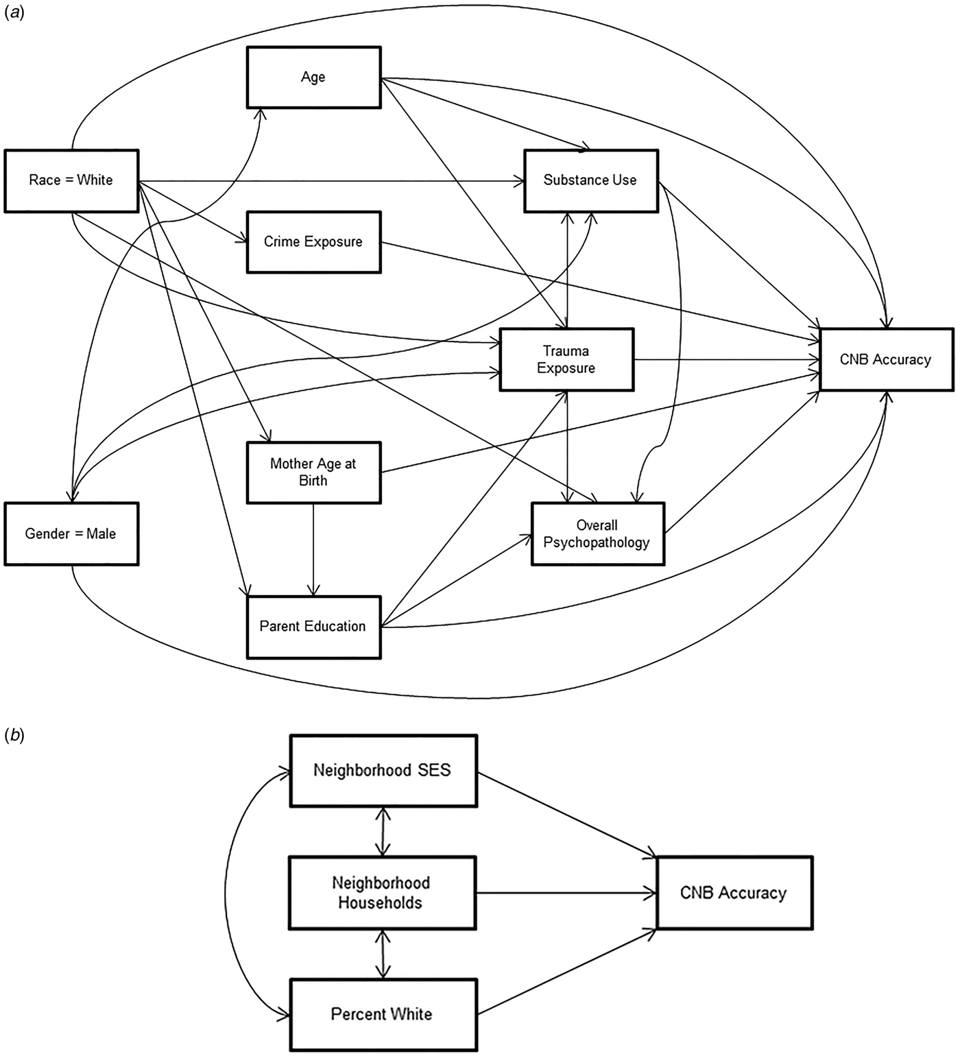
Fig. 1. (a) Structural model (within-level) relating individual-level variables to neurocognitive performance accuracy. (b) Structural model (between-level) relating neighborhood-level variables to neurocognitive performance accuracy.
The variables were related in a MSEM estimated using the robust maximum likelihood estimator in Mplus (Muthén & Muthén, Reference Muthén and Muthén1998–2013). The model revolved around a single dependent variable of interest (neurocognitive test performance accuracy; see Fig. 1), to which all other variables related. To explore mediation, many of the independent variables were related to other independent variables either by direct effect or by correlation. Specific relationships among independent variables were determined by theory and by examining the model modification indices (Sörbom, Reference Sörbom1989).
Results
Exploratory factor analysis
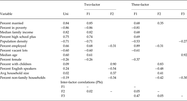
Table 1 shows the unidimensional, two-, and three-factor models for the 13 census-based (block-group-level) variables. The unidimensional model is dominated by socioeconomic status (SES)-related variables, including percent in poverty (−0.86), percent married (0.84), median family income (0.82), and percent with at least a high school education (0.75). Other variables seemingly unrelated to SES have negligible loadings, including average household size (0.02), percent of residents with children (0.09), and percent of households that are non-family (−0.19).
Table 1. Unidimensional, two-, and three-factor solutions of the social environment census variables
Uni, unidimensional; Avg, average; extraction method, least squares; rotation, oblimin.
Loadings with absolute value <0.25 removed in the two- and three-factor models.
The two-factor model in Table 1 retains the SES factor (F1), while the second factor is determined by aspects of household sizes and knowledge of English (regardless of whether it is their first language). As in the unidimensional model, the SES-related factor (F1) is dominated by the percent of residents in poverty, the percent of residents who are married, and the median family income. The household-related factor (F2) is dominated by the percent of residents with children (0.90) and the percent of residents who are English speakers (−0.54). Overall, the two-factor model has a simple structure, with the exception of the cross-loading (−0.31) of percent employed on F2; specifically, those who live in areas with large households and few English speakers are slightly less likely than average to be employed.
The three-factor model in Table 1 is mostly identical to the two-factor model, except that median age has ‘broken away’ from F1 to form its own factor (F3). F3 is completely dominated by median age (loading = 0.92), with only two small negative loadings for population density (−0.27) and percent of households that are non-family (−0.30). That is, older people tend to live in neighborhoods that are less dense and with more family households.
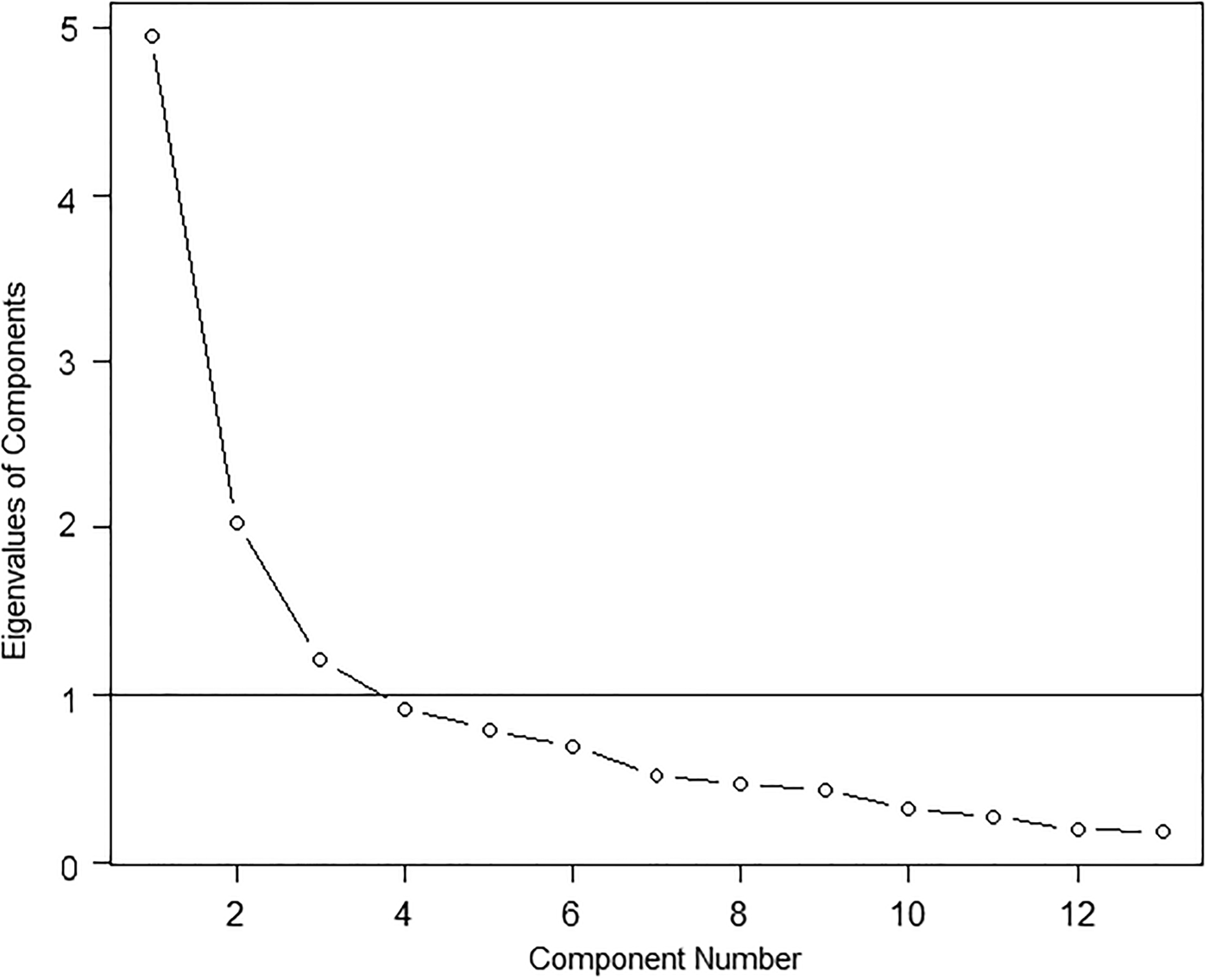
Due to the simple structure and interpretability of the two-factor model (and the lack thereof for the three-factor model), we decided to use the two-factor model for calculating scores. Inspection of the scree plot (Cattell, Reference Cattell1966; see Fig. 2) lends moderate support for this choice of two factors, because that is arguably where the ‘elbow’ of the scree function occurs (see Bentler & Yuan, Reference Bentler and Yuan1998).

Fig. 2. Scree plot of eigenvalues for 13 census-based American Community Survey variables.
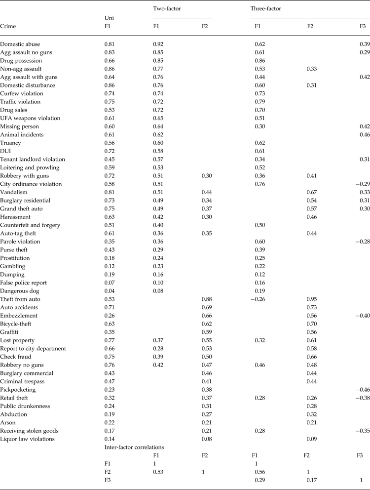
Table 2 shows the unidimensional, two-, and three-factor models of crimes (per 100 persons) committed in Philadelphia neighborhoods in 2008. The unidimensional model is dominated by domestic crimes (disturbance = 0.86, abuse = 0.81) and common assaults (non-aggravated = 0.86; aggravated without guns = 0.83). The weakest indicators are minor crimes (dangerous dog, false police report, gambling, and liquor law violation), all with loadings <0.15. The mean unidimensional loading is 0.52, and the scree plot (Fig. 3) shows a dramatic drop in explained variance when a second factor is extracted (1st:2nd eigenvalue ratio = 5.13). In the two-factor model, F2 largely comprises common, non-violent crimes (theft from auto, auto accidents, embezzlement), whereas F1 retains the violent crimes, as well as other miscellaneous crimes (drug possession, curfew violation, traffic violation). Additionally, there are some notable cross-loadings in the two-factor model; namely, vandalism, grand theft auto, auto-tag theft, lost property, check fraud, and robbery without guns all load on both factors at least 0.35. The three-factor model retains much of the same structure as the two-factor model. One important exception is that the six variables with cross-loadings on F2 in the two-factor model (robbery with guns, vandalism, residential burglary, grand theft auto, harassment, and auto-tag theft) all shift to F2 in the three-factor model. F3 appears to be a contrast factor positively indicated by animal incidents, aggravated assault with guns, and missing persons, and negatively indicated by pickpocketing, embezzlement, and retail theft. Due to the (1) questionable interpretability of the two- and three-factor models, (2) large number of cross-loadings in both models, (3) moderate correlation between F1 and F2 in the two-factor model, and (4) high ratio of 1st:2nd eigenvalues in the unidimensional model, we decided to use the unidimensional model for calculating scores. That is, each individual received a single score for the amount of crime (per capita) in his/her area.
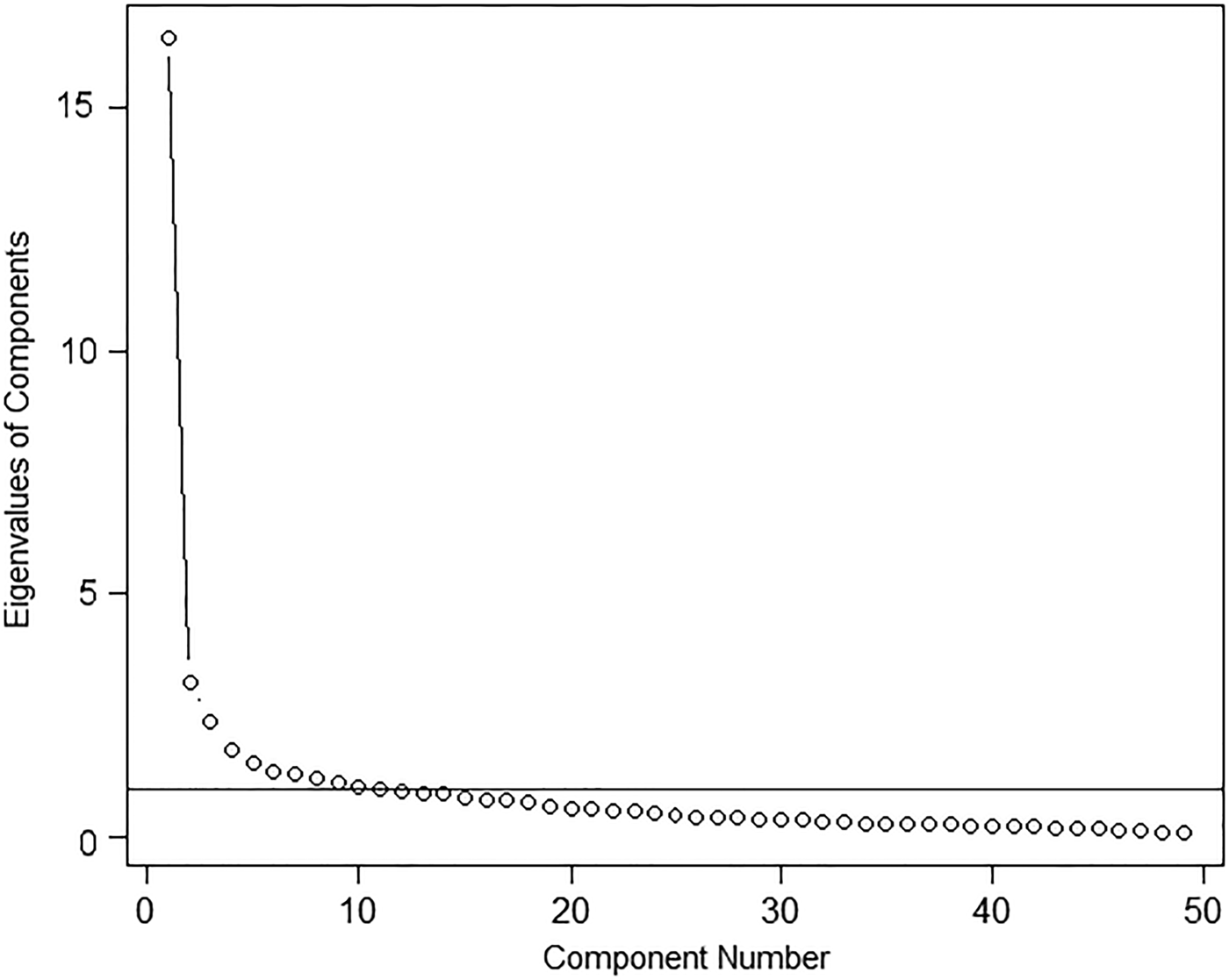
Fig. 3. Scree plot of eigenvalues for 49 crimes committed in the Philadelphia area.
Table 2. Unidimensional, two-, and three-factor solutions of 49 crimes (per 100 persons) reported by the Philadelphia Police Department

Agg, Aggravated; UFA, Uniform Firearms Act, DUI, driving under the influence of a substance.
Loadings <0.25 removed unless all loadings in that row were <0.25.
Multilevel structural equation model demonstration
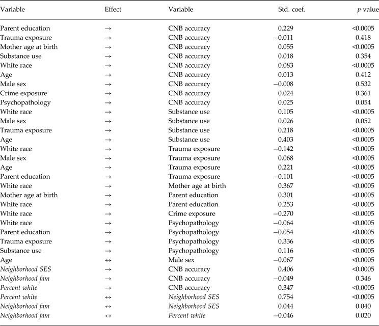
A highly complex structural model is difficult to display in graphical form; thus, Table 3 provides an example of the results of such a model predicting Computerized Neurocognitive Battery (CNB) accuracy. The first nine are direct associations of various individual-level variables with the dependent variable of interest (CNB accuracy). Further, the 27th, 28th and 29th effects listed in Table 3 are direct associations of neighborhood-level variables with CNB accuracy. All other reported associations are among the independent variables themselves. The fit of the model is acceptable (comparative fit index = 0.98; root mean square error of approximation = 0.036; standardized root mean square residual = 0.032).
Table 3. Standardized path coefficients for structural model predicting CNB accuracy across all ages, races, and genders

CNB, Computerized Neurocognitive Battery; Std. coef., standardized coefficient; Fam, family; SES, socioeconomic status.
Italics indicate variables measured at the neighborhood level; ‘→’ indicates a direct effect; ‘↔’ indicates a correlation.
The model in Table 3 is an example of a full model including age, sex, and race as covariates. Two examples of notable phenomena detailed in Table 3 are:
-
(1) The most powerful direct associations are those of parent education (individual level) and neighborhood SES (area level). The percentage of one's neighbors who are white is also a strong predictor, though it is difficult to distinguish its individual associations from those of neighborhood SES.
-
(2) Parent education mediates the association of white race with CNB accuracy. That is, the direct effect of white race on parent education is 0.253, and the direct effect of parent education on CNB accuracy is 0.229, for a combined (mediated) association of 0.253 × 0.229 = 0.058. Note that the direct association of white race with CNB accuracy is 0.083, which is only slightly larger than the mediated association. Thus, someone modeling only the direct association of white race with CNB accuracy (ignoring parent education) without considering mediating effects would acquire an incomplete picture of the overall phenomena. Indeed, the associations of other important variables (e.g. mother age at birth) in the present model make it clear that mediating effects need to be modeled. Detection of such mediations is a key strength of structural modeling of the type presented here.
Performing multiple hierarchical linear regressions for specific associations (including interactions) would indicate whether the sample should be stratified (e.g. modeling males and females separately) to further investigate the associations of demographic variables with the phenomena being modeled. Most significant interactions will suggest that stratified models are necessary.
Discussion
Previous literature corroborates our findings that individual-level socio-demographic characteristics (e.g. race and gender) of our youth participants, and aspects of their familial social capital (e.g. parental education) have statistical relationships with their neurocognitive performance (Hackman & Farah, Reference Hackman and Farah2009; Hackman et al. Reference Hackman, Farah and Meaney2010). The importance of neighborhood-level demography and crime, to further characterize the environment around these youth at the time of entry into the cohort, has also been noted (Noble et al. Reference Noble, McCandliss and Farah2007; McEwen & Gianaros, Reference McEwen and Gianaros2010). This work presents a novel conceptual approach to contextualizing neurodevelopmental assessment, in that it attempts to incorporate proximal (direct cognitive performance measurements), intermediate (individual socio-demographic and familial attributes) and distal (neighborhood-level demography) characteristics along the continuum of social determinants of health (see Warnecke et al. Reference Warnecke, Oh, Breen, Gehlert, Paskett, Tucker, Lurie, Rebbeck, Goodwin, Flack, Srinivasan, Kerner, Heurtin-Roberts, Abeles, Tyson, Patmios and Hiatt2008 for elaboration of terms).
The two factors identified utilizing exploratory factor analysis of the ACS data for our cohort study participants align with previous social epidemiology research on complex diseases. The factors highlight the importance of neighborhood-level SES, household composition, and language. Language spoken, which reflects the density of immigrants, is likely a proxy for more complex constructs that we are unable to measure without ethnographic methods (e.g. heritage-based norms, social support network dynamics that impact rearing, and acculturation).
Healthy behaviors associated with mental well-being, such as participation in the arts and physical activity, are negatively associated with crime levels (Ferreira et al. Reference Ferreira, Van Der Horst, Wendel-Vos, Kremers, Van Lenthe and Brug2007; McGinn et al. Reference McGinn, Evenson, Herring, Huston and Rodriguez2008; Lovasi et al. Reference Lovasi, Hutson, Guerra and Neckerman2009). People in crime-ridden areas are less likely to participate in healthy lifestyles and are more likely to feel stressed and depressed (Branas et al. Reference Branas, Cheney, MacDonald, Tam, Jackson and Ten Have2011). Of particular interest in our data are the strong loadings of domestic crimes (e.g. abuse and disturbance), because these crimes would likely be the most disruptive to a young person's sense of security and would likely be associated with poor mental health prognoses. Our finding that higher crime scores were associated, directly and indirectly, with lower CNB performance, is consistent with the aforementioned literature and is an important addition to our understanding of the role of social context in cognitive development.
Our multilevel models demonstrate the importance of accounting for the often complex mediating or confounding relationships between individual and neighborhood-level factors and age- and gender-related neurocognitive developmental milestones. Parental educational attainment emerges as a key example of a complex mediator of CNB performance. Our findings suggest that the developmental (household) environment created for the developing youth is a manifestation of the parents' education. The results also suggest that parental education mediates race effects, e.g. white race is associated with higher parental education and better CNB accuracy.
Further research on the resilience of those non-white youth who had high accuracy despite lower parental education may be key to developing interventions that address the need to improve parental achievement for the sake of youth cognitive development. Such interventions might also target directly involved youths whose parents have low educational attainment to supplement their environments. Parental marital status, overall household composition and maternal age at birth are linked to parental educational achievement. The temporality and directionality of those relationships require further research in this cohort. Nonetheless, these variables are associated with household SES and neighborhood composition. Neighborhood SES and composition are significant predictors of CNB performance and thus worthy targets for intervention to reduce disparities in assessment performance and improve the overall mental well-being of youth.
Acknowledgments
This work was supported by NIMH grants MH089983, MH019112, MH096891 and the Dowshen Program for Neuroscience.
Declaration of Interest
None.


