THE CHALLENGE OF A LONG-RANGE FORECAST

In forecasting, there is constant tension between two competing goals: accuracy and lead time. It makes sense that one of the key criteria on which we base our assessments of a forecast is how close its prediction matches the actual result it attempts to predict. However, as important as accuracy is how far in advance of the event of interest we can generate those predictions. A key purpose of any forecasting endeavor is to see accurately far enough into the future to reliably anticipate and prepare for future events. The key is finding the optimal balance between these two goals.

Most presidential-election forecast models have a lead time of approximately three months. The average lead time of the 11 forecasts that were featured in the 2016 PS: Political Science & Politics forecasting symposium was slightly more than three months (109.2 days) (Campbell Reference Campbell2016). The one outlier was Norpoth’s Primary Model, which generated a forecast eight months in advance of the election (246 days) (Norpoth Reference Norpoth2016).

Norpoth (Reference Norpoth2013) also has a model with an even longer lead time. His Time for Change model generates a prediction for the next election as soon as results of the current election are known, providing a four-year lead time. In 2013, Norpoth’s Time for Change model projected a 61% probability that a Republican would win the 2016 election. His Primary Model predicted that Trump had an 87% certainty of defeating Clinton (Norpoth Reference Norpoth2016).

As impressive as these lead times are, Norpoth’s models have the same shortcoming as most academic presidential-election forecast models: they generate a forecast of only the national popular-vote outcome, not the Electoral College. In that sense, Norpoth’s model was actually incorrect because Clinton won the national popular vote.

Only a model that produces state-level outcomes can generate reliable projections of Electoral College outcomes. A few recent models produce state-level predictions (Berry and Bickers Reference Berry and Bickers2012; DeSart and Holbrook Reference DeSart and Holbrook2003; Jerôme and Jerôme-Speziari Reference Jerôme and Jerôme-Speziari2016; and Klarner Reference Klarner2012). Although these models allow an extrapolation up to an Electoral College prediction, their lead times are significantly shorter than those in Norpoth’s (Reference Norpoth2016) Primary Model. The longest lead time is the Jerôme and Jerôme-Speziari model, which generates a prediction roughly five months before the election—still at least three months after Norpoth’s Primary Model. It was against this backdrop that I explored the possibility of a longer-range model that could generate both state- and national-level predictions of presidential-election outcomes (DeSart Reference DeSart2020) .

THE LONG-RANGE MODEL

Of course, one key reason why the state-level forecast models—as well as most national-level models—have lead times of only approximately three months is the availability of reliable predictor variables far in advance of the election. This creates certain structural limitations to creating longer-range forecasts of state-level outcomes. The DeSart and Holbrook (Reference DeSart and Holbrook2003) state-level model used a state-level polling variable, which is not widely available for all 50 states before September. The lack of available and reliable data for all 50 states makes it challenging to build accurate longer-range models of state-level outcomes.

With the emphasis on favoring lead time, the choices of state-level indicators so far in advance of the election were relatively limited. Therefore, national-level indicators carry much of the burden in an attempt to capture the uniform shifts that may be presented from one election to the next. My efforts ultimately resulted in a fairly parsimonious model that generates reasonably accurate forecasts a year in advance of the election. With the Democratic candidate’s share of the two-party popular vote in each state, i, in each election, j, as the dependent variable, RESULT _ij, the model uses the following four predictor variables:

RESULT_i,j-1 : This is the share of the two-party popular vote won by the Democratic candidate in each state, i, in the previous election. Pearson’s r for state-level outcomes across a one-election lag averages 0.94 for the period from 1992 to 2016, ranging from 0.91 for the 1992–1996 lag to 0.98 for the 2008–2012 lag. This establishes a baseline performance for each state.

POLLS_j : This is the average Democratic two-party share of national head-to-head polls taken 13 months in advance of the election, j. This was the real challenge and, consequently, the most important contribution to the model. I obtained data from various sources for polls conducted in October in the year before the election for each election going back to 1996. This variable is meant to capture, in part, the shift in the unique national-level context of each election year as distinct from the previous one.

Another challenge of using polling data this far in advance of the election is that the nominees for each party have not yet been determined. Therefore, polling data that pits each potential Democratic nominee against each potential Republican nominee is required as is generating a forecast for each potential matchup in a matrix. In October 2015, there were polling data for 11 possible matchups.Footnote ² Despite coming more than a year in advance of the election, this variable was highly correlated with the national-level outcome for the six elections from 1996 to 2016 (Pearson’s r=0.75).

HOME STATE_i : This is a dummy variable for each state indicating its status as a home state for each candidate, signed according to party (i.e., positive for a Democrat and negative for a Republican). However, because of the presence of the lagged RESULT variable in the model, an adjustment is made to account for the removal of the home-state advantage from the previous election. For example, the home-state “bump” that John Kerry received in Massachusetts in 2004 would no longer be present in 2008. Therefore, Massachusetts was coded 1 in 2008, in addition to Illinois being coded 1 to account for Barack Obama’s expected home-state advantage. Likewise, in addition to Arizona being coded −1 to account for John McCain’s expected boost in that state, Texas received a value of −1 to capture the loss of George W. Bush’s home-state advantage in 2004. In the case of a president running for reelection, as in 1996, 2004, and 2012, their home state receives a value of 0 to account for the fact that their advantage is already captured in the lagged RESULT variable.

CONSECUTIVE TERMS_j : This is a simple party-adjusted variable (i.e., positive for Democrats and negative for Republicans) that captures the number of terms a party has consecutively occupied the White House going into election j. Accounting for the now well-documented two-term penalty (Abramowitz Reference Abramowitz1988) in this manner captures both the impact of this effect in any given election and the removal of said effect after the previous election.

IN-SAMPLE MODEL PERFORMANCE

Regressing the RESULT variable for each of the 50 statesFootnote ³ from the six elections from 1996 to 2016 on these four predictors yields the results shown in table 1, along with various indicators of the accuracy of the model’s in-sample estimates of each election outcome. All four variables achieve statistical significance at the 0.01 level, and together they explain 89% of the variance in election outcomes in each state across the six elections.

Table 1 Long-Range Forecast Model

Notes: Dependent variable is Democratic share of the two-party popular vote in states for every election from 1996 to 2016; *p<0.05.

Note: ^† Mean absolute error.

By simply examining the point estimates for each state in each year and declaring a “winner” based on which candidate wins a majority, the model correctly “predicted” the state-level outcomes 92% of the time across the six elections. This ranges from a low of 84% in 2000 to a perfect prediction of all 50 states in 2012.

The state-level predictions then can be extrapolated to the national level for both the popular vote and the Electoral College. If we ignore the uncertainty of the model’s estimates by simply awarding each state’s electoral votes to the model’s projected popular-vote winner, we can derive a projected Electoral College outcome.

For the national popular-vote projection, the state-level predictions are weighted according to each state’s contribution to the total national popular vote in the previous election and then summed. Noteworthy is that the average absolute error of this national-level extrapolation across the six elections in the analysis is approximately 1%. In terms of specific elections, the model’s in-sample projections are remarkably close to the actual popular-vote and Electoral College outcomes in 2008 and 2012.

In the critical 2000 and 2016 elections, in which there was a discrepant outcome between the national popular-vote and Electoral College outcomes, these in-sample projections were a mixed bag. For 2000, the model correctly concluded that George W. Bush would win a majority in the Electoral College—albeit by a larger margin than he actually received—but incorrectly projected that he also would win a majority of the popular vote. The model predicted that Hillary Clinton would win razor-thin majorities in both the Electoral College and popular vote.

THE 2020 PREDICTION

Utilizing the coefficients in table 1 and entering the relevant data for each predictor variable for the current election yields the prediction shown in table 2. On average, Biden held a sizeable lead of 9.7 percentage points over Trump in the national head-to-head polls in October 2019, as reported on RealClearPolitics.com.Footnote ⁴ This translates into a projection of Biden winning 54.8% of the national two-party popular vote to Trump’s 45.2% and a majority of the Electoral College, 350 to 188.

Table 2 2020 Long-Range Forecast

Using these point estimates, along with the model’s standard error of the estimate, I generated Biden win probabilities for each state and the District of Columbia (figure 1). Most important, I highlighted the “tipping-point” state. When all states are arranged according to their respective win probabilities, this is the state that would give either candidate the necessary 270 electoral votes to win. That state is Wisconsin, which the model suggests has a 0.857 probability of being won by Biden. With all of this information, it is possible to generate confidence intervals around the model’s national-level projections by running simulated election outcomes while factoring in these probabilities. The 95% confidence intervals around both the national popular-vote and Electoral College projections in table 2 are from the distribution of 100,000 simulated elections.

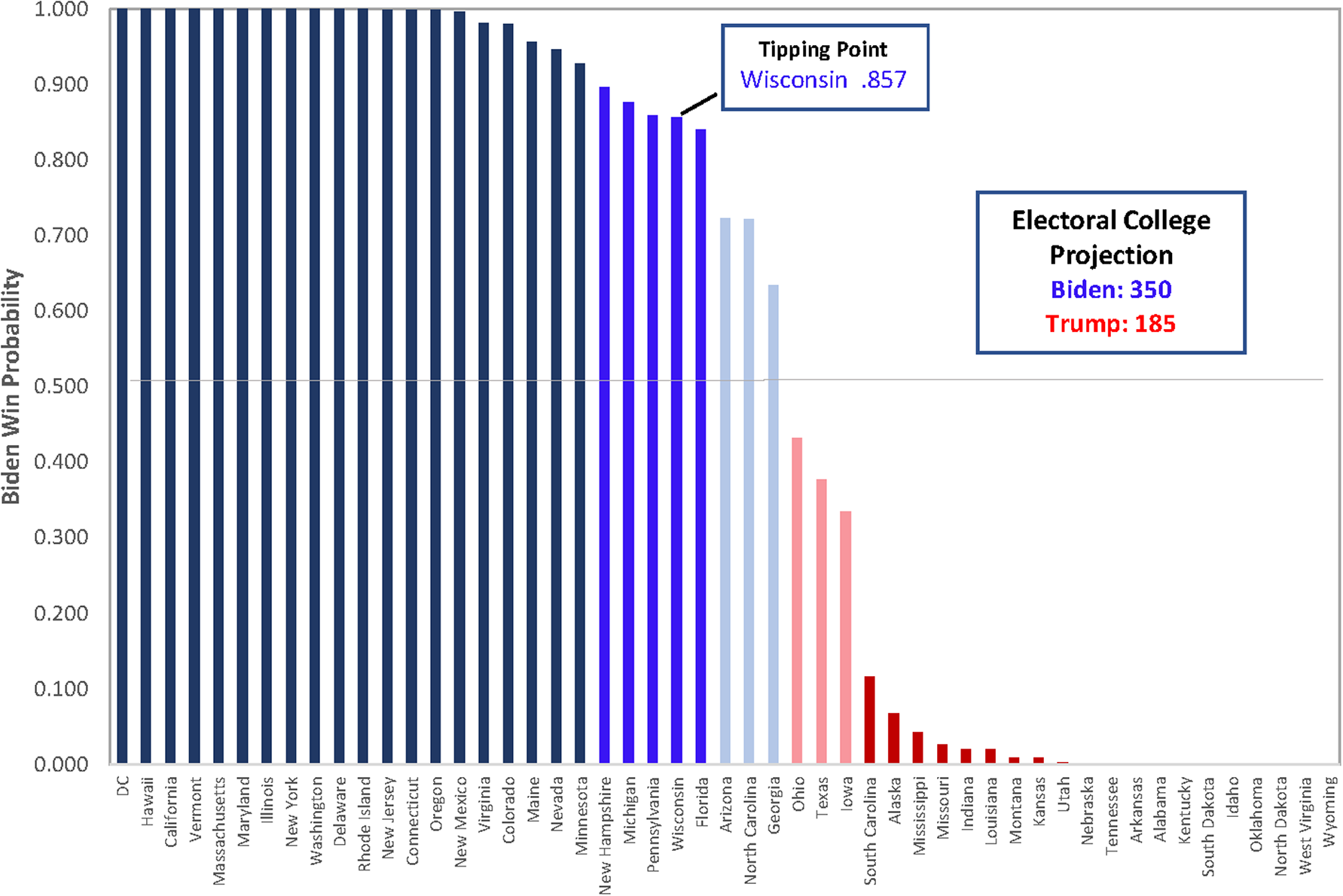
Figure 1 Long-Range Forecast Biden State-Win Probabilities

Biden won a majority of the national popular vote in every one of the simulated elections, and he won an Electoral College majority 99.85% of the time. This is largely the result of the fact that the model projects many more possible paths for Biden to get to 270 than it does for Trump. Every one of Trump’s Electoral College victories (i.e., 0.13% of the simulated outcomes) came as a result of an Electoral College misfire, just as it had in 2016. Time will tell if this is accurate or a foolhardy attempt to push the lead-time envelope.