


No CrossRef data available.
Published online by Cambridge University Press: 12 December 2005
Compared to the known univariate distributions for continuous data, there are relatively few available for discrete data. In this article, we derive a collection of 16 flexible discrete distributions by means of conditional Poisson processes. The calculations involve the use of several special functions and their properties.
Compared to the great multitude of continuous univariate distributions, there are relatively few choices available with respect to univariate discrete distributions. This is evident from the length of the compendiums of distributions available in the literature; see Johnson, Kotz, and Balakrishnan [2,3] for continuous distributions and Johnson, Kotz, and Kemp [4] for discrete distributions.
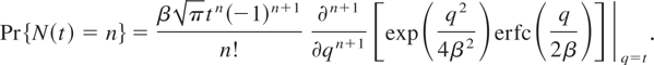
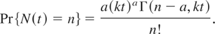
In this article, we present a collection of new discrete distributions. These are generated by means of conditional Poisson processes (Ross [6]); suppose {N(t),t ≥ 0}, where N(t) denotes the number of events during a time period of length t, is a Poisson process with rate parameter Λ. If g(λ) denotes the probability density function (p.d.f.) of Λ, then the unconditional distribution of N(t) can be written as

Now a discrete distribution for N(t) can be generated by substituting a valid form for g(λ). In this article, we generate a collection of discrete distributions for N(t) by taking g(λ) to belong to 16 flexible families. The calculations use several special functions, including the integral cosine defined by
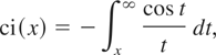
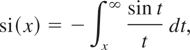
the integral sine defined by
the incomplete gamma function defined by

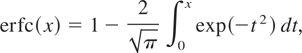
the error function defined by
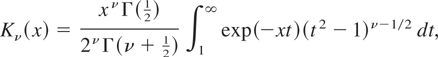
the modified Bessel function of the third kind defined by
the parabolic cylinder function defined by

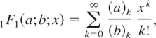
the 1F1 hypergeometric function (also known as the confluent hypergeometric function) defined by
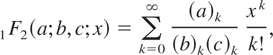
the 1F2 hypergeometric function defined by
and the Kummer function defined by

where (f)k = f (f + 1)···(f + k − 1) denotes the ascending factorial. The properties of these special functions can be found in Prudnikov, Brychkov, and Marichev [5] and Gradshteyn and Ryzhik [1].
The details of the derivation for (1) are not given in this article and can be obtained from the authors. The structural properties of N(t) are also not given since they can be obtained directly from those of Λ. For example, the mean and the variance of N(t) are
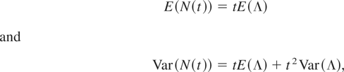
respectively. Thus, these follow directly by knowing E(Λ) and E(Λ2); see Johnson et al. [2,3].
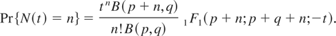
In this section, we provide a collection of formulas for Pr{N(t) = n} by taking g to belong to 16 flexible families.
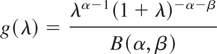
Beta distribution: If g takes the form

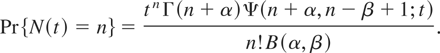
for 0 < λ < 1, then
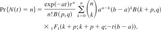
If g takes the form of the generalized beta distribution given by
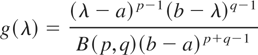
for a < λ < b, then
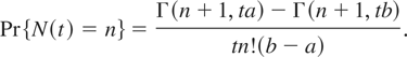
Uniform distribution: If g takes the form
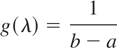
for a < λ < b, then
Inverted beta distribution: If g takes the form
for λ > 0, then
Exponential distribution: If g takes the form
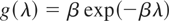
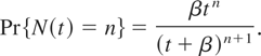
for λ > 0, then
Gamma distribution: If g takes the form
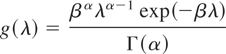
for λ > 0, then

Rayleigh distribution: If g takes the form

for λ > 0, then
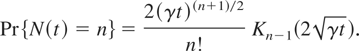
Stacy distribution (c = 2): If g takes the form
for λ > 0, then

If 2α is an integer, then the above reduces to the simpler form

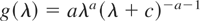
Pareto distribution of the first kind: If g takes the form
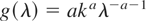
for λ > k, then
Pareto distribution of the second kind: If g takes the form
for λ > 0, then

Inverse Gaussian distribution: If g takes the form
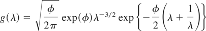
for λ > 0, then

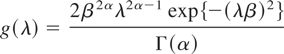
Half Normal distribution: If g takes the form
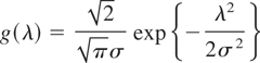
for λ > 0, then
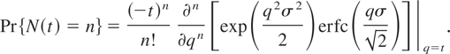
Half logistic distribution: If g takes the form
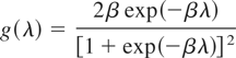
for λ > 0, then

Half Cauchy distribution: If g takes the form
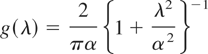
for λ > 0, then

Half t distribution: If g takes the form
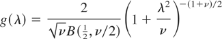
for λ > 0, then

If (1 + ν)/2 is an integer, then the above reduces to the simpler form

where
Fréchet distribution: If g takes the form
for λ > 0, then
Pearson type VI distribution: If g takes the form

for λ ≥ b > a > 0, then

We have generated a collection of 16 flexible discrete distributions. The definition of the conditional Poisson process is used as the mathematical tool. We hope that this work will help to address the inadequacy of the number of distributions available to model discrete data.
 You have
Access
You have
Access