I. INTRODUCTION
When Hugo Rietveld first developed his method for fitting powder diffraction data, it was implemented in the Algol computer language (Rietveld, Reference Rietveld1969). He shortly after rewrote that code in Fortran, which greatly facilitated its use and distribution. That Fortran code was passed from laboratory to laboratory, acquiring additional capabilities and modifications and was incorporated in many much later Rietveld refinement codes. One of the first Rietveld codes to be written completely from scratch was included in the General Structure Analysis Software (GSAS) package, which was first distributed in the early 1980s (Larson and Von Dreele, Reference Larson and Von Dreele2004). GSAS was certainly the first package that combined Rietveld analysis with other crystallographic analysis capabilities, such as fitting single-crystal data. It also provided the ability to fit to all types of diffraction data, including constant-wavelength (CW) and time-of-flight (TOF) neutron diffraction data as well as both laboratory and synchrotron powder diffraction data. GSAS pioneered many advances in the fitting of powder diffraction data, such as the combined use of multiple diffraction datasets and offered a comprehensive set of post-refinement tools.
GSAS has seen wide adoption in the crystallographic community. Use can be simplified, particularly for novice users, when combined with the EXPGUI graphical-user-interface front end (Toby, Reference Toby2001). The combination has also become a favorite platform for teaching Rietveld refinement. However, despite the successes of the GSAS/EXPGUI combination, it became clear many years ago that there are many reasons to explore creation of a new crystallographic package (Toby and Von Dreele, Reference Toby, Von Dreele and Cranswick2007). GSAS was developed within the memory limitations of computers readily available several decades ago; this now limits the ability for GSAS to handle the more complex analyses that researchers now wish. The continued support of GSAS and EXPGUI are not guaranteed. While GSAS is written in Fortran, which is presumed to be quite portable, in truth the experience shows that changes in compilers and platforms require a revalidation of the results from the code and often an extensive debugging endeavor to track down the compiler-sensitive sections of code. EXPGUI depends on the Tcl/Tk script interpreter and the unsupported BLT computational and plotting package. It has been very difficult to support this on newer operating systems. Furthermore, the target audience for the Rietveld analysis has evolved over these many years. Powder diffraction crystallographic analysis has migrated from a technique utilized by a small number of experts to one widely used in many fields for many purposes. Software needs to adapt to this, since one cannot assume the knowledge base of an expert.
For these reasons, the GSAS-II project was initiated to develop a new and modern crystallographic analysis code that expanded the scope of the original package to also include pre-refinement analysis steps such as image integration, pattern indexing, and structure solution. The GSAS-II package was previously described in the literature (Toby and Von Dreele, Reference Toby and Von Dreele2013). However, this package was not complete at the time when that was written, but it is fair to say that no actively utilized scientific package is ever completed.
GSAS-II is a graphically oriented program, both with respect to how users interact with the program, and with respect to interpretation of input and derived constants, as shown in Figure 1. GSAS-II is intended to perform all commonly needed crystallographic computations for materials crystallography as well as many needed for small-molecule and protein analysis. This includes structure solution, structure refinement, Fourier maps computation, visualization, and distance-angle computation. For powder diffraction, area detector data reduction and powder diffraction indexing routines are provided. The program will fit both single-crystal and powder data from constant wavelength X-ray and neutron sources, including laboratory instruments with both Kα1 and Kα2 radiation present. It is expected that the implementation for TOF powder and single-crystal refinement will be completed in the near future.

Figure 1. The GSAS-II user interface. GSAS-II runs with four open windows. In the case shown here, two-phase sequential fits have been made to 17 measurements made as a function of temperature. The main window (a) shows the contents of the project file as a hierarchical “tree,” which includes the parameters associated with the overall refinement, the 17 datasets and two phases. The “data display” window (b), responds to selection of a tree item in the main window and shows its contents. The third, the graphics window (c), plots results from the data display window, which in this example shows the anisotropic microstrain (residual stress) coefficients as a 3D surface. The fourth window (d) is a console (terminal) window that shows status and error messages, but is not used for any input. Note that main and data display windows have associated menu bars. For Windows and Linux, these are displayed on the windows, but for the Mac, they are displayed at the system menubar location.
It should be noted that GSAS-II is being developed in an agile fashion where new functionality is prototyped and then improved. The chosen language, Python, is particularly suited for this style of code development as well as capable of covering all aspects of the project. Code is added to the package on an on-going basis. In the ~18 months since the initial paper was written, there have been nearly 600 sets of changes to the GSAS-II codebase. Some of these changes have made mere minor spelling corrections and others represent bug fixes, but still others incorporate completely new capabilities. The goal of this paper is to outline what features have been added to GSAS-II since the previous paper was completed.
II. RIGID BODY REFINEMENT AND SIMULATED ANNEALING
The significant strength of the parent GSAS package was its pioneering flexible treatment of molecular fragments as rigid units for all scales of crystallographic refinements. This has been implemented in GSAS-II for refinements and it has been extended to structure solution. Rigid bodies are valuable in refinements where less complete data are available than what might be desired, which perhaps includes most powder diffraction analysis. Rigid bodies describe the relative arrangement of a group of atoms, but allow the orientation and location of that group of atoms to be refined. This will reduce the number of positional parameters needed to describe that group of atoms to a maximum of six and is ideal to use in refinements for materials with moieties that have very well-understood configurations, such as a perchlorate anion or a phenyl ring.
A module has also been placed into GSAS-II for solution of structures using a simulated annealing Monte Carlo fitting. In this method, atoms or molecular fragments are placed in the asymmetric unit with random locations and orientations and are then moved to improve the fit or probabilistically to sometimes degrade the fit to escape from local minima (Dmowski et al., Reference Dmowski, Toby, Egami, Subramanian, Gopalakrishnan and Sleight1988; Favre-Nicolin and Cerny, Reference Favre-Nicolin and Cerny2002; Stephens and Huq, Reference Stephens and Huq2002; David et al., Reference David, Shankland, van de Streek, Pidcock, Motherwell and Cole2006). Since the goal in structure solution is to find an approximate and possibly incomplete structural description of the material, it can be appropriate to solve the structure with idealized rigid body units, such as octahedral MO6 units, which will be modeled more accurately once the approximate structure is determined. For this process in GSAS-II, reflection intensities are estimated using Pawley refinement (Pawley, Reference Pawley1981). These intensities as well as their covariance terms are utilized in the structure solution, thus treating intensity partition for overlapped reflections as well as offering the improved speed in comparison to a full profile fit (David et al., Reference David, Shankland, van de Streek, Pidcock, Motherwell and Cole2006).
III. STATE VARIABLES, SEQUENTIAL REFINEMENT, AND PARAMETRIC FITTING
It is becoming increasingly common for researchers to collect large numbers of diffraction datasets as a function of one or more system variables, e.g. physical parameters such as temperature, chemical potential, etc. Every histogram (dataset) in GSAS-II may be labeled with five different system variables. Two of these are temperature and pressure. The other three defaults to values for humidity, applied voltage, and applied stress, but these latter three parameters can be relabeled for a project to anything that might be varied for measurement during that set of experiments.
The sequential refinement capability described in the previous GSAS-II publication has been extended for these types of analyses. In this process, an unlimited number of datasets can be read into a project and then at key points in the sequence, where there are phase changes or other changes in parameterization, manual refinements are performed. Once that is done, the sequential refinement process is started, and refinements using the remaining datasets are performed using each manually determined fit as a starting point for a group of similar datasets. The results from each successive fit can “cascade”, where the results from one refinement are used for the next, or all refinements are initiated from exactly the same parameters, or the user can designate the specific starting parameters for each fit. In GSAS-II, sequential refinements can be continued, optionally with addition of extra variables once the fit is close to a minimum, but the parameterization must be the same for each group of fits performed together. Figure 2 shows how the results from a sequential refinement may be presented.

Figure 2. The data display (a) and graphics window (b) showing output from a sequential fit of multiple datasets, as demonstrated in the sequential refinement tutorial distributed in GSAS-II.
A parametric fitting module has also been added. This is used after a sequential fit and has been performed to fit an equation of state to a refined parameter or a quantity computed from refined parameters (pseudo-variable). This equation is supplied by the user as a line of Python code and it may be non-linear and may even contain the Python “if” operator or reference user-supplied functions. The user designates which variables are free parameters and should be fit, as is shown in Figure 3. Through user-supplied functions or use of the “if” operator, different equations can be applied to different subsets of the datasets. Pseudo-variables are sets of values computed from the user-supplied function of the fit parameters. These functions are also supplied by the user, also in Python and may also be non-linear. The uncertainties for pseudo-variables are computed incorporating parameter covariance. This module thus allows for parametric fitting with proper statistical treatment, but also does so in a manner that makes it clear when the designated function is not a good fit to the equation of state, which does not happen when an equation is built into the original model as a constraint.

Figure 3. Plotting and fitting of the ratio of two lattice constants from the sequential refinement provided as a tutorial. The user-supplied equations o 1 + a 1 T k and o 2 + a 2 T are used to fit different parts of the data. The equation and fit parameters are shown in the parametric fitting window (a) and plotted in the graphics window (b). Note that the uncertainties shown for the b/c ratio are computed directly from the covariance matrix at each temperature. Uncertainties for the fitted parameters are shown in the console window (c).
IV. IMPORT AND EXPORT MODULES
Based on the experience gained with previous codes, GSAS-II uses a modular approach for reading diffraction data; when the program is started it reads in all Python files matching a specified naming convention. These files define different protocols for reading input files. A similar mechanism has now been put in place for exporting results, which include structural models (coordinates), observed and computed histograms, Fourier and charge-flipping maps, etc. from refinements. By implementing this modular approach for imports and exports, the program can be extended by the user to support new formats through the development of a short set of routines (implemented as a Python class) that can be modeled after existing code. Once this has been written, no changes are needed to GSAS-II to incorporate it into the package or place that format in appropriate menus.
Some significant import and export modules include both input and output support for the International Union of Crystallography crystallographic information framework standard (Hall et al., Reference Hall, Allen and Brown1991; Brown and McMahon, Reference Brown and McMahon2002) and the PDB format (Berman et al., Reference Berman, Westbrook, Feng, Gilliland, Bhat, Weissig, Shindyalov and Bourne2000) for protein structures. GSAS-II now can also import coordinates combined with irreducible representational modes that have been computed using the ISODISPLACE web site, http://stokes.byu.edu/isodistort.html (Campbell et al., Reference Campbell, Stokes, Tanner and Hatch2006). The modes are used to create linear constraints on the coordinates.
These import/export routines allow one to “close the loop” when using GSAS-II for the protein structure refinement in tandem with omit map creation (Bhat, Reference Bhat1988) and Coot (Emsley et al., Reference Emsley, Lohkamp, Scott and Cowtan2010) for model visualization and building.
V. UPDATING AND REGRESSION
The GSAS-II package is written in Python with a small amount of speed-sensitive coding performed in Fortran. All source code is supplied, as well as shared-library versions of the compiled Fortran code for most common computing platforms. These codes are placed in a Subversion version control system, so that every change to any part of the code is tagged with a version number (Pilato et al., Reference Pilato, Collins-Sussman and Fitzpatrick2008). If GSAS-II is installed by downloading the code directly from the Subversion repository, then a menu option can be used to check if the latest version of the code is installed. This same menu also provides an option to regress, which will return the source code to a previous version. This is provided in case an update introduces a bug or so that if there is a question, results from a previous version of the code can be compared to the results from a later version.
VI. SMALL-ANGLE SCATTERING
Capabilities for reduction analysis of isotropic small-angle scattering data have been added to GSAS-II, modeled on the Irena code (Ilavsky and Jemian, Reference Ilavsky and Jemian2009). A full description of the small-angle scattering analysis capabilities has been written (Von Dreele, in press).
VII. TUTORIALS
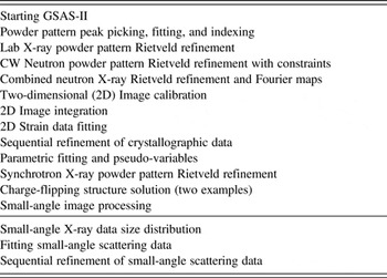
An important aspect of the documentation for GSAS-II is a set of tutorials that show how different aspects of the program are used. These tutorials are prepared as web pages that are distributed along with the source code. At present, 17 tutorials of varying length have been created. These are described in Table I.
Table I. List of currently supplied GSAS-II tutorial web pages.

VIII. SPHINX DOCUMENTATION
As GSAS-II has matured, the code has been reorganized to keep modules small and in some cases to provide better groupings for related routines. It has also grown significantly in size, although it is still much more compact than comparable ones written in other languages. To better allow developers to follow the code and locate routines, comments for most classes and higher-level routines have been provided using “restructured text”. The Sphinx documentation generator can then read these comments, which provides as output a series of web pages that include cross-referenced indices and even links showing the code (Brandl, Reference Brandl2010). The documentation from Sphinx is also available as an Adobe portable document file. This developer's documentation is expected to expand as the code does, but is currently >150 pages in length if printed.
ACKNOWLEDGEMENTS
The authors thank the many users who have taken the time to let the authors know when GSAS-II has not worked properly for them and provided the authors with enough detail to track down their problems. Many users have also provided valuable suggestions on how GSAS-II could be more useful for their work or could be more convenient; not all good suggestions have yet been followed, but in time the authors hope to get to them. Use of the Advanced Photon Source, an Office of Science User Facility operated for the US Department of Energy (DOE) Office of Science by Argonne National Laboratory, was supported by the US DOE under Contract no. DE-AC02-06CH11357.
SUPPLEMENTARY MATERIAL
The supplementary material for this article can be found at http://www.journals.cambridge.org/PDJ