II. EXPERIMENTAL

Gold films were electroplated using a BDT® 200 bath (Enthrone, Inc., New Haven, CT) with 7.5 g/L sodium thiosulfate. Films were deposited using galvanostatic conditions where the current density was 3 mA/cm². Plating times were typically ~30 min. A Ni working-electrode, Pt-mesh counter-electrode, and a saturated calomel electrode (SCE) reference-electrode were employed during the plating process. The Ni working electrode was circular with dimensions of ~15-mm diameter and ~125-μm thickness. The Au-plated film covered a circular region of ~11-mm diameter centered on the Ni electrode. Au film thicknesses for each deposition could vary between 1 and 10 μm depending on conditions of the plating bath.

Conventional θ–2θ XRD scans (a.k.a. “survey scans”) for Au films were performed using a Siemens D500 diffractometer (CuKα source, fixed slits, diffracted-beam monochromator, and scintillation detector). For subsequent texture analysis, XRD data were collected using a Bruker D8 diffractometer with GADDS (Hi-Star area detector) and an Eulerian texture cradle to obtain complete datasets in terms of 2θ, χ, and ϕ. The system employed a sealed-tube (CuKα) X-ray source with an incident-beam mirror optic (for removal of Kβ radiation). A 500-μm pinhole snout was used as an incident-beam optic to generate a small, collimated beam suitable for texture work. SLAM (Scripting Lexical Analyzer Monitor) file command protocols were generated to collect and integrate frames that covered all regions of 2θ from 15 to 80° with a χ range of 0–78° tilt, and ϕ rotation from 0 to 354° with an incremental step of 6° in χ and ϕ. The frame-series made use of four fixed 2θ positions for the area detector, while ω (i.e., θ) was scanned through an angular range of ± 7.5° on either side of 2θ/2 (the half angle of the fixed 2θ detector position) so as to necessitate a symmetric Bragg diffraction condition for every 2θ position measured in the area detector frame. The area detector 2θ positions were selected such that the 1D 2θ scans, obtained by integration of a portion of the area detector frame, would overlap. That is, the end of one 2θ scan subsequently merged to the center of the 2θ scan at the higher area detector 2θ position. A total of 3360 frames were collected for each sample. The count time for each frame was 10 s and total data collection time, including reset between frames, was 20 h (i.e., overnight).

After frame integration, the obtained 2θ scans were merged into a continuous diffraction pattern from 15 to 80°2θ, each scan having an assigned (fixed) χ and ϕ tag. This array of 2θ scans shall be referred to as “spaghetti-data” because it can be imagined as a bundle of long fibers that form a cylindrical shape, where the 2θ axis runs along the length of the cylinder. If one then views the cylinder at its top or bottom, the position of each spaghetti fiber in the bundle can be defined by polar coordinates χ and ϕ, thereby tagging each fiber to a specific location on the pole figure projection. In fact, a cross-section of a spaghetti-dataset is a pole figure for that specific 2θ position and there are as many possible individual pole figures as there are steps in the 2θ scan (typical 2θ step-size is 0.05 up to 0.1°2θ for broad peaks). The total number of diffraction patterns in the spaghetti-data bundle is the product of the χ range 0, 6, 12,…, 78° (14 steps) and the ϕ range 0, 6, 12,…, 354° (60 steps) for a total of 840 scans.

III. RESULTS AND DISCUSSION

The motivation for a detailed texture analysis of Au films was primarily to help explain apparent aberrations in Au film properties possibly linked to depletion in Au concentration in the bath. Here, we shall refer to depletion as the wt% reduction per volume of Au concentration in the BDT-200 bath as the Au metal is plated. For example, a 20% depleted sample would refer to an Au film plated from a bath that was already 20 wt% reduced in Au volume (grams/liter) prior to the plating process. For a given series of plated Au films, when each sample film is deposited sequentially Au concentration in the bath continues to be reduced (depleted). It was empirically observed that hardness of the Au films would vary and that this variability was tentatively linked to Au depletion in the bath. Fresh baths would typically generate acceptable films, but as the Au concentration decreased, film quality would decrease and ultimately fail to meet product specifications. However, just prior to the production of films that would fail film-quality criteria, a spike in properties would be observed where (most notably) the hardness of the film would change dramatically. This spike in properties might manifest at different depletion levels for a given bath and so could not be directly tied to a specific Au concentration. The perplexing nature of this result and the inability to obtain predictable process-control led to further investigation, including the texture work presented here.

As a first attempt to understand the Au-plating behavior, survey scans were performed on a representative film-series of Au-plated Ni using conventional θ–2θ XRD analysis. Figure 1 shows the resulting patterns obtained for Au films deposited from baths with different levels of Au depletion. There are several notable observations. First, the Au film deposited from the fresh bath shows an Au (111) out-of-plane preferred orientation. Other Au peaks are observed, namely (200), (220), and (311), but these peaks are small. The presence of other smaller peaks for metallic gold concurrent with a dominant (hkl) suggests that there is at least some portion of the deposited Au grains that have an approximately random out-of-plane orientation. The second observation from Figure 1 is that relative peak intensities for 20% depleted film suggest an essentially random distribution of polycrystalline gold. The integrated peak intensities for the 20% depleted Au-film were determined to be 100, 57, 31, and 39% for (111), (200), (220), and (311), respectively. These relative intensities compare very well to those of a random gold specimen: 100, 52, 32, and 36% (see PDF entry 00-004-0784; PDF, 2011). The third observation is that there is a marked difference in the 30% depleted pattern where suddenly the (220) peak becomes the dominant peak in the pattern, suggesting that (220) has now become the out-of-plane preferred orientation for the Au film. Finally, for the 40% depleted Au film, the XRD pattern returns to a more random set of relative intensities for Au. Note that Ni peaks are now observed in the 40% depleted pattern. This observation is reasonable because this Au film was substantially thinner than the other deposited films and did not show smooth Au film coverage of the Ni electrode. Prior to plotting Figure 1, the XRD patterns were normalized to the same maximum intensity scaling. However, prior to normalization, all other factors being equal, it was clear that the 40% depleted film was significantly reduced in scattering intensity. The presence of Ni peaks also confirms that the beam has penetrated through the Au film to diffract from the underlying Ni metal, whereas this was not observed in the other patterns. This is further evidence that the 40% depleted film is thinner than the others. The 40% depleted film also showed unacceptable performance in terms of adhesion to Ni. In stark contrast, the Au-film prepared using the 30% depleted bath displayed excellent properties (most notably the anomalous spike in hardness), and it seems apparent that this difference in performance is tied to the sudden change in orientation dependence of the deposited Au crystallites.

Figure 1. Survey scans for a series of Au films plated on Ni showing variation of the out-of-plane preferred orientation with Au depletion level. See text for details.

Based on the initial survey scans, it is clear that there is a major difference in terms of texture for the 30% depleted film. We focus our attention on the 30% depleted film to document the use of Tilt-A-Whirl software. This package is composed of several Matlab programs. The first program, dubbed Spaghetti-Linguine is for data formatting. The second program, called Pole-Figure-Explorer is for 2D and 3D rendering and visualization. The third program is an interactive code for data manipulation that is augmented with MVA routines. This third routine is used for applying corrections to the observed XRD data such as 2θ shift, peak intensity adjustments, and/or profile-shape reconstruction. The applied corrections may be derived from datasets collected on known standard materials or based on mathematically determined “components” extracted from a given dataset (more explanation of the term “component” will be given later). The use of each of these Matlab programs will be discussed in the context of their use as applied to the 30% depleted Au film.

The Spaghetti-Linguine program is a data processing routine that transforms the isolated XRD scans from different frame images into the 840 θ–2θ scans (spaghetti-data). In addition, this software performs a ϕ-merge of the diffraction patterns at a given χ tilt angle. For example, all 60 of the θ–2θ scans measured at χ = 12° (having ϕ = 0, 6, 12,…, 354°) are summed together to form a single pattern. The result is a set of 14 scans, each at a fixed angle in χ (0–78°) where the ϕ dimension has collapsed through summation. This ϕ-merged dataset, while losing dimensionality in the ϕ direction, can be very useful for purposes such as phase ID, scrutiny of minor phases, and initial assessment of macrostrain effects and defocus behavior. Figure 2 shows the θ–2θ scans of the ϕ-merged dataset from the 30% depleted Au film as plotted in Jade 9.0 (Materials Data, 2011). Clearly, the intensity of a given (hkl) varies widely with χ tilt, denoting significant texture effects.

Figure 2. ϕ-merged scan series for 30% depleted Au film showing intensity variation with χ tilt angle characteristic of texture. The peaks also broaden with increased χ tilt because of beam defocusing.

As mentioned earlier, intensity corrections due to defocusing errors as well as corrections for peak 2θ shift with χ (possibly due to cradle misalignment) are typically needed to obtain more representative pole figures. Our software allows corrections to be performed using two different protocols. The first correction procedure is established by the use of a powder standard which is effectively random in terms of crystallite orientation and essentially free from macrostrain. (e.g., we employed silver powder). The 2θ deviations and intensity-decay with χ tilt, derived from the analysis of the standard powder, can then be “hard-coded” into the correction-function routines that are subsequently applied to experimental spaghetti-datasets. The second correction approach is a “relative” 2θ correction of each θ–2θ scan whereby the peak positions of a given (hkl) are aligned in χ via their peak maximum, and then each peak is assigned its lost intensity (owing to defocusing) by using the information derived from a broadening function or (i.e., a broadening component). We introduce the term “component” as a reference to principal component analysis (PCA), a common form of multivariate statistical analysis that interrogates data matrixes for mathematically orthogonal parts within a large dataset, which when taken together, reflect essential pieces required to represent a given set of data, while setting aside an uncorrelated signal related to noise (Jollife, Reference Jollife2002; Rodriguez et al., Reference Rodriguez, Keenan and Nagasubramanian2007). The individual, mathematically isolated parts are referred to as components. Once these components are identified, one can attempt to assign some physical meaning to them so as to better understand the result. The broadening component is obtained by evaluation of a ϕ-merged dataset after a relative 2θ shift has brought the diffraction peaks into alignment along the χ dimension; peak alignment in χ abridges PCA of the ϕ-merged series. A point of caution is awarded here. Note that with the application of a relative 2θ correction one must also be aware that any χ dependence of the 2θ shift because of macrostrain has consequently been removed. With respect to intensity variation with χ and understanding that intensity decay of a peak is due primarily to beam defocusing, a diffraction peak will generally shrink in height but broaden in width when employing the optics present on a D8 system with area detector configuration. Hence, to first order the 2θ peak areas are usually conserved with χ tilting because what is lost in peak height is made up for in width. If one can isolate the broadening function inherent in the instrumentation, the intensity that has been smeared in 2θ because of defocusing can be reassigned through reconstruction of a given 2θ pattern. Such a pattern reconstruction is performed by first assessing representative peak profile shapes from non-broadened peaks (e.g., peak full-widths measured from a 2θ scan collected at χ = 0°). Then peaks that display broadening are redrawn based on model peak-widths; the heights of these peaks are assigned through reclamation of peak areas dictated by the PCA-derived broadening function. Just such a pattern reconstruction was performed for the 30% depleted dataset (ϕ-merged data in Figure 2). The resulting “reconstructed data” are shown in Figure 3. The detailed procedures for PCA are beyond the scope of this paper and have been documented elsewhere (e.g., Jollife, Reference Jollife2002; Van Benthem et al., Reference Van Benthem, Keenan and Haaland2002; Keenan and Kotula, Reference Keenan and Kotula2004; Rodriguez, et al., Reference Rodriguez, Keenan and Nagasubramanian2007). For brevity, isolation of the broadening function through the use of PCA augmented by multivariate curve resolution (MCR) was straightforward and easily modeled from the “relative” 2θ corrected ϕ-merged datasets.

Figure 3. ϕ-merged scan series for 30% depleted Au film after intensity correction and pattern reconstruction (see text for details).

Once a spaghetti-dataset has been generated, it may be plotted in 2D or 3D via the program Pole-Figure-Explorer. While uncorrected data may be more cumbersome to evaluate, a relatively quick assessment of texture behavior can be easily made. For example it was quickly determined, even from raw (uncorrected) spaghetti-data that the Au films displayed in-plane fiber texture. This information was of great benefit, because a lack of ϕ-dependence can serve to reduce the complexity of the dataset by collapsing the ϕ-dimension. Its benefits will be addressed later with regard to diagnosis of the texture components. Figure 4 shows the interface for the Pole-Figure-Explorer routine. The dataset employed for this figure is spaghetti-data for the 30% depleted Au film after reconstruction. In the upper-left image one can see the full dataset plotted. It has the appearance of a cylinder along 2θ axis with intensity plotted as a color variation. In fact, not all of the data are plotted. A scaled-intensity-limit slide-control has been adjusted to throw out background level counts. This greatly enhances visualization of the texture. The image in the lower-left of Figure 4 shows isolation of an individual pole figure. In this case the image represents diffracted intensity from the Au (111) planes. Pole figure isolation in 2θ is straightforward with the use of the 2θ axis-limit-control slides on the bottom of the software interface. The lower-right image in Figure 4 shows the resulting 2D pole figure generated by selection of the Spawn Pole Figure button on the interface. The generated 2D pole figure image plots the summed counts along 2θ for each χ, ϕ position. The 2θ summation is determined by the 2θ range isolated by the 2θ axis-limit controls; in this case the 2θ range was 43.7°–51.1°2θ. The images in the upper-right of Figure 4 show the 3D rendering of this Au (111) pole figure. In such 3D renderings a total of five intensity-contour-levels can be allocated and the software allows for complete spatial manipulation via the mouse or keyboard arrows. This can prove very informative when looking for subtle texture effects.

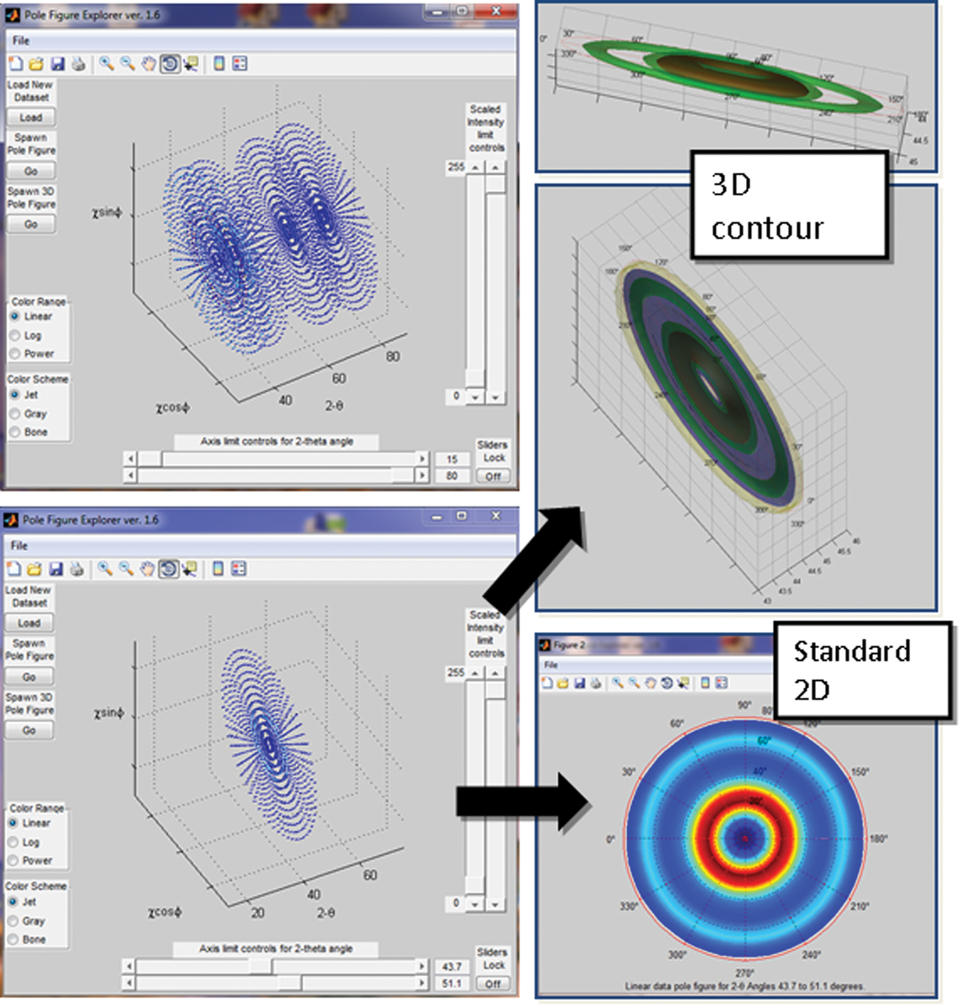
Figure 4. Examples of Pole-Figure-Explorer visualization tools using reconstructed spaghetti dataset for the 30% depleted film. Upper left: 3D rendering of complete dataset showing intensity distribution in three dimensions (χ, ϕ, 2θ). Lower left: isolated pole figure for Au (111). Lower right: resulting contour plot for the Au (111) pole figure. Upper right: 3D renderings of the Au (111) pole figure showing 2θ width dimension. Intensity is a rainbow color scale (blue = low counts, red = high counts).

As mentioned earlier, the images plotted in Figure 4 are from reconstructed spaghetti-data. However, nothing prevents the plotting of uncorrected (raw) datasets. Figure 5 shows the resulting pole figures obtained from raw spaghetti-data and reconstructed spaghetti-data. One can see that the pole figures of the raw dataset (i.e., bottom row of images in Figure 5) have more intensity variation, still, it is clear that the 30% Au depleted film has an in-plane fiber texture as indicated by the continuous rings of intensity observed in all the raw-data pole figure images. The reconstructed pole figures (middle row of images in Figure 5) have had these minor intensity variations smoothed out, so as to better observe the distinct texture of the film. Figure 5 also shows an additional option for plotting a pole figure: a 3D contour derived from a 2D pole figure where the 3D contour scales intensity as height. These 3D-height contour plots enable absolute intensity magnitude comparisons between the measured pole figures. A quick glance at the 3D-height pole figures reveals that the (111) pole figure has a clear dominance in overall scattered intensity when compared with the (220) and (311) pole figures. This is expected based on the relative intensities reported for gold (PDF, 2012). The direct comparison of relative intensity scaling is often lost in pole figures plotted as 2D color contour images because the intensity of the image is normalized to color scaling. Hence, having both methods of plotting can be useful for texture evaluation.

Figure 5. Pole figures from the 30% depleted Au film. The bottom pole figures are directly plotted from the spaghetti dataset. The middle pole figures are from the reconstructed spaghetti dataset. Pole figure intensity for the raw and reconstructed images employ a rainbow scale (blue = low counts, red = high counts). The images at the top of the figure illustrate the appearance of the reconstructed pole figures as 3D height contours that allow for absolute intensity comparison. See text for details.

After careful evaluation of the pole figures, a somewhat puzzling result was observed for the (220) pole figure. The initial observation of a strong (220) peak for the 30% depleted Au film in Figure 1 suggested a (220) out-of-plane preferred orientation. However, the (220) pole figure does not show a strong central pole of intensity at 0° χ. Instead, the intensity appears to be a “smeared” distribution of intensity from χ = 0 out to ~20° χ. This is inconsistent with the assumed (220) out-of-plane texture. There were other inconsistencies in the observed texture data when modeled in the context of a (220) out-of-plane preferred orientation. These inconsistencies are detailed in the following MVA analysis below, whose results led to a different out-of-plane preferred orientation being proposed for the 30% depleted Au film.

Based on the initial success in using PCA/MCR in isolating the broadening component of the peak profiles, it was viewed as possibly beneficial to evaluate the reconstructed data (Figure 3) with PCA/MCR methods to determine what one might extract regarding texture behavior. The major constraint employed in the attempted analysis of the reconstructed dataset was that of non-negativity (i.e., the components could not display negative intensity). This constraint is reasonable for diffraction data, can be easily implemented through MCR (Rodriguez, et al., Reference Rodriguez, Keenan and Nagasubramanian2007, Reference Rodriguez, Van Benthem, Ingersoll, Vogel and Reiche2010), and conveys a more rational solution to the oftentimes abstract nature of PCA components. The MCR results obtained from the ϕ-merged scans of the reconstructed 30% depleted Au film (i.e., Figure 3) showed a definitive four-component solution based on eigenvalue analysis. These four components are shown in Figure 6. Each component contains two descriptive parts. The first is a histogram in the 2θ dimension that looks like the typical 1D intensity vs. 2θ diffraction pattern. The counterpart of each component shows how the magnitude of the extracted 2θ scan varies in the χ dimension. The χ dependence of each component can be thought of as the deviation away from random diffraction conditions at a given χ tilt angle. Hence, a sample having a random distribution of Au crystallites would display no dependency on χ (i.e., the χ-dependence plot would be a flat line of fixed magnitude). In fact, this was exactly what was observed for the PCA/MCR analysis of the 20% depleted Au film (not shown), demonstrating the 20% depleted Au film contained a truly random grain orientation distribution. Returning to Figure 6, note that the first component (Cmpt. 1), shown in the upper-left, has a 2θ histogram dominated by the Au (111) peak and very little diffraction from the other possible Au peaks. This component has been dubbed the “(111) texture” component as it appears to isolate the (111) diffraction and assign how this scattering varies in χ. There is quite a lot of variation observed in the χ-dependence portion of Cmpt. 1. It appears that diffraction from the (111) family of planes has two maxima in χ: ~39 and ~75°. As it turns out, this component is essentially equivalent to the (111) pole figure (see Figure 5) where the ϕ dimension has collapsed. Therefore, the first component to be extracted represents necessary data required to plot the (111) pole figure, along with a very small portion of scattering of other Au peaks. If we consider the initial hypothesis of (220) out-of-plane orientation for this Au-film, one would expect only one peak maximum in the plotted χ-range and it would occur at χ = 35.3° (Cullity, Reference Cullity1978b). While one does observe a peak maximum in close proximity at χ ~39°, there is no explanation for the peak at χ ~75°.

Figure 6. PCA/MCR derived components from the reconstructed ϕ-merged data for the 30% depleted Au film. Each component consists of a 2θ and χ dependence and have been labeled based on the dominant (hkl) in the 2θ dependence portion of the component. See text details.

The second component (Cmpt. 2), shown in the upper-right in Figure 6, is dominated by the (200) family of planes. Again, there are small peaks of (220) and (311), but (200) is clearly the main focus of the component. This component shall be referred to as the “(200) texture” component and its χ-dependence shows maxima at ~25 and 65°. Note that there are angular values listed above the peaks. These will be discussed shortly. Again, one can see that just like Cmpt. 1, Cmpt. 2 is in-fact the pole figure representation with a collapsed ϕ-dimension. When evaluating Cmpt. 2 with the assumed (220) out-of-plane preferred orientation, one would expect a single peak maximum in the χ-dependence plot to occur at 45°. Instead, this location actually shows a minimum. Clearly the initial hypothesis of a (220) out-of-plane preference is wrong. A more thorough evaluation of Cmpt. 2 and possible interplanar angles indicated that if one were to assign the out-of-plane preference as the (210) family of planes (which incidentally are extinct in an FCC lattice), then the expected peak positions in the χ-dependent portion of Cmpt. 2 would occur at 26.6 and 63.4° χ. These angles match very well with our observed results. Further generation of interplanar angles shows matches for the χ-dependence of Cmpt. 1. The numeric labels shown on all the χ-dependent plots are based on a (210) out-of-plane preferred orientation. This rather unusual grain-orientation preference was difficult to diagnose because the extinct nature of the (210) in FCC meant the absence of a strong out-of-plane peak in the standard θ − 2θ scan and no means by which to view a strong out-of-plane central pole in a (210) pole figure. Instead, the texture was diagnosed based on the apparent (220) preference, when in fact the (220) planes lie tilted away from (210) by an interplanar angle of 18.4°.

Figure 7 shows the relationships between (111), (200), (220), and (311) with reference to the (210) planes. In addition, Table I lists all the expected relationships for a given set of planes when (210) lies in the plane of the film. As one can see, the values match very well with the observed χ-dependence plots for all the observed components. This is clearly demonstrated when evaluating Cmpt. 3 (see lower left of Figure 6). Cmpt. 3, dubbed the “(311) texture” component for its near exclusive (311) dependency on 2θ, shows a near perfect match to the expected peak maxima in χ as listed in Table I. For Cmpt. 4, i.e. the “(220) texture” component, one observes something a little different. The χ-dependence peaks are in more-or-less correct locations. However, it is worth noting that Cmpt 4. is not as exact in its isolation of (220) dependence with 2θ. In fact, Cmpt. 4 has a significant (311) peak present in the 2θ portion of its component. In other words, there does appear to be some correlation between the (220) and (311) planes with regard to their χ dependence and this results in some level of component mixing where the (220) component is not exclusive to the (220) texture but also has some fraction of (311) planes tied to its function. This observation is not unreasonable when considering the interplanar angles for (220) and (311) with reference to the (210) planes. It turns out that both the (220) and the (311) planes have very similar interplanar relationships, assuming a (210) out-of-plane texture preference. Consider the pairing of these interplanar angles: 18.4° vs. 19.3°, 50.8° vs. 47.6°, and 71.6° vs. 66.1° for (220) and (311) planes, respectively, when referenced to a tilt from (210) and therefore the film surface (see Table I). This close correlation probably drives the imperfect separation of some of the (311) intensity from that of the (220) in Cmpt. 4.

Figure 7. Relationship between the (210) and other observed planes in the face-centered cubic Gold lattice when the (210) plane is oriented horizontally (i.e., parallel to the film surface).

Table I. Interplanar angles for (210) out-of-plane preferred orientation.

Overall, the use of MVA to help interpret texture behavior was helpful in isolating the mathematically orthogonal components for subsequent evaluation. This rather simple example of the application of MVA to textured XRD data is shown to demonstrate proof-of-principle. In fairness, the (210) out-of-plane texture could have been derived from careful measurements of pole figures generated from the uncorrected raw data alone. However, the implications regarding extrapolation of MVA techniques to more complex texture analyses are enticing. The fact that MVA can mathematically isolate the essence of a pole figure as an individual component with minimal bias has implications for more complicated samples such as highly-textured, multi-phase unknowns where one is restricted to small specimen sizes and/or one cannot generate a more randomized powder specimen. In such cases, it may be possible to isolate the associated peaks of different phases based on the texture behavior of each observed peak. This is one of the clear benefits of a Tilt-A-Whirl spaghetti dataset.

Another useful characteristic of the spaghetti dataset is that it contains embedded macrostrain data. The inherent nature of 2θ dimensionality with χ tilt makes the measurement of in-plane biaxial strain a simple process via the ϕ-merged dataset. The benefit of ϕ-merging is that it overcomes one of the most challenging aspects of macrostrain measurement on textured samples when using the sin²ψ method (a.k.a. sin²χ). That complication results from the fact that the texture often minimizes intensities of a given (hkl) at some χ angles while making them intense at other angles. This can be even further complicated by the presence of an in-plane bi-axial texture, which adds a ϕ-dependence to the intensity distribution. Depending on what conditions of ϕ and χ one selects when making a typical macrostrain measurement, there may or may not prove to be a diffraction signal sufficient to obtain the needed d-spacing measurement with the confidence needed to assign a valid in-plane strain. Even more challenging is the added issue of beam-defocusing effects which tend to broaden peaks in 2θ as the sample is tilted in χ, thus causing additional uncertainty in the 2θ peak position. These problems can be overcome with the ϕ-merged dataset because ϕ-merging improves counting statistics and signal-to-noise for a given peak. It also allows for many different planes to be evaluated from one spaghetti dataset. One must take care not to over-apply this method for cases of tri-axial strain, and certainly the ideal peaks to investigate are those at highest 2θ, but for a simple case where an estimation of in-plane macrostrain is desired, this technique is straightforward. Figure 8 shows the resulting sin²χ plots for two Au films, the 20% depleted (which showed a random texture) and the 30% depleted film with the now identified (210) out-of-plane preferred orientation. These plots were generated from ϕ-merged datasets after they had been 2θ corrected using the “hard-coded” values from the Ag powder specimen. The use of the hard-coded correction is required because this will allow any real 2θ dependence with χ because macrostrain has to remain present in the data; whereas the “relative” shift option forces all peaks of a given (hkl) to align in χ, consequently eliminating any measureable strain. Once the ϕ-merged data were imported into JADE, it was a trivial matter to obtain the resulting plots shown in Figure 8. The plots are derived from d-spacings of the (311) reflection and show how the d-spacing changes with χ tilt. It is very interesting that the 20% depleted film showed a slightly tensile behavior, while the 30% depleted Au film was slightly compressive. It is worth noting that the absolute values of the reported strains are <0.1% and therefore considered just marginally strained when compared to an unstrained specimen. However, it does appear that these films, which differ significantly in polycrystalline orientation, also display differing properties in terms of tensile vs. compressive in-plane strain. This information, coupled with the aforementioned change in hardness for these Au films, reveals a more detailed picture of the plating process and resulting films.

Figure 8. Sin²χ plot for 20 and 30% depleted Au films showing differing macrostrain behavior for films with differing texture characteristics. The 20% depleted Au film showed a random texture and reveals a slightly tensile macrostrain, whereas the 30% depleted Au film revealed a (210) out-of-plane texture and shows a slightly compressive strain.

The detailed texture characterization of this film series was carefully investigated in the context of other films synthesized in other bath conditions. A larger picture has begun to emerge. The observed spike in hardness properties appeared to be related to the texture present in the film. Au preferred orientation dependence was similarly correlated to the nucleation models where instantaneous nucleation (fast nucleation at a small number of sites) would more probably generate random texture, but progressive nucleation (continuous nucleation at a large number of sites) would generate films with the (210) out-of-plane texture. The Au depletion level at which the spike in properties was observed was then found to correlate to the additive employed in the bath (in our case sodium thiosulfate). Therefore, conditions in the bath are affected by Au depletion levels in conjunction with additives to affect the overall nucleation behavior of Au crystallites which ultimately dictates the final properties and performance of the deposited film. Future work is focused on determining the optimum plating conditions in terms of bath chemistry so as to optimize Au film properties. An expansion of this study to include cross-sectional transmission electron microscopy (TEM) and electron back-scatter diffraction (EBSD) is being considered for verification of the obtained texture results.