I. INTRODUCTION
X-ray fluorescence (XRF) has been routinely used in various fields for quantitative elemental analysis. For accurate quantification, matrix effects should be considered and corrected. Primary X-rays produce the XRF from the objective element (element A) as well as from matrix including element B (atomic number: Z A < Z B). In this case, XRF emitted from element B could additionally produce XRF from element A. This well-known process is called secondary excitation in XRF analysis.
Recently, the confocal micro-XRF technique was developed using polycapillary X-ray lenses. This technique enables depth-selective analysis. The basic idea of confocal three dimensional (3D)-XRF was proposed in the SPIE conference proceeding (Gibson and Kumakhov, Reference Gibson and Kumakhov1993). The first confocal setup was reported with experimental data in 2000 (Ding et al., Reference Ding, Gao and Havrilla2000). The depth profiling was first demonstrated in 2003 (Kanngiesser et al., Reference Kanngiesser, Malzer and Reiche2003). After these previous papers, the research group at Osaka City University (OCU) developed a laboratory-made confocal 3D-XRF instrument. In the initial stage, two X-ray tubes were applied in confocal setup (Tsuji et al., Reference Tsuji, Nakano and Ding2007). This technique was applied to plant samples (Tsuji and Nakano, Reference Tsuji and Nakano2007), biological samples (Nakano and Tsuji, Reference Nakano and Tsuji2010), solid/liquid interfaces (Tsuji et al., Reference Tsuji, Yonehara and Nakano2008), and Japanese handicraft (Nakano and Tsuji, Reference Nakano and Tsuji2009). The research group at Atominstitut, Wien developed confocal micro-XRF having a vacuum chamber, where the sample is placed perpendicularly (Smolek et al., Reference Smolek, Pemmer, Fölser, Streli and Wobrauschek2012, Reference Smolek, Nakazawa, Tabe, Nakano, Tsuji, Streli and Wobrauschek2013). Also, OCU group developed a confocal-XRF with a vacuum chamber, where the sample is mounted horizontally (Nakazawa and Tsuji, Reference Nakazawa and Tsuji2013a).
A confocal micro-XRF has unique advantages for nondestructive depth analysis and elemental imaging at a specific depth (Schoonjans et al., Reference Schoonjans, Silversmit, Vekemans, Schmitz, Burghammer, Riekel, Brenker and Vincze2012; Tsuji and Nakano, Reference Tsuji and Nakano2011). Thus, there are many applications of this technique for layered materials; forensic samples such as car paint chips and leather samples (Nakano et al., Reference Nakano, Nishi, Otsuki, Nishiwaki and Tsuji2011), SD-memory card (Nakazawa and Tsuji, Reference Nakazawa and Tsuji2013b), and solutions (Hirano et al., Reference Hirano, Akioka, Doi, Arai and Tsuji2014). A review article on quantification of confocal micro-XRF analysis was published (Mantouvalou et al., Reference Mantouvalou, Malzer and Kanngiesser2012). Secondary enhancement was theoretically studied (Sokaras and Karydas, Reference Sokaras and Karydas2009). In this paper, secondary excitation is demonstrated using a layered sample. In addition, an analytical model for quantification of confocal micro-XRF is proposed.
II. EXPERIMENTAL SETUP
A. Confocal 3D-XRF system
The confocal 3D-XRF experimental setup used has been described elsewhere (Tsuji et al., Reference Tsuji, Yonehara and Nakano2008; Nakano and Tsuji, Reference Nakano and Tsuji2010). The sample was placed horizontally on an x–y–z translation stage. A Mo target (MCBM 50-0.6B, rtw, Germany; X-ray focus size of 50 × 50 μm) was operated at 50 kV and 0.5 mA. The X-ray tube was inclined at 45° from the horizontal plane. A polycapillary X-ray full lens was attached to the top of the X-ray tube. The spot size of the X-ray beam at the focal point was 40 μm, evaluated for the W Lα line. A silicon drift X-ray detector (SDD, X-Flash Detector, Type 1201, Bruker, Germany: sensitive area, 10 mm2; energy resolution, <150 eV at 5.9 keV) was installed with a down-looking geometry. A polycapillary X-ray half lens was attached to the end of the SDD. The spot size of the X-ray beam at the focal point was 30 μm, evaluated for the MoKα line. The energy dependence of the depth resolution in confocal micro-XRF analysis has been shown in a previous paper (Nakano and Tsuji, Reference Nakano and Tsuji2010). Typically, depth resolution was 71 μm at NiKα.
B. Layered sample
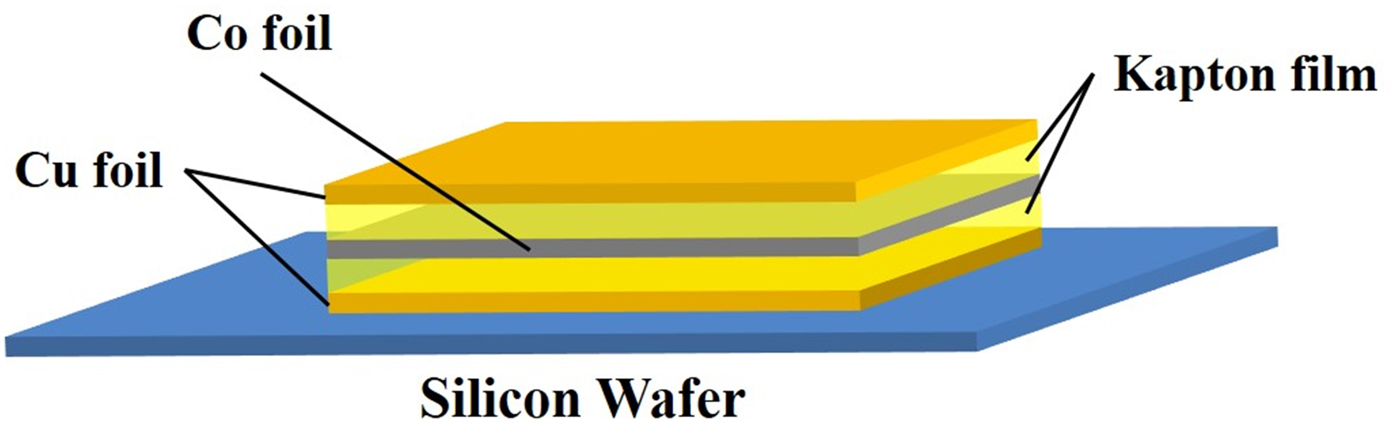
A layered sample (Cu–Co–Cu) was prepared as shown in Figure 1. Onto a Si wafer substrate, a Cu film with a thickness of 5 μm was placed. Then, a Co film (25 μm) and Cu film (5 μm) were placed. Finally, a sandwich structure sample of Cu/Co/Cu was prepared. Additionally, Kapton films were inserted between Cu/Co films and Co/Cu films as shown in Figure 1. The thickness of Kapton film was varied at 7.5, 75, and 150 μm.

Figure 1. (Color online) A sandwich structure sample: Cu film (5 μm)/Kapton/Co film (25 μm)/Kapton/Cu film (5 μm) on Si wafer.
III. RESULTS AND DISCUSSION
A. Secondary excitation process in confocal setup
A layered sample including elements A and B is assumed, where atomic number of A (Z A) is higher than that of element B (Z B); Z A > Z B. When a confocal volume is adjusted into the top layer (element A) as shown in Figures 2(a) and (b), XRF from the top layer is, of course, detected by the X-ray detector. XRF from element B in the path of the primary X-ray beam is not detectable under confocal arrangement, as shown in Figure 2(b). However, as shown in Figure 2(c), XRF emitted from the top layer (element A) can excite XRF from element B in the second layer in the path for detection. Therefore, even if the confocal volume is adjusted into the top layer (element A), additional XRF from element B can be detected under confocal arrangement due to secondary excitation effect.

Figure 2. (Color online) Possible secondary excitation in the confocal XRF arrangement for the layered sample.
Secondary excitation can also be expected when the first layer consists of element B and the second layer consists of element A. In this case, when the confocal volume is adjusted into the second layer, secondary excitation will be observed. In the process where the XRF from element A is detected, additional XRF will be produced from element B in the first layer, shown in Figure 2(d).
B. Depth profiles of layered sample by confocal micro-XRF
The sample shown in Figure 1 was measured with different thickness of Kapton film using the confocal micro-XRF instrument. The results are shown in Figure 3. Because of the approximately 71 μm depth resolution of the confocal micro XRF instrument, the depth profiles of Co (CoKα) and Cu (CuKα) were overlapped when the Kapton film was not inserted (Figure 3(a)). However, as the thickness of Kapton film increases, the profiles begin to be separated [Figures 3(b) and 3(c)]. In the case of Kapton film (thickness: 75 μm), a shoulder peak was observed on the profile of Co at a z-translation stage reading of about 500 μm, where a peak was observed for the profile of Cu. Since the confocal volume existed on the Cu layer at this depth, Co was not included in the confocal analytical volume. Therefore, it is considered that this shoulder peak of Co profile was caused by secondary excitation similar to what was shown in Figure 2(c). When the Kapton film with a thickness of 150 μm was applied, an additional peak was observed at a z-translation stage reading of about 275 μm on the depth profile of Co as shown in Figure 3(d). Since the distance between the Co layer and Cu layer was extended, two peaks of Co and Cu depth profiles were now clearly separated. This additional peak was also considered to be observed because of the secondary excitation.

Figure 3. (Color online) Depth profiles of Cu and Co by confocal micro XRF. The value of the X-axis (depth) is just reading value of z-translation stage.
The depth profiles shown in Figure 3(d) are expanded to discuss details as shown in Figure 4. As discussed before, an additional peak was observed on the Co profile at the depth (around 300 μm) marked with (2) on the left figure of Figure 4. At a z-translation stage reading of 360 μm, the confocal volume was placed into the Kapton film (thickness of 150 μm). Therefore, CuKα intensity decreased at this depth (around 360 μm) marked with (3); however, the intensity of CoKα still remained. The illustration in the right side of Figure 4 shows another mechanism of secondary excitation of confocal arrangement. Even if the confocal volume was adjusted into the Kapton layer, the primary X-rays can produce XRF of CuKα. This XRF of CuKα can produce CoKα in the beneath layer, as shown in Figure 4, leading to detection of CoKα. In any case, XRF of the element which does not exist in the confocal volume was detected by confocal micro-XRF instrument. This secondary excitation effect should be carefully considered for trace analysis by confocal micro-XRF.

Figure 4. (Color online) Left: expanded profiles of Figure 3(d). Right: possible mechanism of secondary excitation to explain the remaining Co intensity at a z-translation stage reading of 360 μm shown at (3) in the left figure.
C. Model for quantification of confocal micro-XRF
Previous discussion for secondary excitation was considered with a layered material. However, many actual samples have heterogeneous structure in plane as well as in depth. Therefore, we had to better consider the sample model of heterogeneous structure for quantification of confocal micro-XRF. Elemental mapping is performed in scanning mode with a defined step size by confocal micro-XRF. Thus, a Mosaic model shown in Figure 5 was proposed. In this model, the sample is divided in a unit cell (C ij), whose size corresponds to the confocal volume of the actual experimental setup. The step sizes in x- and z-directions are shown with dx and dz, respectively. The Mosaic model in Figure 5 is drawn in 2D. Of course, it should be drawn in 3D for 3D-XRF analysis. The confocal volume depends on the energy of XRF. Therefore, the unit cell with solid line indicates confocal volume for low energy XRF, while the cell with dotted line indicates the confocal volume for high energy XRF. We assume that the primary X-ray beam irradiates the sample with an incident angle of 45°, and that XRF is detected with an exit angle of 45°.

Figure 5. (Color online) Mosaic model for confocal micro-XRF analysis.
The following quantitative procedure is proposed neglecting secondary excitation. Chemical composition of each cell (C 11–C 14) in the first layer can be experimentally determined. In the second layer, the chemical composition of C 21– C 23 can also be determined by considering absorption in the first layer. In this way, chemical composition of all the cells can be sequentially determined from the surface top layer to the deep layers. For example, the chemical composition of C 33 is obtained after absorption correction of primary X-rays in C 12 and C 22, as well as absorption correction of XRF in C 23, C 14 cells. A calculation program will be considered in the future for quantification of confocal micro-XRF analysis for heterogeneous samples by using this Mosaic model.
IV. CONCLUSIONS
Secondary excitation process was discussed for trace analysis by confocal micro-XRF. Experimental depth profiles were shown for the layered sample of Co and Cu. An additional peak was observed and explained by secondary excitation process. The intensity of additional peak was weak, that is, the contribution of secondary excitation is not so large compared with the primary peak. However, this secondary excitation should be carefully considered in the case of analysis by confocal micro-XRF. Additionally, a Mosaic model was proposed for quantitative analysis using confocal micro-XRF.
ACKNOWLEDGMENTS
This work was supported by JSPS (Japan Society for the Promotion of Science) Grant-in-Aid for Scientific Research (B) and JSPS-FWF bilateral research project.