Nomenclature of angles

I. INTRODUCTION
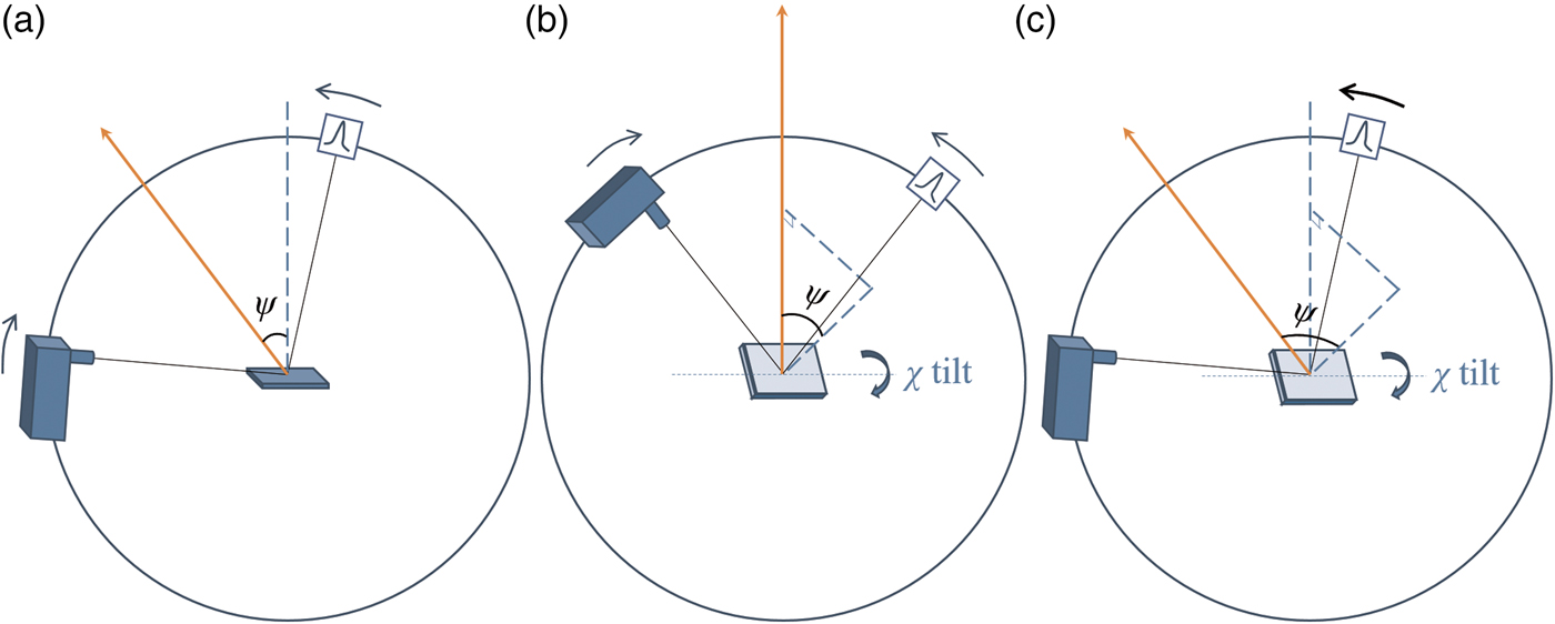
Residual stress measurement of polycrystalline bulk materials using X-ray diffraction has been extensively used in many disciplines. By measuring the d-spacing variations of crystals at different tilt angles between their crystallographic plane and sample surface, the residual stress of a bulk sample in the goniometer plane can be derived, providing the sample's Young's Modulus and Poisson ratio are known. The above tilt angle is commonly referred as the ψ angle, which can be achieved in iso-inclination mode, i.e. by an offset coupled scan [Figure 1(a)] using simultaneous movement of both the primary arm drive [Omega (ω)] and the secondary arm drive (detector). This is commonly known as the sin2 ψ method, which investigates variable information depth and works well for bulk samples. However, the sin2 ψ method is not suitable for thin-film samples, because (1) the illuminated thin-film volume decreases as the incident angle increases; (2) at certain azimuthal directions, strong single-crystal substrate peaks may over-ride thin-film reflections, invalidating some d-spacing measurements.

Figure 1. (Colour online) Geometric setups of residual stress measurements in: (a) iso-inclination mode [offset coupled scan, also known as “asymmetric Ω mode” (Genzel, Reference Genzel2005)]; (b) side inclination mode [also known as “symmetric Ψ mode” (Genzel, Reference Genzel2005)]; (c) GID method in side inclination mode (only detector is scanned). The scattering vector is labelled as an orange arrow in each geometrical setup.
Grazing incident diffraction (GID) is widely used to limit the penetration of X-rays into the surface layers. This not only increases the illuminated sample volume of thin-film layers, but also avoids reflections from the substrate. Sample and incident beam are kept stationary in GID measurements with only the detector being scanned. This means the scattering vector tilts by an angle ψ with respect to the normal of the sample surface. By measuring the full GID pattern of the polycrystalline thin film, each hkl reflection corresponds to a different ψ angle: ψ hkl = θ hkl −ω i, where θ hkl is the Bragg angle and ω i is the incident angle. The variations in d-spacing of all the hkl planes are addressed by refining an overall residual stress value. This is commonly called the “multiple-hkl” method (Marciszko et al., Reference Marciszko, Baczmański, Wróbel, Seiler, Braham, Donges, Śniechowski and Wierzbanowski2013). However, for thin-film phases in high crystallographic symmetry, often fewer hkl reflections, i.e. d-spacing values at fewer ψ tilt angles, can be measured, resulting in less reliable residual stress values.
In this case, the linkage between the crystal tilt angle ψ and the Bragg angle θ hkl needs to be separated. The side inclination mode offered by an Eulerian cradle provides a separate Chi (χ) drive to tilt the sample surface normal out of the goniometer plane [Figure 1(b)]. In this way, the crystal tilt angle ψ can be freely selected by tilting the χ drive, from 0° to that approaching 90°. If the side inclination mode is used with a symmetric coupled scan [Figure 1(b)], the crystal tilt angle ψ equals the χ angle and is not restricted by the position of the incident beam and the diffracted beam while it is in the iso-inclination mode, because the two beams form the 2θ hkl angle and both need to be above the sample surface. Despite these benefits, the information depths investigated by the side inclination mode are still variable at different χ angles. Ma et al. (Reference Ma, Huang and Chen2002) used the GID method in side inclination mode to measure thin-film residual stress, by using a point focus X-ray beam [Figure 1(c)]. This approach benefits from both grazing incidence and free selection of crystal ψ tilt. In the Ma et al. (Reference Ma, Huang and Chen2002) paper, the relationship between the crystal tilt angle ψ and the Eulerian cradle χ angle was expressed in the “direction cosine matrix”. A simpler geometric diagram is shown in this paper to highlight their relationship in an explicit analytic expression.
Perhaps the biggest drawback of the method described by Ma et al. (Reference Ma, Huang and Chen2002) (GID using side inclination mode) is the weakening of reflection intensities as the Eulerian cradle χ drive tilts to high angles, making the determination of peak positions difficult. This is because the actual incident angle is decreasing as χ increases. To overcome this drawback, an improved ω compensated GID measurement using side inclination mode is described in this paper. To ensure the azimuthal component of the incident X-ray beam remains unchanged with respect to the sample, Phi (φ) compensation is also used at the same time. This improved method was applied to a NiFe alloy thin-film sample. The relationship between the crystal tilt angle ψ and the Eulerian cradle χ angle is described geometrically and was built into TOPAS v6 Launch Mode for data analysis using parametric refinement (Stinton and Evans, Reference Stinton and Evans2007; Evans, Reference Evans2010). In addition, the construction of the TOPAS input file (.INP) is explained in detail.
II. METHODS COMPARISON AND DEVELOPMENT
A. GID measurement using side inclination mode
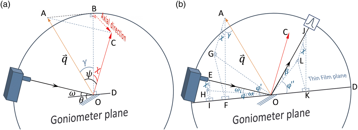
The geometric configuration of the GID method using side inclination mode (Ma et al., Reference Ma, Huang and Chen2002) is shown in Figure 2. In Figure 2(a), the scattering vector
 ${\mathop q \limits ^ \rightharpoonup}$
is in the goniometer plane OAB. The plane OAB is perpendicular to the plane OBC, in which the sample normal OC is tilted by the Eulerian cradle χ drive. With the help of the auxiliary right-angle tetrahedron OABC, the relationship between the crystal tilt angle ψ and Eulerian cradle χ angle can be derived using the Cosine Law:
${\mathop q \limits ^ \rightharpoonup}$
is in the goniometer plane OAB. The plane OAB is perpendicular to the plane OBC, in which the sample normal OC is tilted by the Eulerian cradle χ drive. With the help of the auxiliary right-angle tetrahedron OABC, the relationship between the crystal tilt angle ψ and Eulerian cradle χ angle can be derived using the Cosine Law:
 $$\cos \psi = \cos \gamma \cdot \cos \chi \; \; \; \; \; 0^\circ \le \chi \lt 90^\circ $$
As γ = θ−ω, Eq. (1) can be rewritten as:
 $$\cos \psi = \cos (\theta - \omega ) \cdot \cos \chi $$
The projections of the primary beam, the scattering vector, and the secondary beam on the thin-film surface plane are shown in Figure 2(b). It is important to note from the auxiliary tetrahedron OAGF that the azimuthal component of the scattering vector
 ${\mathop q \limits ^ \rightharpoonup} $
rotates by an angle φ’ as a result of Eulerian cradle χ tilt:
${\mathop q \limits ^ \rightharpoonup} $
rotates by an angle φ’ as a result of Eulerian cradle χ tilt:
 $$\tan \varphi ^{\prime} = \displaystyle{{\sin \chi} \over {\tan \gamma}} \; \; \; \; \; 0^\circ \le \varphi ^{\prime} \lt 90^\circ - \gamma $$
Therefore, strictly speaking this method is only suitable for thin-film samples of fibre symmetry. In fact, this method has been used on multiple azimuthal φ orientations to calculate an average residual stress for thin-film samples (Wang et al., Reference Wang, Chuang, Yu and Huang2015a, Reference Wang, Huang, Hsiao, Yu and Chenb). From Eq. (2), sin2 ψ can be represented using the known instrument drive angles θ, ω, and χ:
 $$\sin ^2\psi = \sin ^2\left( {\theta - \omega} \right) + \cos ^2\left( {\theta - \omega} \right)\sin ^2\!\!\chi $$
Substituting Eq. (4) into the common sin2 ψ method equation for residual stress measurement, results in Eq. (5) which is the same as the Eq. (10) in Ma et al. (Reference Ma, Huang and Chen2002):
 $$\eqalign{& \displaystyle{{d - d_0} \over {d_0}} = \varepsilon _{\varphi \psi} = \displaystyle{{S_2} \over 2}\sigma \cos ^2\left( {\theta - \omega} \right) \sin ^2\!\!\chi \cr & \quad + \displaystyle{{S_2} \over 2}\sigma \sin ^2\left( {\theta - \omega} \right) + 2S_1\sigma} $$
where ε φ ψ is the measured d-spacing variations, S 2/2 = (ν + 1)/E and S 1 = −ν/E are sample X-ray elastic constants, which link to the sample's Young's modulus (E) and Poisson ratio (υ). The slope of the ε φψ ~ cos2(θ − ω)sin2 χ plot is proportional to the residual stress, σ.

Figure 2. (Colour online) (a) Geometry of GID method in side inclination mode in the instrument space; the primary beam, the scattering vector OA, and the vertical line OB are in the goniometer plane; the thin-film surface normal OC is tilted out of the goniometer plane by angle χ. Note: γ = θ−ω. (b) The projections of the primary beam EO, the scattering vector OA, and the secondary beam OJ on the thin-film surface plane as HO, OG, and OL, respectively; EI, AF, and JK are in the goniometer plane and perpendicular to the Eulerian cradle χ tilt axis OD.
B. Limitation of GID in side inclination mode
Probably the biggest limitation of the original GID measurement in side inclination mode is the decrease of the actual incident angle as the Eulerian cradle χ angle increases. The geometric relationship between the actual incident angle ω i and χ angle is shown in Figure 2(b). It can be seen from the auxiliary tetrahedron OEHI that the actual incident angle ω i follows Eq. (6):
 $$\sin \omega _{\rm i} = \sin \omega \cos \chi \; \; \; \; \; \; 0^\circ \le \chi \lt 90^\circ $$
Therefore, the actual incident angle ω i is approaching 0° when the Eulerian cradle χ angle approaches 90°. For a thin-film sample of limited length, beam overspill occurs decreasing the number of X-ray photons received by the sample leading to a concomitant decrease in reflection intensity. A typical measured data set using the original GID measurement in side inclination mode is shown in Figure 3. Although the peak shift because of residual stress is obvious, the decreasing peak intensity makes the determination of peak positions at high χ angles difficult.

Figure 3. (Colour online) The measured NiFe thin-film 311 peak positions using the original GID method in side inclination mode. Peak intensity decreases as the cradle χ tilts to a high angle. The inset is a 2D plot of all the 1D patterns of different cradle χ tilts. The arrow indicates peak shift.
C. Adding ω and φ compensation to the GID in side inclination mode
It can be seen from Eq. (6) that if the actual incident angle ω i needs be kept in constant, the goniometer ω drive can be increased to compensate the Eulerian cradle χ tilt. The exact ω angle for this purpose can be calculated from Eq. (7):
 $$\eqalign{\sin \omega = \displaystyle{{\sin \omega _{\rm i}} \over {\cos \chi}} {\rm \; \; \; \; \; \; \;} 0^\circ \le \chi \le 90^\circ - \omega _{\rm i}\; \; \; \; \; \omega _{\rm i} \le \omega \le 90^\circ} $$
Practically, high χ and ω angles need to be avoided to prevent the detector moving below the OD line in Figure 2(b) (sample surface) in detector scan. It was found that χ angles up to 85° are high enough for residual stress measurement. From Eq. (7) ω is below 23° for a 2° incident angle ω i. According to Ma et al. (Reference Ma, Huang and Chen2002), a sample reflection of around 90° 2θ needs to be chosen for stress measurement, so the detector centre is well above the OD line in Figure 2(b).
It is also important to note from the auxiliary tetrahedron OEHI in Figure 2(b) that the azimuthal component of the incident X-ray beam changes by an angle φ, which increases with Eulerian cradle χ tilt:
 $$\eqalign{\sin \varphi = \tan \chi \tan \omega _{\rm i}{\rm \; \; \; \;} 0^\circ \le \chi \le 90^\circ - \omega _{\rm i}\; \; \; \; \; 0^\circ \le \varphi \le 90^\circ}$$
The Eulerian cradle φ drive can also be used to compensate for this change. Practically, when the χ angle tilts up to 85°, φ needs to be around 23° when a 2° incident angle ω i is used.
The exact ω and φ angles used to compensate the Eulerian cradle χ tilt shown in Eqs (7) and (8) guarantee a relative stationary incident beam on the thin-film surface. In this setup, the incident angle ω i is constant providing a constant illuminated thin-film volume.
In this ω–φ compensated method, the relationship between crystals tilt angle ψ and the Eulerian cradle χ angle still follows Eq. (2) and Figure 2(a), except the ω angle is now not constant:
 $$\cos \psi = \cos \left( {\theta - \omega} \right) \cdot \cos \chi $$
where ω is defined in Eq. (7). The sin2 ψ method can be written as Eq. (10):
 $$\displaystyle{{d - d_0} \over {d_0}} = \varepsilon _{\varphi \psi} = \displaystyle{{S_2} \over 2}\sigma \left[ {1 - {\cos} ^2\left( {\theta - \omega} \right){\cos} ^2\chi} \right] + 2S_1\sigma $$
Eq. (10) can be rearranged into Eq. (11), which is used to fit the d-spacing measured in this configuration.
 $$d = d_0 + d_0\sigma \left[ {\displaystyle{{1 + \nu} \over E}\left( {1 - {\cos} ^2\left( {\theta - \omega} \right){\cos} ^2\chi} \right) - \displaystyle{{2\nu} \over E}} \right] $$
III. EXPERIMENTAL
A. Instrument configurations
A Bruker D8 Advance diffractometer equipped with a Cu Kα Twist Tube set to the point focus position was used to collect GID data in side inclination mode with and without the ω–φ compensation described in Section II. A poly-capillary optics module was used to convert the diverging X-rays from the tube into a parallel beam. A collimator of 2 mm diameter was used to define the beam cross-section. A ~500 nm thick NiFe thin-film sample grown on a Si 001 substrate was mounted on a Compact Eulerian Cradle for residual stress measurement. A 0.4° equatorial soller was used to allow only parallel X-rays to reach a LynxEye XE energy-dispersive position-sensitive detector, which was operated in zero-dimensional (0D) mode [position-sensitive detectors normally can be operated in either one-dimensional (1D) mode (each channel corresponds to different 2θ angle and works independently) or 0D mode (photons counted by each channel are summed together and allocated to the 2θ angle of the centre channel, to simulate a scintillation counter)], with all the channels opened.
B. Implementation of measurement method
The measurement was planned in a .bsml file using DIFFRAC.WIZARD. The NiFe 311 reflection around 92° 2θ was scanned in GID mode with 2° incident angle and a dwell time of 2 s/step to measure the d-spacing variations at different crystal orientations. The ω and φ angles compensating Eulerian cradle χ tilts were calculated using Eqs (7) and (8) respectively, and are listed in Table I. Each row of Table I was defined as an individual method in the .bsml file, so that a single .brml result file containing 18 data ranges was generated at the end of the measurement.
Table I. The ω and φ angles to maintain a constant incident angle ω i of 2° for 18 cradle χ tilts (note φ needs to be rotated in a clockwise direction)

C. Considerations for refraction correction
With an incident angle of 2°, refraction of the primary beam is regarded as negligible. This is based on a beam deviation of only 0.02° calculated using refraction equation (12) in Genzel's (Reference Genzel2005) paper, when using 0.3° as the critical angle for the NiFe thin film with CuKα radiation. The refraction-induced deviation angle of the secondary beam is even smaller, around 0.01°, when the smallest take-off angle of the secondary beam, around 4.5°, is reached at χ = 85°. However, a refraction correction needs to be considered when the incident angle is smaller than 2°, which is summarised in Appendix. The constant incident angle guaranteed by the proposed ω–φ compensated method helps to avoid incident angles of <2° being reached, obviating the need to correct for refraction-induced X-ray beam deviations.
IV. DATA ANALYSES AND RESULTS
A. The benefit of including ω–φ compensation to the GID in side inclination mode
The resulting data acquired by using the GID in side inclination mode of the NiFe thin-film sample with and without ω–φ compensation are shown in Figures 4 and 3, respectively. The benefit of ω–φ compensation is obvious: the 311 reflection intensities at all Eulerian cradle χ tilts are almost constant. Even when the Eulerian cradle is tilted as high as 85°, the peak intensity is maintained. A slight decrease of intensity is observed because of the Eulerian cradle being tilted to a position where part of the detector window is below the sample surface. Comparing the patterns at high χ tilt angle in Figure 4 with those in Figure 3, it is clear that the peak shifts as indicated in the 2D plot in the inset of Figure 4 can be determined more reliably.

Figure 4. (Colour online) The measured NiFe thin-film 311 peak positions using the ω–φ compensated GID method in side inclination mode. Peak intensities suffer less decrease as the cradle χ tilts to a high angle. The inset is a 2D plot of all the 1D patterns of different cradle χ tilts. The arrow indicates peak shift.
B. Data analysis
The construction of the input (.INP) file for TOPAS v6 Launch Mode is shown in Figure 5. Because there is no explicit analytic solution of “2θ”, which also presents in the d-spacing, from Eq. (10), the data analysis needs be performed in two steps. Each row in steps 1 and 2 is to fit one peak using a peak phase. In step 1, the peak positions “2θ” required in Eq. (11) need to be extracted using Split Pseudo-Voigt type peak phases xo_Is. This can be realised by temporarily commenting out the refinement models in step 2. The peak positions saved in the .OUT file from the step 1 refinement can then be pasted into the “2θ” positions in step 2. The ω angles are known from Table I. The refinement of step 2 was conducted using peak phases d_Is after commenting out step1. Eq. (11) is exactly coded in the d_Is models. A single residual stress parameter “rs” (σ) was refined from all the measured d-values of NiFe 311 reflections at various Eulerian cradle χ tilts; this is considered as a parametric refinement (Stinton and Evans, Reference Stinton and Evans2007; Evans, Reference Evans2010). The refined residual stress from the data in Figure 4 is 1181 ± 85 MPa.
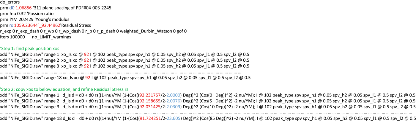
Figure 5. (Colour online) Construction of TOPAS INP file with Eq. (11) coded in step 2. The “2θ” positions in step 2 are shown in red; the ω angles in step 2 are shown in blue.
Applying the same analysis on data collected using the original method as shown in Figure 3 results in a refined residual stress of 957 ± 105 MPa. The improved method shows only slightly better refinement error because the uncertainties of peak positions extracted in step 1 was omitted when pasting them in step 2. Further development of the analysis algorithm will be able to carry the uncertainties of peak positions from step 1 to the parametric refinement of step 2 resulting in more accurate assessment of the uncertainty of the resulting residual stress. The uncertainties of peak positions extracted from the data measured using the improved method (Figure 4) are generally around 0.05°, while they are as high as 0.12° from the data measured using the original method (Figure 3). It is clear that the improved method allows more accurate peak positions to be measured.
The data analysis method can be applied to other Rietveld code, which supports parametric refinement. Otherwise the regression of ε φψ ~ [1 − cos2(θ − ω)cos2 χ] plot in Eq. (10) needs to be performed separately, after the extraction of peak positions using any profile-fitting programme.
V. CONCLUSION
The proposed compensation using ω and φ drives has been tested and shown to work well with the existing GID measurement in the side inclination mode applied to the polycrystalline thin-film residual stress measurement. The benefit of the proposed ω–φ compensation, which provides a constant incident angle, is obvious: stronger reflection intensities can be achieved at high Eulerian cradle tilt angle, which facilitates the determination of improved peak positions at high crystal tilt angle in the thin-film layer. With the realisation of constant incident angle in this improved GID measurement in side inclination mode, accurate control of thin-film information depth is possible. When the incident angle is below 2°, refraction correction is necessary. Extraction of a potential thin-film stress gradient using the proposed method warrants further exploration. Parametric refinement of a single residual stress value to simultaneously fit all the measured peak positions, as implemented here in TOPAS, allows for efficient data analysis.
ACKNOWLEDGEMENTS
The authors thank the Australian X-ray Analysis Association for the opportunity to present this work in the AXAA 2017 conference on 7 February 2017. The authors also thank Professor J.-H. Huang, National Tsing Hua University, Republic of China, for an inspiring discussion at the Thin Film 2016 conference in Singapore.
Appendix
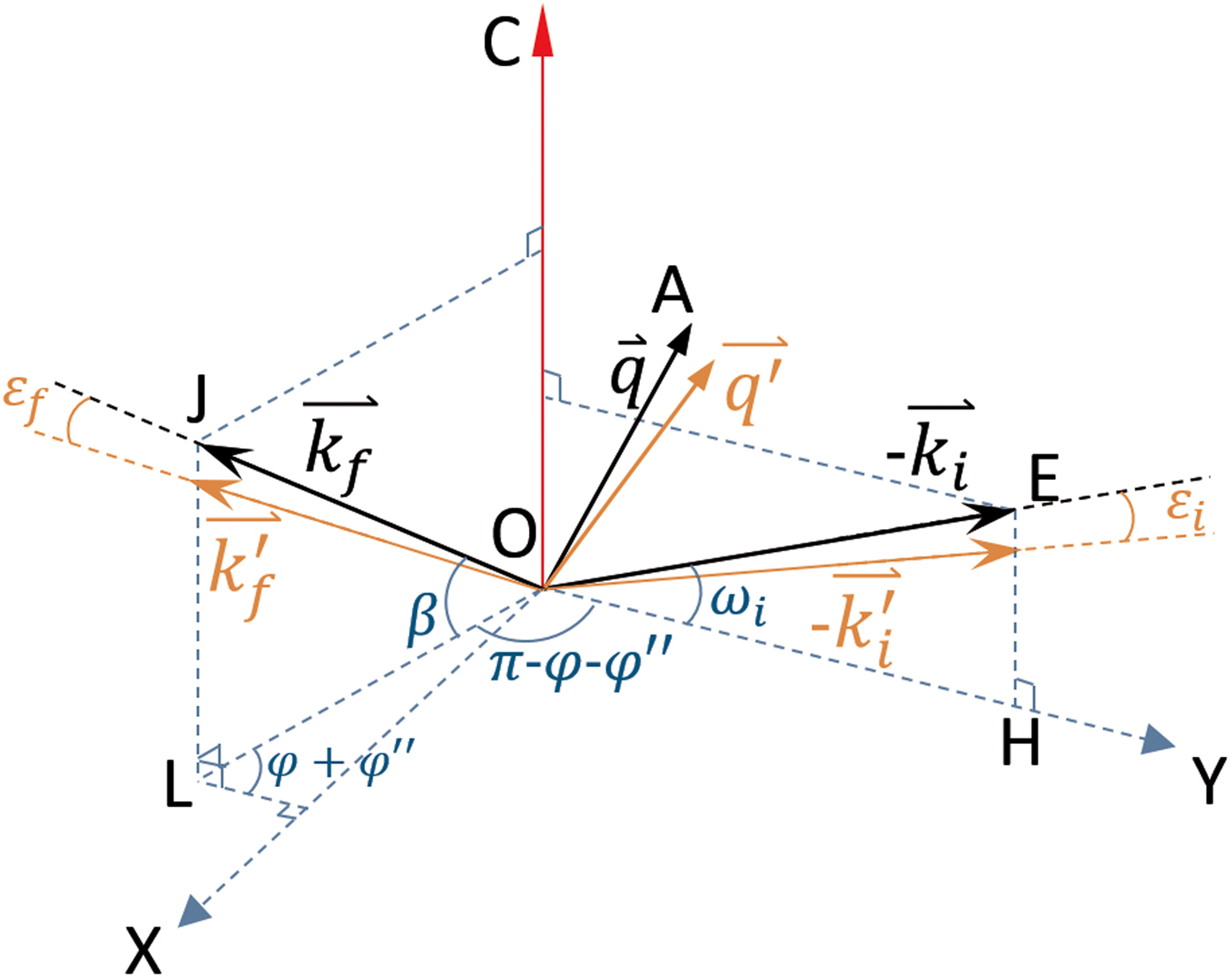
In Figure 2(b), the primary refraction plane EOH and the secondary refraction plane OJL as well as the sample normal OC are perpendicular to the thin-film surface. They are redrawn on the thin-film surface XOY plane in Figure A1, by defining OH as the y-axis. Assuming all the wave vectors
 ${\mathop k \limits ^ \rightharpoonup} $
have unity modulus, their explicit analytic expressions are:
${\mathop k \limits ^ \rightharpoonup} $
have unity modulus, their explicit analytic expressions are:
 $$\mathop{k_i}^{\rightharpoonup} = \left[ {0,\cos \omega _{\rm i},\sin \omega _{\rm i}} \right] $$
 $$ \mathop{k_i^\prime}^{\rightharpoonup} = \left[ {0,\cos \left( {\omega _{\rm i} - \varepsilon _i} \right),\sin \left( {\omega _{\rm i} - \varepsilon _i} \right)} \right] $$
 $$\mathop{k_f}^{\rightharpoonup}= \left[ {\cos \beta \sin \left( {\varphi + \varphi ^{\prime \prime}} \right), - \cos \beta \cos \left( {\varphi + \varphi ^{\prime \prime}} \right),\sin \beta} \right] $$
 $$\eqalign{\mathop {k_{f}^{\prime}}\limits^{\rightharpoonup} &= [\cos (\beta - \varepsilon _f)\sin (\varphi + \varphi ^{\prime\prime}), \cr & - \cos (\beta - \varepsilon _f)\cos (\varphi + \varphi {^{\prime\prime}}),\sin (\beta - \varepsilon _f)]} $$
where ω
i is chosen by the user, e.g. 2° in this case; φ is known from Eq. (8) for each χ angle. Analogically, β and
 $\varphi ^{\prime \prime} $
can be calculated as Eqs (A5) and (A6) from the auxiliary tetrahedron OJLK in Figure 2(b):
$\varphi ^{\prime \prime} $
can be calculated as Eqs (A5) and (A6) from the auxiliary tetrahedron OJLK in Figure 2(b):
 $$\sin \beta = \sin \left( {\pi - \omega - 2\theta} \right)\cos \chi $$
 $$\tan \varphi ^{\prime \prime} = \tan \left( {\pi - \omega - 2\theta} \right)\sin \chi $$
where ω is known from Eq. (7) for each χ angle; and 2θ are the measured peak positions.
The refraction-induced deviation angles ε i and ε f of the primary and secondary beam can be calculated from the refraction equation (12) in Genzel's (Reference Genzel2005) paper:
 $$\varepsilon = \left\{ {\matrix{ \alpha & {\alpha \lt \sqrt {2\delta}} \cr {\alpha - \sqrt {\alpha ^2 - 2\delta}} & {\sqrt {2\delta} \lt \alpha \lt x} \cr {\delta \cot \alpha} & {x \lt \alpha \lt \pi /2} \cr}} \right. $$
with x ≈ 3° · · · 5°.
The refraction-induced 2θ correction is:
 $$\Delta 2\theta = {\rm arcos}\left( {\displaystyle{{\mathop {k_f}\limits^ \rightharpoonup \cdot \left( { - \mathop {k_i}\limits^ \rightharpoonup } \right)} \over {\vert\mathop {k_f}\limits^ \rightharpoonup \vert\;\vert\mathop {k_i}\limits^ \rightharpoonup \vert}}} \right) - {\rm arcos}\left( {\displaystyle{{\mathop {k_f^{\prime} }\limits^ \rightharpoonup \cdot \left( { - \mathop {k_i^{\prime} }\limits^ \rightharpoonup} \right)} \over {\vert\mathop {k_f^{\prime} }\limits^\rightharpoonup \vert\;\vert\mathop {k_i^{\prime} }\limits^ \rightharpoonup\vert}}} \right)$$

Figure A1. (Colour online) Redrawing of the primary and secondary beams and the sample surface normal OC from Figure 2(b) on the thin-film surface XOY plane.
 ${\mathop k \limits ^ \rightharpoonup}_i $
and
${\mathop k \limits ^ \rightharpoonup}_i $
and
 ${\mathop k \limits ^ \rightharpoonup}_f $
are the measured primary and secondary vectors, respectively.
${\mathop k \limits ^ \rightharpoonup}_f $
are the measured primary and secondary vectors, respectively.
 ${\mathop k \limits ^ \rightharpoonup}_i^{\prime} $
and
${\mathop k \limits ^ \rightharpoonup}_i^{\prime} $
and
 ${\mathop k \limits ^ \rightharpoonup}_f^{\prime} $
are primary and secondary vectors after correction by refraction angles ε
i
and ε
f
, respectively.
${\mathop k \limits ^ \rightharpoonup}_f^{\prime} $
are primary and secondary vectors after correction by refraction angles ε
i
and ε
f
, respectively.
The refraction correction for crystals tilt angle ψ is:
 $$\eqalign{ \Delta \psi &= {\rm arcos}\left( {\displaystyle{{\mathop {{\rm OC}}\limits^ \rightharpoonup \cdot \mathop {q^{\prime}}\limits^ \rightharpoonup } \over {\left\vert {\mathop {{\rm OC}}\limits^ \rightharpoonup } \right\vert\;\left\vert {\mathop {q^{\prime}}\limits^ \rightharpoonup } \right\vert}}} \right) - {\rm arcos}\left( {\displaystyle{{\mathop {{\rm OC}}\limits^ \rightharpoonup \cdot \mathop {{\rm }q}\limits^ \rightharpoonup } \over {\left\vert {\mathop {{\rm OC}}\limits^ \rightharpoonup } \right\vert\;\left\vert {\mathop {{\rm }q}\limits^ \rightharpoonup } \right\vert}}} \right) \cr & = {\rm arcos}\left( {\displaystyle{{\mathop {{\rm OC}}\limits^ \rightharpoonup \cdot \left( {\mathop {k_f^{\prime} }\limits^ \rightharpoonup - \mathop {k_i^{\prime} }\limits^ \rightharpoonup } \right)} \over {\left\vert {\mathop {{\rm OC}}\limits^ \rightharpoonup } \right\vert\;\left\vert {\mathop {k_f^{\prime} }\limits^ \rightharpoonup - \mathop {k_i^{\prime} }\limits^ \rightharpoonup } \right\vert}}} \right) - {\rm arcos}\left( {\displaystyle{{\mathop {{\rm OC}}\limits^ \rightharpoonup \cdot \left( {\mathop {k_f}\limits^ \rightharpoonup - \mathop {k_i}\limits^ \rightharpoonup } \right)} \over {\left\vert {\mathop {{\rm OC}}\limits^ \rightharpoonup } \right\vert\;\left\vert {\mathop {k_f}\limits^ \rightharpoonup - \mathop {k_i}\limits^ \rightharpoonup } \right\vert}}} \right)} $$
where
 ${\mathop {\rm OC} \limits ^ \rightharpoonup} $
= [0,0,1].
${\mathop {\rm OC} \limits ^ \rightharpoonup} $
= [0,0,1].