I. INTRODUCTION
A two-dimensional X-ray diffraction (XRD2) pattern from a polycrystalline solid or powder sample can be considered as a cross-section of the detecting plane and the diffraction cones (He, Reference He2009). The conic section takes different shapes depending on the detector shape, swing angle to the direct beam, and distance from the irradiated volume in the sample. For a detector with flat detecting plane, the conic section may be an ellipse, parabola, or hyperbola. For convenience, all kinds of conic sections may be referred to as Debye diffraction rings or simply diffraction rings without referring to their specific shapes. The diffraction rings can be displayed in terms of γ and 2θ coordinates, regardless of the actual shape about the diffraction ring. The γ angle is the azimuthal angle about the incident beam and is measured along a diffraction ring in a two-dimensional (2D) pattern. Most commonly used 2D detectors have a flat detecting plane and the shape of active area can be square, rectangular, or round, determined by design or the detector technology. A flat detector has the flexibility to be used at a different sample-to-detector distance, with either high resolution at large distance or large angular coverage at a short distance.
The angular coverage of a 2D detector can be evaluated in the diffraction space as γ coverage and 2θ coverage. The γ coverage is not only determined by the detector size and distance, but also by the detector swing angle (2θ value). The 2θ coverage on the diffractometer plane is determined by the detector size and the sample-to-detector distance, regardless of the detector swing angle. Figure 1 illustrates the angular coverage of three 2D detectors with the active area of 14 × 14, 28 × 28, and 140 × 140 mm2. L is the detector width, a dimension in parallel to the diffractometer plane. The 2θ coverage (Δ2θ) on the diffractometer plane is given by:
 $$\Delta 2\theta = 2\arctan \left( {\displaystyle{L \over {2D}}} \right).$$
At 150 mm detector distance (D), the angular coverages for the three detectors are 5.3°, 10.7°, and 50°, respectively. For a detector with the rectangular active area, the detector may be oriented in a 2θ-optimized mode in which the longer dimension is aligned to the 2θ direction. The alternative is γ-optimized mode in which the longer dimension is aligned perpendicular to the diffractometer plane so as to maximize the γ coverage.
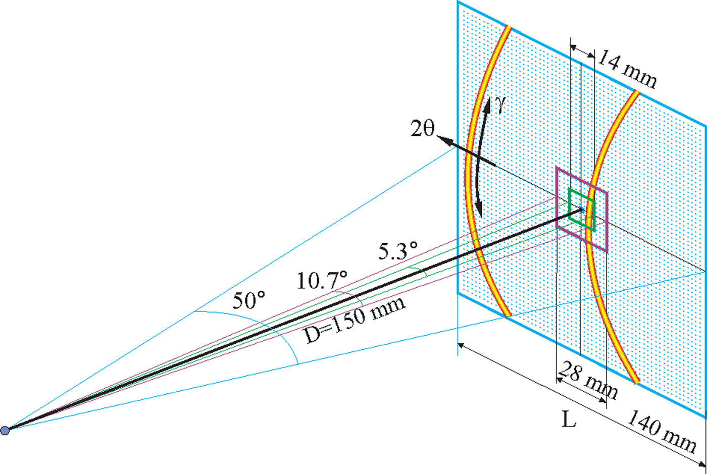
Figure 1. (Colour online) The angular coverage of 2D detectors of three different active areas.
The active area is one of the most important parameters of 2D detectors. The larger the active area of a detector is, the larger the solid angle that can be covered at the same sample-to-detector distance. This is especially important when the instrumentation or sample size forbids a short sample-to-detector distance. The sample environment chamber or special stages, such as heating stage and loading stage, may prevent short sample-to-detector distance. For instance, the data collection for in situ characterization must be able to capture the diffraction pattern corresponding to a particular stage of the phase transformation, deformation, or chemical reaction.
For many applications, it is necessary to collect a diffraction pattern with a 2θ range larger than the 2θ coverage of the available 2D detector. There are two methods to expand 2θ coverage of the collected 2D pattern if there is no change in the sample materials during the data collection. One is to collect several 2D frames at various swing angles and then merge the multiple frames to create a 2D pattern with a large 2θ coverage. The other method is to scan the 2D detector over the desired 2θ range during the data collection. For a flat 2D detector, the distance of the detector pixels to the sample varies depending on the pixel position within the 2D detector. Since the detection plane of the detector varies in orientation at different swing angles, the images collected at various swing angles cannot be simply merged or superposed to form an accurate 2D diffraction image. A smearing effect will be observed if the final 2D pattern is incorrectly constructed. In order to obtain the accurate 2D diffraction pattern within the desired 2θ range, the best strategy is to project each of the images into a cylinder detection surface so the merged or scanned diffraction pattern can be stored and displayed accurately. The following sections introduce the geometry and algorithms to project the images and to construct a 2D diffraction pattern with the expanded 2θ coverage. The position and counts of all pixels in the final 2D diffraction pattern will be as accurate as if it were collected by a detector with a cylindrical detection surface and pixels of the same size and nature. The data evaluation can then be done with the geometry and algorithms for cylindrical 2D detectors.
II. MERGE OF MULTIPLE FRAMES
The frames collected at various swing angles can be merged and displayed into one image. Figure 2(a) illustrates a 2D detector at three sequential swing angles. In order to get a continuous coverage of the merged image, the swing angle step (Δα) between two adjacent detector positions should be equal or smaller than the angular coverage (Δ2θ) of a single detector. When Δα = Δ2θ, the two adjacent detection planes meet at the edge of the detection region. In practice, to avoid the low image quality near the edge of some detectors and to get enough integration region for each frame, some overlapping between adjacent detector positions are used (Δα < Δ2θ). In this case, the adjacent detection planes intersect with an angle equal to the swing angle step (Δα). The data collected in the region outside the intersection line are redundant. The swing angle step (Δα) does not have to be equal between all adjacent detector positions but normally set as equal unless forbidden by the instrument or experimental condition.
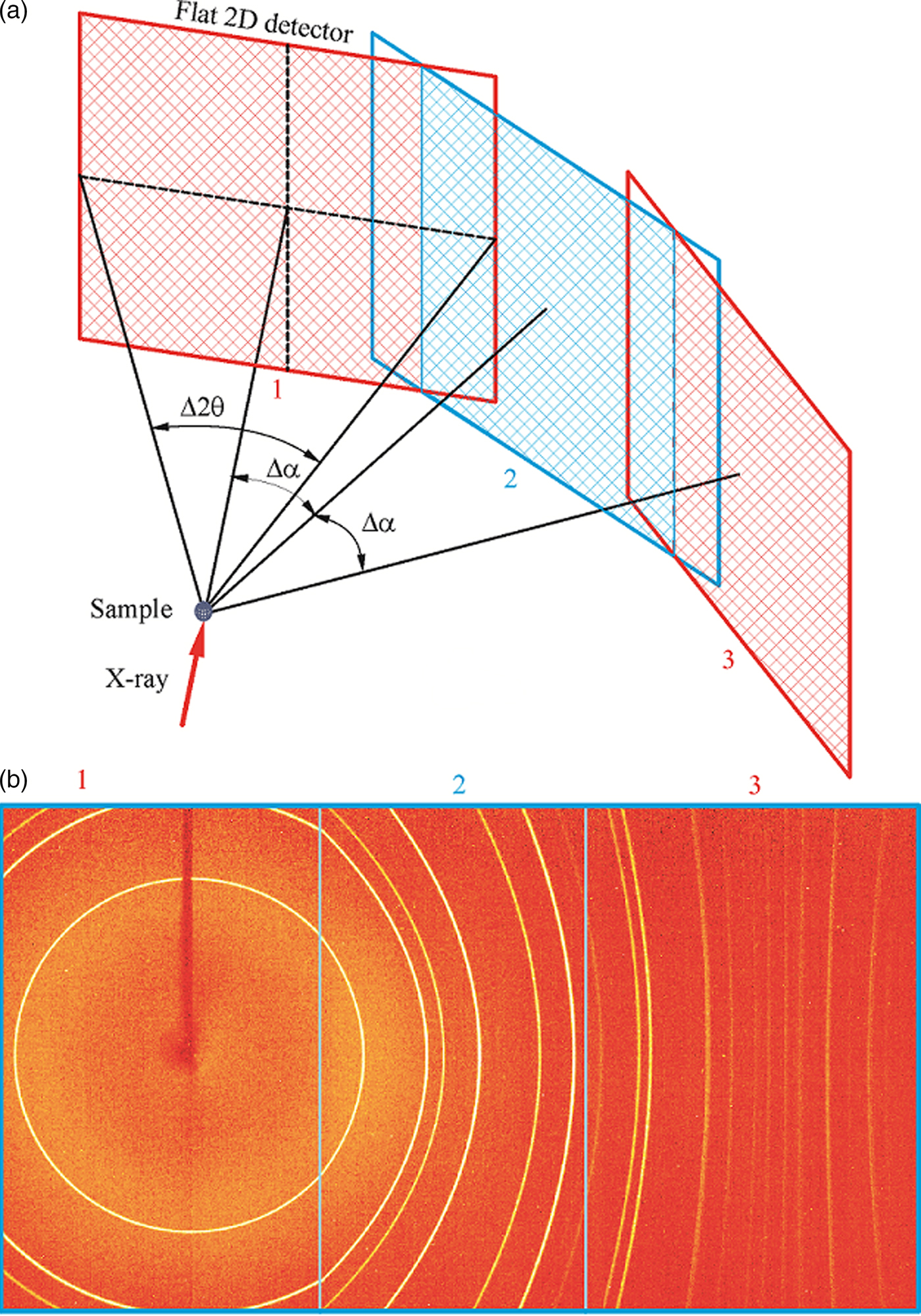
Figure 2. (Colour online) Merge of multiple frames: (a) illustration of three detector swing angles; (b) merged 2D pattern from three flat frames.
Figure 2(b) shows the merged image from the three frames collected at the above detector swing angles. The diffraction frames are collected with Bruker Photon II™ detector from 1 µm Al2O3 powder in 1 mm glass capillary at a nominal sample-to-detector distance of 9 cm. The actual sample-to-detector distance should be approximately 100.6 mm based on the active area of the detector 103.9 × 138.5 mm2. The measured angular coverage of a single frame is about 54.6°, the three frames are collected at swing angle α = 0, 40°, and 80° (Δα = 40°), respectively. In the merged image, only the region within the two intersection lines is displayed, the redundant regions outside the intersection lines are not used. The diffraction rings collected with the first frame at α = 0 are circles; the diffraction rings collected by the frames 2 and 3 may be ellipse, parabola, or hyperbola depending on the value of 2θ and α angles. A discontinuity (kink) can be observed for the diffraction rings across two diffraction frames, especially between the frames 1 and 2 when the diffraction rings have strong curvature. The merged image by the above method is mainly for display purpose. The further data integration can be done on each individual frame and then merged to produce a continuous diffraction profile. The swing angles corresponding to each of the original frames should be used for generating integration region and 2θ and γ conversion from the pixels or subpixels.
III. CYLINDER PROJECTION OF FLAT 2D FRAME
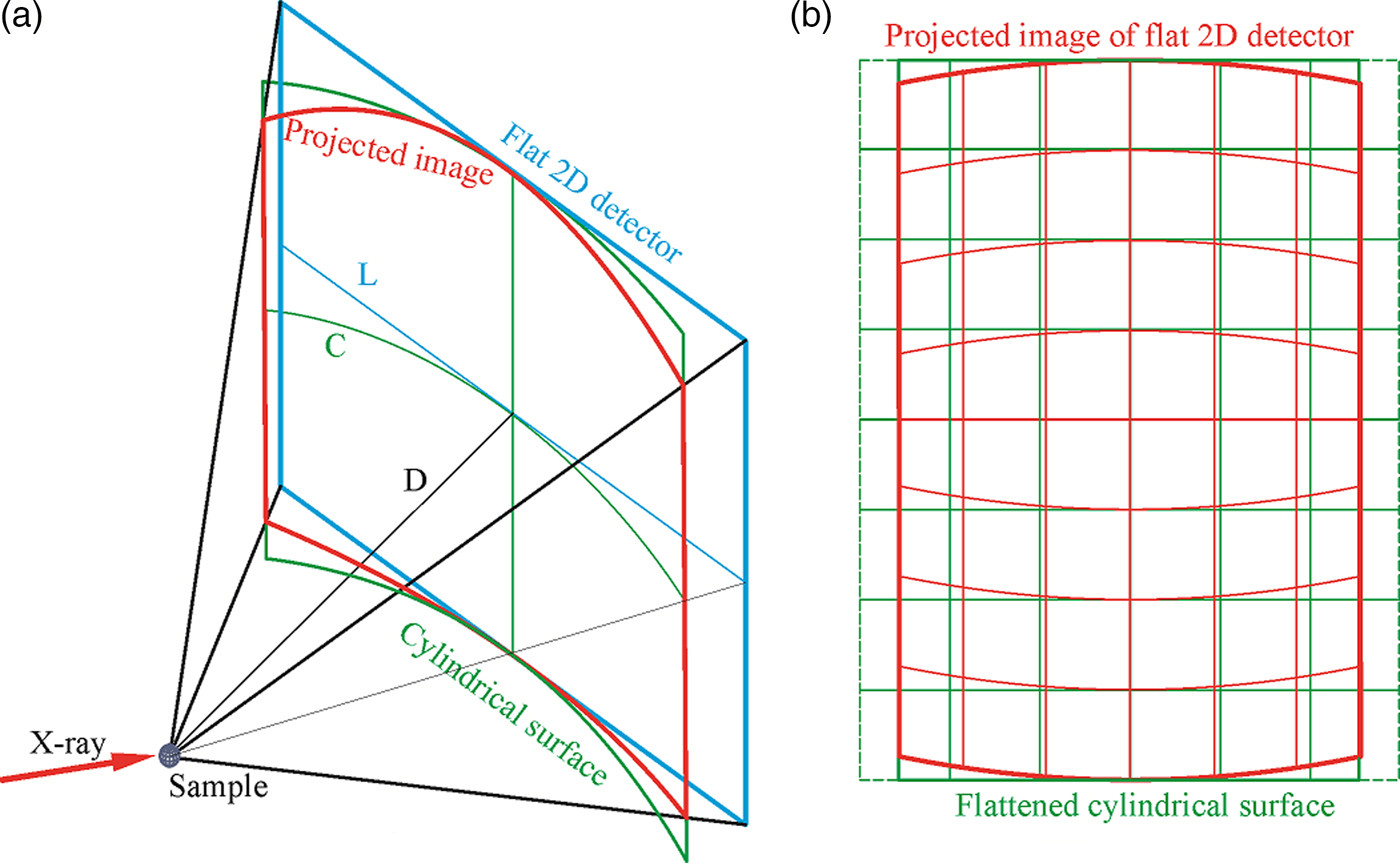
In order to accurately merge all frames collected at each detector position into a single 2D image, it is best to project all the frames to a cylindrical surface based on the scattering angle from the incident beam. As is shown in Figure 3, the position of a flat 2D detector is determined by the detector distance D and the detector swing angle α. The cross-point o is the detector center or origin of the pixel position (x, y). In the figure, three detector positions are displayed as detectors 1, 2, and 3, respectively. The detector at position 1 is set at swing angle α 1 = 0, so the detector center is on the laboratory coordinate axis X L. The detector at positions 2 and 3 is set with a swing angle step Δα, so the swing angles are α 2 = Δα and α 3 = 2Δα, respectively. The y-axis of the detector is always on the cylindrical surface at different swing angles. The radius of the cylinder is the same as the detector distance D. To merge the frames collected at all swing angles, the pixels in the flat detector are projected to the cylindrical surface through a straight line from the instrument center (sample) to the corresponding pixels. The direction of the straight line can be determined from the scattering angle given by the 2θ and γ or a different set of angles. The projected image gives the correct scattering angles for all projected pixels, and all the projected images collected at sequential detector positions fall to the same cylindrical surface. Therefore, the merged 2D image by the cylindrical projection can accurately show the diffraction rings without any distortion and discontinuity as if the diffraction pattern had been collected by a cylinder-shaped detector. Once the multiple frames are merged into a cylindrical surface, the diffraction pattern can be displayed in a flattened 2D image and evaluated without discontinuity in the conversion of the pixel position to the scattering angles 2θ and γ.
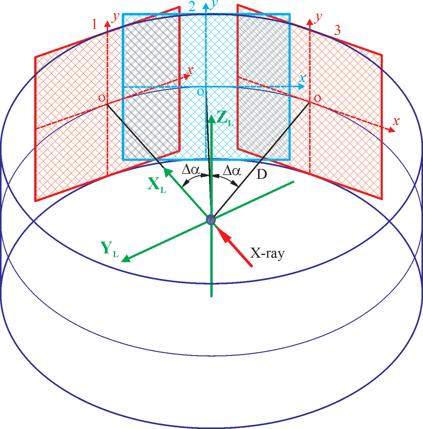
Figure 3. (Colour online) Projection of multiple frames onto a cylindrical surface.
The projection of the flat 2D detector onto the cylindrical surface introduces distortion of the detection area and pixel. Figure 4(a) illustrates the geometry of projection of a single frame onto a cylindrical surface. Assuming the image collected by the flat 2D detector is rectangular (or square) in shape, the cylindrical surface has the same height as the flat detector, the projected image onto the cylindrical surface will have the same height as the flat image in the center line (y-axis), but gradually shrinks in height away from the center line. The horizontal dimension of the flat detector is L, and the arc length of the cylindrical surface covering the same 2θ range is C. The relation between the two lengths is given by:
 $$C = D \cdot \Delta 2\theta = 2D\arctan \displaystyle{L \over {2D}}.$$
Since C is always smaller than L, so the projected image is also shrunk in the horizontal direction. Figure 4(b) illustrates the flattened surface and the projected image. Assuming the pixel shape and size in the flattened cylindrical image are the same as in the flat 2D detector, the projected pixel shape and size are also changed correspondingly as illustrated by the grid box. If the pixels in the flat 2D detector is square (or rectangular) in shape, the projected pixels are no longer square (or rectangular), and the shape and size vary depending on the position of the original pixel in the flat detector. The projected image gives the correct scattering angles for all projected pixels if treated as a cylindrical image.

Figure 4. (Colour online) Projection of single frame from a flat 2D detector onto a cylindrical surface: (a) projection geometry; (b) flattened image of the projection.
Figure 5 illustrates the geometry and algorithms to project a flat 2D image into the cylindrical surface in the laboratory coordinates. The cross-point between the X L axis and the cylindrical surface is the origin of the cylindrical surface. The image on the cylindrical surface can be displayed as a flattened image with axes u and v in rectangular coordinates. The direction of an arbitrary scattered beam S can be defined by the angle β and ρ. β is the angle between S and X L projected on the diffractometer plane X L–Y L. ρ is the angle between S and diffractometer plane. For the flat 2D detector, the scattering angle of a point P (x,y) can be given as:
 $$\rho = \arctan \displaystyle{y \over {\sqrt {x^2 + D^2}}} $$
and
 $$\beta = \alpha - \arctan \displaystyle{x \over D}.$$
For the cylindrical image, the scattering angle of a point P′(u,v) is given as:
 $${\rho} ^{\prime} = \arctan \displaystyle{v \over D}$$
and
 $${\beta} ^{\prime} = - \displaystyle{u \over D}.$$
Any point on the flat 2D detector should be projected to the point on the cylindrical surface with the same scattering angle, i.e., ρ = ρ′ and β = β′. Therefore, we can derive from the above four equations to get the following projection equation:
 $$u = D\left( {\arctan \displaystyle{x \over D} - \alpha} \right),$$
 $$v = \displaystyle{{Dy} \over {\sqrt {x^2 + D^2}}}, $$
when x = 0, u = −D α, and v = y, Eq. (7) gives the center position of the flat image relative to the cylindrical image and Eq. (8) indicates that the pixels on the y-axis projected to the cylindrical image with the same vertical position above the diffractometer plane.
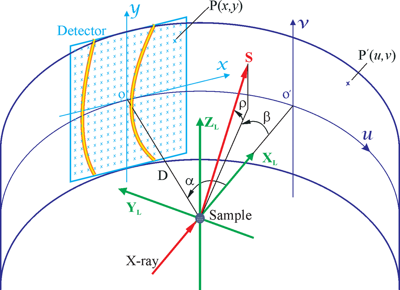
Figure 5. (Colour online) The geometry and algorithms to project a flat 2D image onto the cylindrical surface.
The above equations can be used for the pixel-to-pixel projection from the flat 2D detector into the image flattened from the cylindrical surface (cylindrical image). As is shown in Figure 6, the pixels in the flat 2D detector projected to the cylindrical image are defined by the box of red lines. The pixels in the flattened cylindrical image are defined by the box of green lines with the pixel size of Δu × Δv. Because of the projection geometry as described previously, each pixel from the flat 2D detector may contribute to several pixels in the cylindrical image. For example, the pixel P (x,y) in the flat 2D detector contributes to four pixels in the cylindrical image.
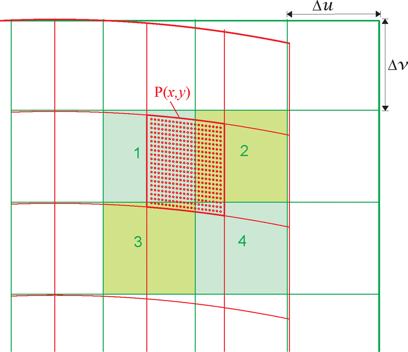
Figure 6. (Colour online) The pixel-to-pixel projection from the flat 2D image onto the flattened cylindrical image.
The direct one pixel to one-pixel projection will be too coarse to get an accurate projection. There are many methods to accurately project the pixels. For instance, the overlapping areas of the pixel P (x,y) with pixels 1, 2, 3, and 4 are calculated based on Eqs. (7) and (8). The intensity counts collected by the pixel P (x,y) can then be assigned to the pixels 1, 2, 3, and 4 proportional to the area, respectively. Calculating the contributing area for each pixel is not a programmer-friendly approach. The area of the curved pixel boundary is difficult to calculate. An alternative approach is to redistribute the counts of each pixel in the flat 2D image into a set of identical subpixels as is shown in the figure. The subpixels are discrete points evenly distributed inside the pixel area marked by circular dots. If the total number of subpixels within each pixel is M, the scattering intensity counts of each subpixel are the pixel counts divided by M. The subpixels falls into pixel 1 (dots in the upper-left region) are assigned to the pixel 1. The subpixels falls into pixel 2 (dots in the upper-right region) are assigned to pixel 2. The same is for the pixels 3 and 4. Each subpixel in the flat 2D image can be assigned to the cylindrical image pixels by Eqs. (7) and (8). The desired projection accuracy can be achieved by selecting a sufficient number of subpixels.
IV. MERGE OF OVERLAPPING REGION
The overlapping region of the frames collected by two adjacent detector swing angles can be simply ignored in the merged 2D image. However, a sharp seam line may be observed along the intersection of the two detection planes because of the inhomogeneity of scattering background or sensitivity of the certain detector. The data within the overlapping region can be treated to produce a smooth transition between adjacent frames. Figure 7(a) illustrates the flattened cylindrical image merged from two frames collected by a 2D detector with the rectangular active area. Figure 7(b) is the top view of the merged geometry. The projected images from the rectangular frames are no longer rectangular in shape. The active area of the detector is H in height and L in width. Since the y-axis is on the cylindrical surface, the vertical dimension of the projected image along the y-axis is the same as the original frame ( = 0.5H). The broken lines mark the height of the image projected from the edge of the detector:
 $$v_{\rm c} = \displaystyle{{DH} \over {\sqrt {L^2 + 4D^2}}}. $$
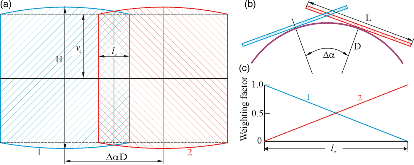
Figure 7. (Colour online) The merge of the overlapping region: (a) detector with the rectangular active area; (b) top view of two detection planes; (c) weighting factor to combine overlapping pixels.
The horizontal dimension of the overlapping region is constant from v = 0 to v c:
 $$l = D\left( {2\arctan \displaystyle{L \over {2D}} - \Delta \alpha} \right)\quad (0 \le v \lt v_{\rm c}).$$
The overlapping region beyond v c is a small arch-shaped region. In most cases, the data evaluation can be done only within the rectangular region defined by v c so that the overlapping region for v > v c can be ignored. In order to produce a smoothly merged frame, the pixels counts of both frames are combined with a weighting factor as described in Figure 7(c). Taking the case illustrated in the figure, both the flat frames are first projected to the cylindrical surface to produce the frames at left (frame 1) and right (frame 2). At any v value, the pixel of the merged image at the left end takes 100% of the pixel counts from frame 1 and 0% from frame 2. At the center of the overlapping region, the merged pixel takes 50% of pixel counts from both frames. At the right end, the merged pixel takes 100% counts from frame 2 and 0% from frame 1. By the gradual transition from frame to frame, a smoothly merged final 2D image can be created. Figure 8 shows a flattened image of the merged cylindrical frame from the same set of frames used in Figure 2(b). Based on the measured angular coverage of 54.6° for a single frame, the overlapping range covers about 14.6°. Because of smooth transition from one frame to the next, no discontinuity within the overlapping regions is observed. The final merged diffraction pattern can be used for further data evaluation as if the data had been collected by a cylindrical detector.
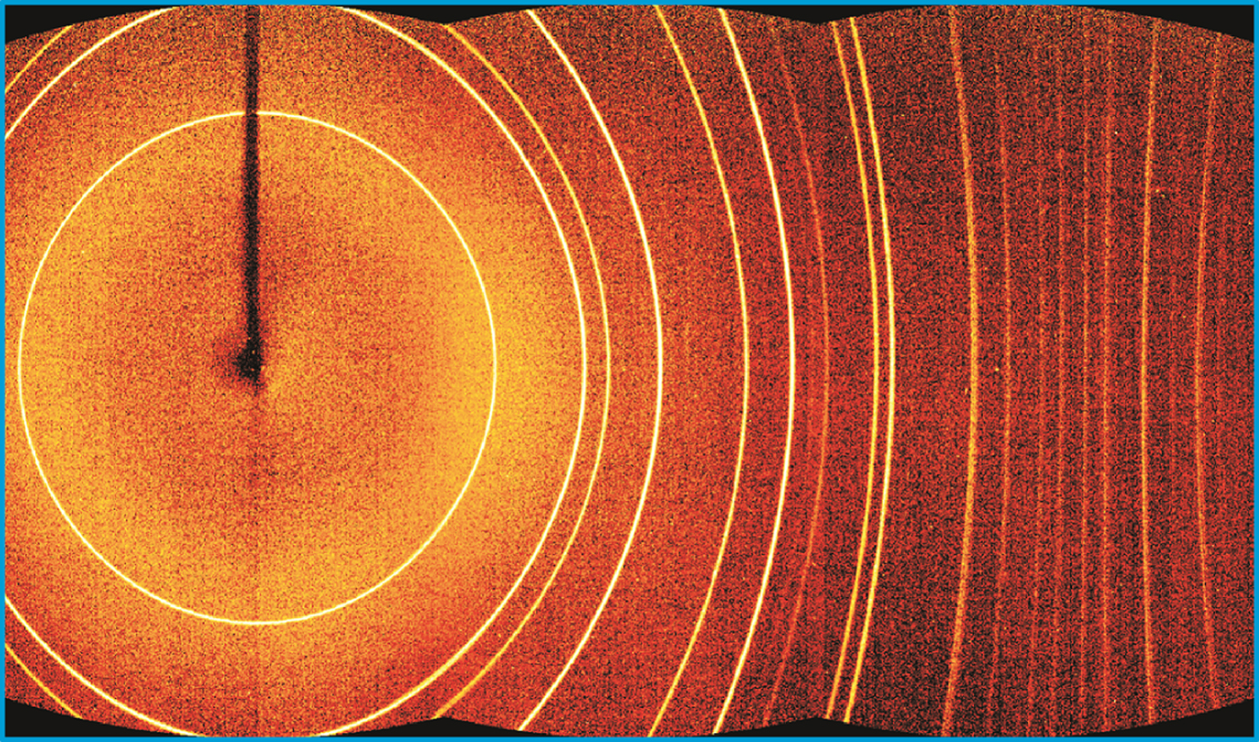
Figure 8. (Colour online) The merged image from three frames collected with Bruker Photon II™ detector from 1 µm Al2O3 powder.
V. THE 2D DETECTOR SCANNING
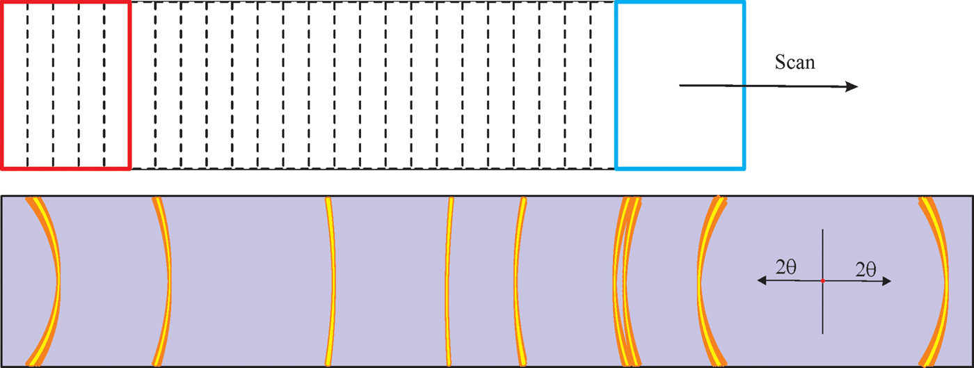
Multiple frame merge is one way to extend the angular range of a 2D detector. Another method is to scan the 2D detector over a large 2θ range. As is shown in Figure 9, a rectangular 2D detector scans over the swing angle continuously or in small steps during the data collection. The y-axis of the detector forms a cylindrical surface during the data collection scan. The radius of the cylinder is the sample-to-detector distance (D). The edge of the detector forms another cylindrical surface with a radius of E. The trace of all the pixels of the scanning 2D detector falls in the gap between two cylindrical surfaces. Because of the variable pixel-to-sample distance and variable solid angle covered by different pixel at different detector position, if the frames collected at sequential detector positions are simply superposed from the original rectangular frames, the smearing effect will be produced to the diffraction ring as illustrated in Figure 10.
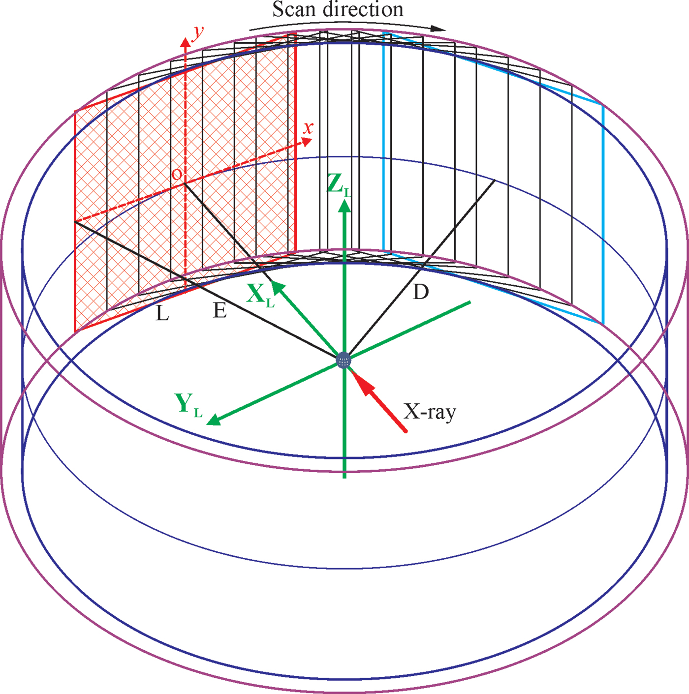
Figure 9. (Colour online) The 2D detector scans along the detection circle while collecting diffraction signals.

Figure 10. (Colour online) Smearing effect when the sequential 2D frames are simply superposed from the original rectangular frames.
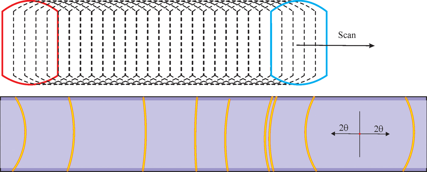
In order to accurately add all frames collected at each detector position to a single 2D image, it is best to project all the frames to the cylindrical surface based on the scattering angle from the incident beam (He et al., Reference He, Meding, Maurer and Olinger2015). The same algorithms for the multiple frames merge onto a cylindrical image in the previous section can be used to produce the scanned 2D image. The projected image gives the correct scattering angles for all projected pixels and all the projected images collected at sequential detector positions falls to the same cylindrical surface. Therefore, the scanned image by superposition of the cylindrical projections can accurately show the diffraction rings without smearing effect as illustrated in Figure 11. On top and bottom of the final scanned image, there are regions with reduced total exposure time because of the arch shape of the projected image. The pixel counts in this region can be either normalized or ignored. The final scanned diffraction pattern can be used for further data evaluation as if the data had been collected by a cylindrical detector.

Figure 11. (Colour online) Accurate diffraction rings without smearing effect when the cylindrical projections from sequential 2D frames are combined.
As seen from Figure 11, there is a ramping up region at the left side and ramping down region at the right side in terms of the exposure time. In order to collect a 2D diffraction pattern with consistent counting statistics, it is necessary to collect the diffraction pattern with homogenous exposure time over the desired 2θ range. The common practice is to start the scanning with an under travel equivalent to the angular coverage of the 2D detector (Δ2θ), and finish the scanning with an over travel of the same range. Since the swing angle (α) of the 2D detector is based on the center of the detector, the actual start swing angle (α 1) has an offset of Δ2θ/2 below the starting 2θ position and the finish swing angle (α 2) with the same offset above the end 2θ position. If the instrument condition or experiment do not allow the under and/or over travel of the detector, the final image should be normalized against the exposure time or another strategy to produce a 2D pattern with homogeneous exposure time (He, Reference He2017).
Scanning 2D detector is especially suitable for collecting a 2D pattern of large 2θ range with a small 2D detector or a rectangular detector in γ-optimized mode. Figure 12 shows a 2D image collected by scanning a DECTRIS EIGER2™-R-500 K 2D detector in γ-optimized mode covering all diffraction rings within the 2θ range of 20–80° at a detector distance of 150 mm. The region within the box of blue-dotted line corresponds to the coverage of a single frame. The 2D diffraction pattern is obtained by integration from consecutive flat 2D frames with scanning step of 0.02°. Because of the accurate projection in subpixel level, there is no smearing effect. The vertical dimension is about 70 mm after the region with reduced exposure time near the top and bottom regions are removed. The regions covered by the under and over travel are also removed. The final 2D image is as accurate as if the image had been collected with a cylindrical detector of 70 × 157 mm2 (arc length) with a radius of 150 mm.
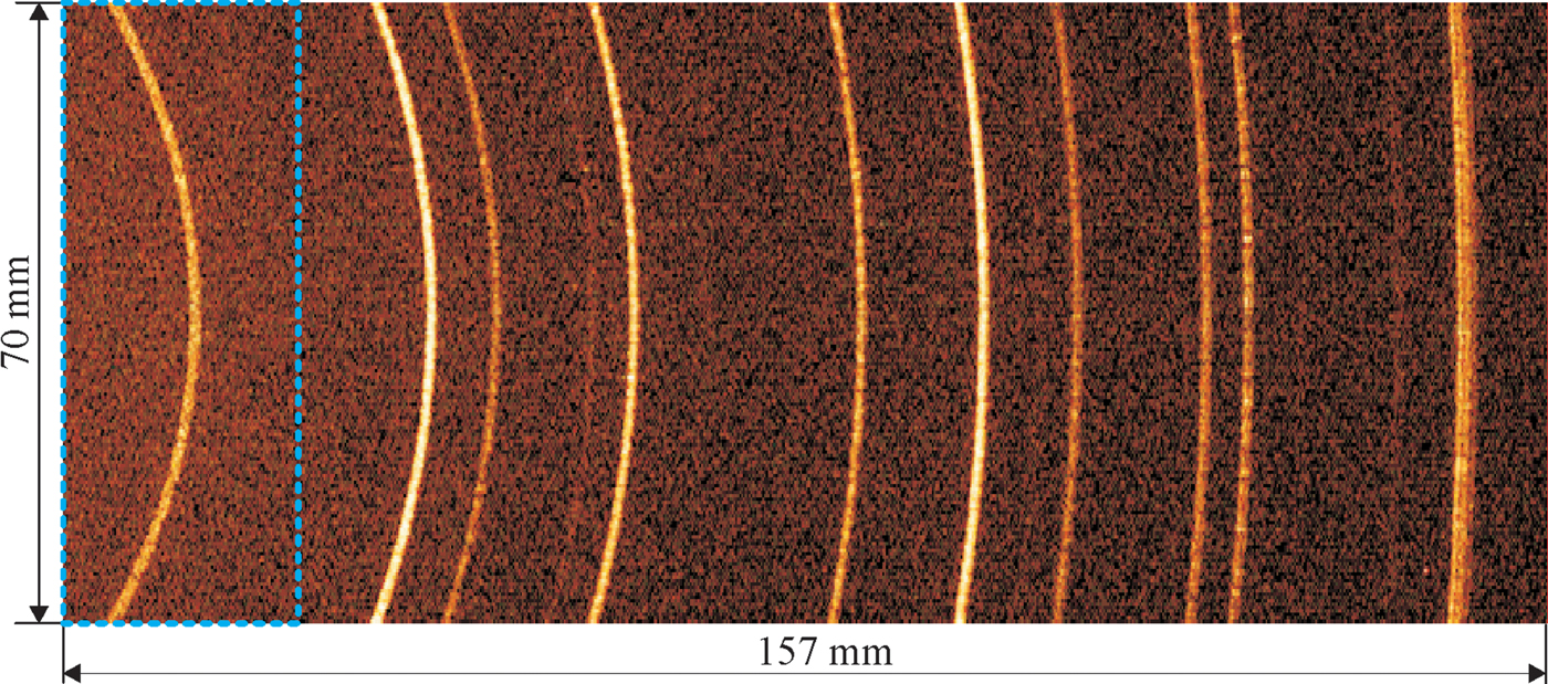
Figure 12. (Colour online) The 2D diffraction pattern collected from Corundum by scanning a rectangular 2D detector in γ-optimized mode within 2θ range of 20–80°.
VI. CONCLUSIONS
An XRD2 pattern covering a large angular range in both γ and 2θ can be collected by a 2D detector with the large active area. A large active area is a very important parameter in 2D detector selection, especially for applications requiring fast data collection, high-throughput screening or in situ measurement. When the 2θ coverage of the detector active area is not sufficient for the XRD2 applications, the 2θ coverage can be expanded by merging multiple frames or scanning 2D detector. The multiple frame merge method is suitable for the 2θ range covered by a few frames. The 2D detector scanning method is suitable to achieve a very large 2θ range, especially for smaller 2D detector or rectangular detector in γ-optimized mode. In order to achieve an accurate 2D diffraction pattern with expanded 2θ range, the frames collected by flat detectors are projected to a cylindrical surface for multiple frame merge or scanning image integration.