


I. INTRODUCTION
The use of a silicon strip X-ray detector (SSXD) has become quite popular in laboratory powder X-ray diffraction measurements. A typical SSXD consists of 128–256 PIN photodiodes, the width and length of which are 0.075–0.1 and 10–15 mm, respectively.
Figure 1 schematically illustrates the structure of an SSXD. The device is composed of densely P-doped Si strips, dilutely N-doped Si (intrinsic) layer, and densely N-doped Si layer. Reverse biased voltage applied to the device forms a depletion region in the intrinsic layer, and a photocurrent signal carried by an electron–hole pair generated by the absorption of an X-ray photon is detected through one of the P-doped strips, capacitively coupled to one of the integrated electronic circuits of amplifier, shaping and counting devices.

Figure 1. Schematic illustration of a silicon strip X-ray detector. The illustration is identical to that shown in a previous study (Ida, Reference Ida2020).
SSXD is particularly effective for the detection of CuKα (8 keV) X-ray, because the penetration depth of 8 keV X-ray into solid Si is estimated at μ −1 ≈ 0.07 mm, and it is expected that 99% photons are detected with 0.3 mm thickness of the intrinsic Si layer.
Mathematical formulas of the equatorial aberration function of a linear position-sensitive detector (LPSD) used in a step scan mode have been reported (Cheary and Coelho, Reference Cheary and Coelho1994; Słowik and Zięba, Reference Słowik and Zięba2001). Mendenhall et al. (Reference Mendenhall, Mullen and Cline2015) have proposed formulas of the numerical calculation of continuous-scan SSXD line profiles for a fundamental parameters approach model (Cheary and Coelho, Reference Cheary and Coelho1992). The author has compared the exact and the second-order (quadric) approximate formulas about the equatorial aberration of the continuous-scan SSXD data (Ida, Reference Ida2020), and suggested that the difference between the exact and approximate formulas might be detectable in a realistic configuration of a measurement system.
Manufacturers of laboratory powder X-ray diffractometers generally provide a continuous-scan integration (CSI) method of SSXD, where the incident glancing angle and the reflection glancing angle for the center strip of the SSXD are kept at the common angle. The X-ray photons counted by each of the off-centered detector strips at the offset angle of 2ψ are added to the counts for the nominal detector angle of 2Θ, when the incident glancing angle and the reflection glancing angle for the center strip are both Θ − ψ, as shown in Figure 2. The 2Θ diffraction is sensed 128 times by different detector strips on a single continuous scan with a 128-strip detector, and we can naturally expect that the sensitivity of the detection system is about 128 times higher than that available with a point detector, such as a scintillation counter.
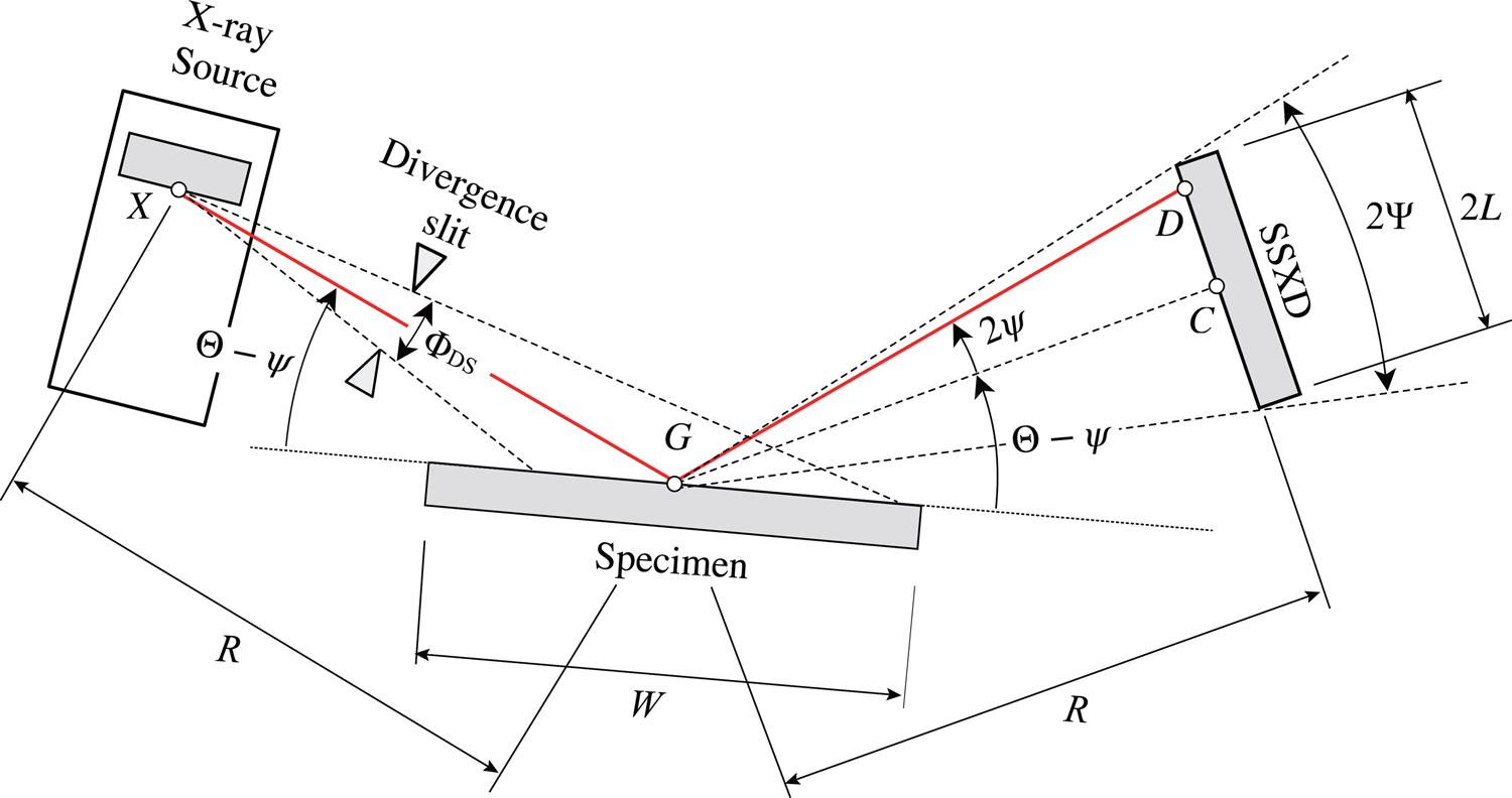
Figure 2. Instrumental parameters related to the continuous-scan integration of SSXD. The nomenclature is identical to that used in a previous study (Ida, Reference Ida2020).
The author would like to emphasize that the use of the CSI method is also effective for the improvement of particle statistics (de Wolff, Reference De Wolff1959) in powder diffractometry. The intensity allocated to the angle of 2Θ in the CSI-SSXD data is the integration of the diffraction intensities at the incident glancing angles from Θ − Ψ/2 to Θ + Ψ/2, when the view angle of SSXD is 2Ψ (see Figure 2). The probability that a randomly oriented crystallite can satisfy the diffraction condition and contribute to the observed diffraction intensity should become almost 100 times for the CSI data of a 128-strip detector, if the focal width of the X-ray source is similar to or narrower than the interval of the detector strips, as suggested by Yukino and Uno (Reference Yukino and Uno1986); Alexander et al. (Reference Alexander, Klug and Kummer1948) have shown that the effective particle dimension should be smaller than 10 μm, to achieve relative statistical error smaller than 1% in observed diffraction intensities from siliceous mineral powder in a typical powder X-ray diffraction measurement. The particle dimension may become about 50 μm, when the CSI of a 128-strip SSXD is applied.
II. THEORETICAL
A. Equatorial aberration of CSI of SSXD
The symbols for instrumental parameters related to the equatorial aberration of CSI-SSXD data are shown in Figure 2. R is the goniometer radius, W is the specimen width, and 2L is the effective length of SSXD. The deviation of the incident beam along the equatorial direction is primarily restricted by the divergence slit with the open angle of ΦDS, and the effective view angle of SSXD is denoted by 2Ψ.
Figure 3 illustrates the relations between the detector angle (nominal diffraction angle) 2Θ and the true diffraction angle 2θ, when the incident beam deviated by the angle of ϕ is reflected at the flat specimen face and detected by an off-center detector strip located at the offset angle of 2ψ. The deviation of the nominal diffraction angle from the true diffraction angle, Δ2Θ ≡ 2Θ − 2θ, is given by (Ida, Reference Ida2020)
 $$\Delta 2{\rm \Theta }( {{\rm \Theta }, \;\phi , \;\psi } ) = {\rm \Theta } + \phi + \psi -\arctan \displaystyle{{\sin ( {{\rm \Theta } + \psi } ) } \over {g( {{\rm \Theta }, \;\phi , \;\psi } ) }}, $$
 $$\eqalign{g( {{\rm \Theta }, \;\phi , \;\psi } ) &\equiv \cos ( {{\rm \Theta }-\psi } ) \cos 2\psi + \cos ( {{\rm \Theta } + \psi } ) \cr &\quad -\displaystyle{{\sin ( {{\rm \Theta }-\psi } ) \cos 2\psi } \over {\tan ( {{\rm \Theta }-\phi -\psi } ) }}.}$$
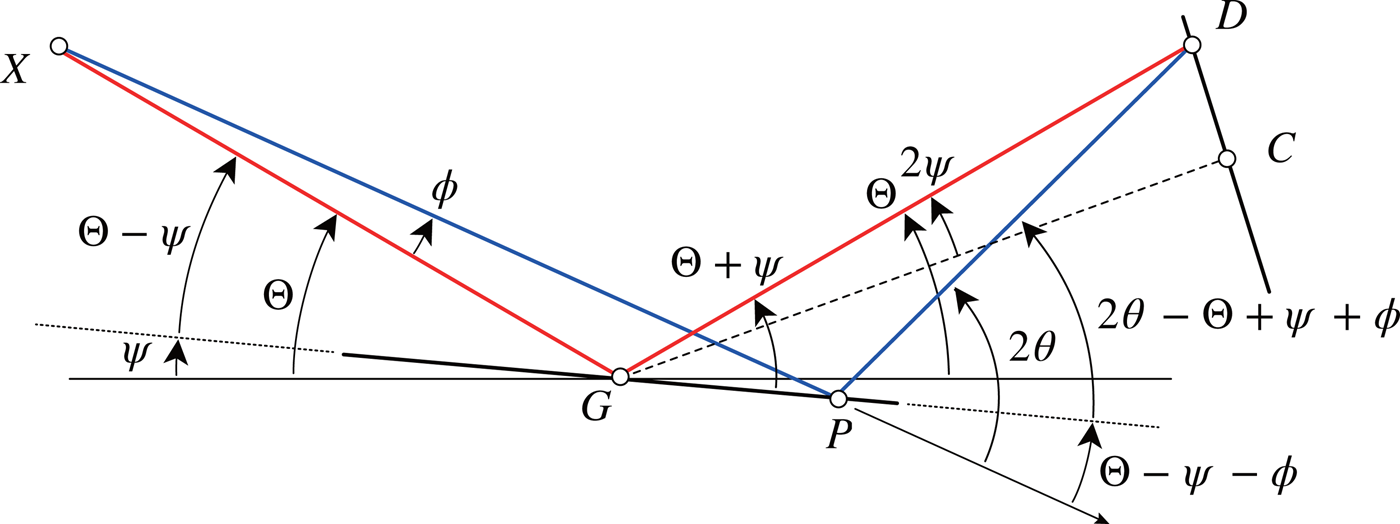
Figure 3. Relations between angles on continuous-scan integration of SSXD. The relations are identical to those shown in a previous study (Ida, Reference Ida2020).
The second-order expansion of Δ2Θ by ϕ and ψ straightforwardly gives an approximate formula,
 $$\Delta 2{\rm \Theta }( {{\rm \Theta }, \;\phi , \;\psi } ) \approx{-}\displaystyle{{2\phi ( {\phi + \psi } ) } \over {\tan {\rm \Theta }}}, $$
which is known as a kind of quadric surface, called a hyperbolic paraboloid.
When the incident glancing angle Θ − ψ (see Figure 2) is lower than the critical angle Θc, approximately given by
 $${\rm \Theta }_{\rm c}\approx \arcsin \displaystyle{{R{\rm \Phi }_{{\rm DS}}} \over W}, $$
for the divergence slit open angle of ΦDS, spillover of the irradiated area from the specimen face occurs.
In more detail, there should be four critical angles, Θc1, Θc2, Θc3, and Θc4, for the effects of spillover in the CSI-SSXD data, which are defined by the following equation,
 $$\tan \left({{\rm \Theta }_{{\rm c}j}-\psi \pm \displaystyle{{{\rm \Phi }_{{\rm DS}}} \over 2}} \right) = \displaystyle{{\sin ( {{\rm \Theta }_{{\rm c}j}-\psi } ) } \over {\cos ( {{\rm \Theta }_{{\rm c}j}-\psi } ) \mp W/2R}}, $$
for ψ = ±Ψ/2, when the center of the specimen face is perfectly located at the goniometer center. The solutions of Eq. (5) can numerically be evaluated by a bisection algorithm, for example. In case of  ${\rm \Phi }_{{\rm DS}} = 1.25^\circ$,
  $2{\rm \Psi } = 4.89^\circ$, R = 150 mm, and W = 20 mm, the values of the critical angles are estimated at
  $2{\rm \Theta }_{{\rm c}1} = 15.14^\circ$,
  $2{\rm \Theta }_{{\rm c}2} = 17.64^\circ$,
  $2{\rm \Theta }_{{\rm c}3} = 20.03^\circ$, and
  $2{\rm \Theta }_{{\rm c}4} = 22.53^\circ$, while the approximate value calculated by Eq. (4) is
  $2{\rm \Theta }_{\rm c} = 18.83^\circ$.
The lowest critical angle 2Θc1 corresponds to the solution for the deviation angle of ϕ = −ΦDS/2 and the offset angle of 2ψ = −Ψ, and the highest critical angle 2Θc4 corresponds to the solution for the deviation angle of ϕ = ΦDS/2 and the offset angle of 2ψ = Ψ. The effect of spillover is determined by the ratio W/R of the finite width of the specimen W and the goniometer radius R in the angular range 2Θ ≤ 2Θc1, while it is determined by the divergence slit open angle ΦDS in the range 2Θc4 ≤ 2Θ of the CSI-SSXD data. It should be noted that the effects of spillover are dependent on the offset angle 2ψ of a detector strip, in a finite data range 2Θc1 < 2Θ < 2Θc4, which can hardly be neglected.
The author suggest that the implementation of treatments on such complicated geometrical relations about the CSI-SSXD data would be more straightforwardly and safely achieved by keeping the exact mathematical expressions rather than looking for any approximation.
The effective lower and upper limits, Φ0(ψ) and Φ1(ψ) of the equatorial deviation angle ϕ, diffracted by the specimen and detected by the strip at the offset angle 2ψ are generally given by
 $${\rm \Phi }_0( \psi ) = {\rm max}\left\{{-\displaystyle{{{\rm \Phi }_{{\rm DS}}} \over 2}, \; {\rm \Theta }-\psi -\arctan \displaystyle{{\sin ( {{\rm \Theta }-\psi } ) } \over {\cos ( {{\rm \Theta }-\psi } ) -W/2R}}} \right\}, $$
 $${\rm \Phi }_1( \psi ) = {\rm min}\left\{{\displaystyle{{{\rm \Phi }_{{\rm DS}}} \over 2}, \;{\rm \Theta }-\psi -\arctan \displaystyle{{\sin ( {{\rm \Theta }-\psi } ) } \over {\cos ( {{\rm \Theta }-\psi } ) + W/2R}}} \right\}.$$
The first to fourth-order cumulants of the exact equatorial aberration function, κ 1, κ 2, κ 3, and κ 4 are numerically calculated by applying the following equations,
 $$\kappa _1 = \displaystyle{{s_1} \over {s_0}}, $$
 $$\kappa _2 = \displaystyle{{s_2} \over {s_0}}-\displaystyle{{s_1^2 } \over {s_0^2 }}, $$
 $$\kappa _3 = \displaystyle{{s_3} \over {s_0}}-\displaystyle{{3s_2s_1} \over {s_0^2 }} + \displaystyle{{2s_1^3 } \over {s_0^3 }}, $$
 $$\kappa _4 = \displaystyle{{s_4} \over {s_0}}\;-\displaystyle{{4s_3s_1} \over {s_0^2 }}-\displaystyle{{3s_2^2 } \over {s_0^2 }} + \displaystyle{{12s_2s_1^2 } \over {s_0^3 }}-\displaystyle{{6s_1^4 } \over {s_0^4 }}, $$
 $$\eqalign{s_k =& {\rm \Psi }\mathop \sum \limits_{i = 1}^N w_i[ {{\rm \Phi }_1( {\psi_i} ) -{\rm \Phi }_0( {\psi_i} ) } ] g_\psi ( {\psi_i} ) \cr & \times \mathop \sum \limits_{\,j = 1}^N w_j[ {\Delta 2{\rm \Theta }( {\phi_{ij}, \psi_i} ) } ] ^kg_\phi ( {\phi_{ij}} ),}$$
 $$\phi _{ij} = {\rm \Phi }_0( {\psi_i} ) + x_j[ {{\rm \Phi }_1( {\psi_i} ) -{\rm \Phi }_0( {\psi_i} ) } ] , $$
 $$\psi _i = {-}\displaystyle{{\rm \Psi } \over 2} + x_i{\rm \Psi }, $$
where {x i} are the relative locations and {w i} are the weights for sampling points on numerical integral, and  $g_\phi ( \phi )$ and
  $g_\psi ( \psi )$ are the density functions of the distribution of the intensity of the incident beam for deviation angle ϕ and the sensitivity of the detector at the offset angle ψ, respectively.
The uniform distributions,  $g_\phi ( \phi ) = 1/{\rm \Phi }_{{\rm DS}}$ and
  $g_\psi ( \psi ) = 1/{\rm \Psi }$, are assumed here, but it is not difficult to incorporate any distribution or noncylindrical correction for a flat detector, for example, in the current algorithm. It is expected that the use of an approximate aberration model function based on the uniform distribution should still be effective, when the realistic intensity/sensitivity distribution is not far from the uniform distribution, as will be discussed later.
The values s 0 calculated by Eq. (12) for all the 2Θ values are identical to unity in the 2Θ region 2Θc4 ≤ 2Θ, where spillover does not occur, while they correspond to the relative intensities reduced by the spillover effect for the lower 2Θ angles, 2Θ < 2Θc4. The reduction of the intensities is corrected just by the division of the intensity data by the values s 0.
Since the main feature of the relation given by Eqs (1) and (2) is well reproduced by the quadric formula given by Eq. (3) (Ida, Reference Ida2020), it is expected that the Gauss–Legendre quadrature should be effective on numerical integration expressed by Eqs (12)–(14) (Press et al., Reference Press, Teukolsky, Vetterling and Flannery2007).
It has been found that the numerical evaluation by 4 × 4 point Gauss–Legendre quadrature for the third-order cumulant of Δ2Θ for the values  $2{\rm \Theta } = 30^\circ$,
  ${\rm \Phi } = 1.25^\circ$, and
  $2{\rm \Psi } = 4.89^\circ$ certainly gives similar accuracy to the value evaluated by 1000 × 1000 mid-point method applied in a previous study (Ida, Reference Ida2020). The numerical values of locations {x i} and weights {w i} for four-point Gauss–Legendre quadrature are listed in Table I.
TABLE I. Relative locations {x i} and weights {w i} of four-point Gauss–Legendre quadrature.

B. Naïve two-step deconvolutional method to remove the effects of first and third-order cumulants of an aberration function
The author has proposed a method to multiply the complex absolute value of the Fourier transform of the instrumental function, on the division of the Fourier transform of the observed data by the Fourier transform of the instrumental function, on the Fourier-based deconvolution process (Ida et al., Reference Ida, Ono, Hattan, Yoshida, Takatsu and Nomura2018).
It is assumed that the first and third-order cumulants of the instrumental aberration function ω(Δ2Θ; 2Θ) are dependent on the detector angle 2Θ and given by functions κ 1(2Θ) and κ 3(2Θ), respectively. It is also assumed that the first and third-order cumulants of a function w(x) are given by constant values, k 1 and k 3. The first-order cumulant of the function shifted by −k 1, w(x + k 1), should be zero, and the third-order cumulant of the function w(x + k 1) should still be k 3.
At the first step of a naïve two-step deconvolutional method, the scale transform from 2Θ to χ 3, given by
 $$\chi _3( {2{\rm \Theta }} ) = k_3^{1/3} \int {\displaystyle{{\;{\rm d}2{\rm \Theta }} \over {\kappa _3^{1/3} ( {2{\rm \Theta }} ) }}} $$
is used, and the deconvolutional treatment about the function w(χ 3 + k 1) is applied on the χ 3 scale. After the treatment, the effect of the third-order cumulant of the aberration function κ 3(2Θ) is removed, while the effect of the first-order cumulant should not be changed from κ 1(2Θ) on the 2Θ scale.
The first-order cumulant of the Dirac delta function shifted by k 1, δ(x − k 1), is k 1, and all the cumulants of the function δ(x − k 1) of the order higher than the first are zero. At the second step of the naïve two-step deconvolutional method, another scale transform from 2Θ to χ 1, given by
 $$\chi _1( {2{\rm \Theta }} ) = k_1\int {\displaystyle{{\;{\rm d}2{\rm \Theta }} \over {\kappa _1( {2{\rm \Theta }} ) }}} $$
is used, and the deconvolutional treatment about the function δ(χ 1 − k 1) is applied on the χ 1 scale. After the second treatment, the effects of both the first and third-order cumulants κ 1(2Θ) and κ 3(2Θ) should exactly be removed from the experimental data on the 2Θ scale.
The integrals of Eqs (15) and (16) are recurrently evaluated in the numerical calculation, by applying the following equations,
 $$\chi _k( {2{\rm \Theta }_0} ) = 0, $$
 $$\chi _k( {2{\rm \Theta }_j} ) = \chi _k( {2{\rm \Theta }_{j-1}} ) + {\rm \;}\displaystyle{{k_k^{1/k} \;( {2{\rm \Theta }_j-2{\rm \Theta }_{j-1}} ) } \over {\kappa _k^{1/k} ( {2{\rm \Theta }_j} ) }}.$$
If the model function w(x) is identical to the aberration function ω(Δ2Θ; 2Θ) on an appropriately transformed scale, this naïve two-step method is equivalent to a one-step deconvolutional method, where the effects of all the odd-order cumulants of the aberration function should be removed, which may be called as symmetrization (Ida and Hibino, Reference Ida and Hibino2006). On the other hand, the naïve two-step method can remove the effects of the first and third-order cumulants, even if the model function w(x) is not identical to the aberration function ω(Δ2Θ; 2Θ) on any transformed scales.
This naïve two-step method never appears ideal to the author, while more sophisticated formulation of a two-step method has already been proposed for treatment of the axial-divergence aberration (Ida et al., Reference Ida, Ono, Hattan, Yoshida, Takatsu and Nomura2018). However, it is expected that the naïve method is still effective for treatment of the equatorial aberration in the data collected by CSI of SSXD, partly because an explicit expression of the quadric approximate model function in the non-spillover region (Ida, Reference Ida2020) can be used, and it is expected that the introduction of the numerically evaluated exact values of the cumulants will improve the approximation, not only for the data affected by the spillover, but also for the data in the non-spillover region.
C. Model aberration profile function
A model aberration profile function w(χ) is derived by the application of an analytical formula for the scale transform from 2Θ to χ, given by
 $$\chi ( {2{\rm \Theta }} ) = \displaystyle{{12\ln \sec {\rm \Theta }} \over {{\rm \Phi }_{{\rm DS}}^2 }},$$
to an explicit quadric expression of the aberration function (Ida, Reference Ida2020). Note that the effects of kth order cumulants of the approximate aberration function ω(Δ2Θ; 2Θ), the scale parameter of which is proportional to  $\cot ^k{\rm \Theta }$, can be considered as a convolution on the χ scale defined by Eq. (19), because the differential of Eq. (19) by 2Θ gives
 $$\displaystyle{{{\rm \Delta }\chi } \over {{\rm \Delta }2{\rm \Theta }}} = \displaystyle{{6\tan {\rm \Theta }} \over {{\rm \Phi }_{{\rm DS}}^2 }}\;.$$
The normalized expression of the function w(χ) for ρ ≡ Ψ/ΦDS is given by
 $$w( \chi ) = \left\{{\matrix{ {\displaystyle{1 \over {6\rho }}\ln \displaystyle{{\phi_{\rm U}} \over {\phi_{\rm L}}}}, & {[ {\chi_{{\rm min}} < \chi < \chi_{{\rm max}}} ] }, \cr 0, & {[ {{\rm elsewhere}} ] }, } } \right.$$
 $$\chi _{{\rm min}} = {-}3( {1 + \rho } ) ,$$
 $$\chi _{{\rm max}} = \left\{{\matrix{ {-3( {1-\rho } ) }, & {[ {2 < \rho } ] }, \cr {\displaystyle{{3\rho^2} \over 4}}, & {[ {\rho \le 2} ] },} } \right.$$
 $$\phi _L = {\rm max}\left\{{-\rho + \sqrt D , \;\rho -\sqrt D \;} \right\}, $$
 $$\phi _U = {\rm min}\left\{{2, \;\rho + \sqrt D } \right\},$$
 $$D = \rho ^2-\displaystyle{{4\chi } \over 3}.$$
The first to fourth-order cumulants of the function w(χ), k 1, k 2, k 3, and k 4, are given by
 $$k_1 = {-}1, $$
 $$k_2 = \displaystyle{4 \over 5} + \rho ^2, $$
 $$k_3 = {-}\displaystyle{{16} \over {35}}\left({1 + \displaystyle{{21\rho^2} \over 4}} \right), $$
 $$k_4 = {-}\displaystyle{{96} \over {175}}\left({1-5\rho^2-\displaystyle{{7\rho^4} \over {16}}} \right).$$
III. EXPERIMENTAL
Three powder specimens of LaB6 (NIST SRM660c) with the widths of W = 20, 10, and 5 mm along the equatorial direction have been prepared to test the performance of the current algorithm against the spillover effects on the equatorial aberration.
A desktop powder diffractometer (Rigaku, MiniFlex 600-C, R = 150 mm) with an SSXD (Rigaku, D/teX Ultra-2, 128 strips with 0.1 mm interval) and a measurement/control software SmartLab Studio II were used to collect powder diffraction data. The view angle of the SSXD is estimated at  $2{\rm \Psi } = 4.89^\circ$. A copper-target X-ray tube (Canon Electron Tubes & Devices, A-21-Cu, effective focal size of 0.1 mm × 10 mm) was operated at 40 kV and 15 mA. A divergence slit with the open angle of
  ${\rm \Phi }_{{\rm DS}} = 1.25^\circ$, a couple of Soller slits with the nominal open angle of
  $1.25^\circ$, and a nickel foil filter with the thickness of 0.032 mm to reduce CuKβ X-rays were used.
The 2Θ range from  $5^\circ$ to
  $140^\circ$ was continuously scanned at the scan rate of
  $0.4^\circ {\rm min}^{-1}$, and the intensity data were collected at the 2Θ step interval of
  $0.01^\circ$. Total measurement time was about 350 min for each scan.
The highest critical angle 2Θc4, where the effects of the spillover of the incident beam should appear, is estimated at  $2{\rm \Theta }_{{\rm c}4} = 22.5^\circ , \;\;41.9^\circ$, and
  $85.5^\circ$ for the specimen widths of W = 20, 10, and 5 mm, respectively, while the LaB6 100 peak is located at
  $2\theta _{100} = 21.36^\circ$.
IV. RESULTS
The observed powder diffraction intensity data from three LaB6 specimens, with the widths of W = 20, 10, and 5 mm, are shown in Figure 4. The four critical angles related to the effects of the spillover for each of the specimens are indicated by vertical broken lines in Figure 4. It should be better to know the values of the four critical angles, whenever a CSI-SSXD method is used, even if it may appear unnecessary to the users of the current algorithm.

Figure 4. Diffraction intensities observed for LaB6 specimens with the widths of W = 20, 10, and 5 mm. Vertical broken lines indicate four critical angles about the effects of spillover for each specimen.
The results of the deconvolutional treatments (DCTs) to the observed data are shown in Figure 5. Treatments about the spectroscopic profile of the source X-ray, axial divergence, and sample transparency aberrations have been applied, in a manner similar to the previous study (Ida, Reference Ida2020). The effects of spillover on the intensities and deformation of the peaks through the equatorial aberration are automatically treated with the current version of a software implemented by Python 3.7.6 with SciPy 1.3.1 library, just by indicating the values of the goniometer radius R = 150 mm, specimen width W = 20, 10, or 5 mm, divergence slit angle  ${\rm \Phi }_{{\rm DS}} = 1.25^\circ$, and the view angle of SSXD
  $2{\rm \Psi } = 4.89^\circ , \;$ in a configuration file for the program. The computing time was about 3 s for the treatment of one diffraction pattern on a Python interpreter system running on a laptop computer (Apple, macOS 10.15.5, MacBook Pro with 2.8 GHz quad-core Intel i7 processor).

Figure 5. Results of deconvolutional treatments to the observed data shown in Figure 4.
The results of the DCTs on the collected data are shown in Figure 5. The most significant change in the profiles of the data sets before and after the treatments (Figures 4 and 5) should be the disappearance or reduction of the CuKα 2 peaks. The r eduction of small CuKβ peaks and step structures caused by the Ni K absorption edge in the background intensities are also detectable. All the parameters about the spectroscopic profile of the source X-ray are the same as those used in a previous study (Ida, Reference Ida2020).
The LaB6 100-diffraction peak profiles in the observed (Figure 4) and the deconvolutionally treated (Figure 5) data sets from the specimens with the widths of W = 20, 10, and 5 mm are shown in Figure 6. Note that the profile of the widest specimen W = 20 mm [Figure 6(a)], the dimension of which is usually available for powder diffraction users, should slightly be affected by the spillover of the incident X-ray beam under the current measurement condition, because the data are collected by a CSI-SSXD method.

Figure 6. The LaB6 100-diffraction peak profiles in the observed (solid circles) and deconvolutionally treated (open circles) data sets for the specimen widths of (a) W = 20 mm, (b) W = 10 mm, and (c) W = 5 mm. Symmetric Voigtian curves fitted to the DCT data are drawn as solid lines.
The observed LaB6 100-diffraction peak profiles in Figure 6 show a tendency, which implies that a narrower specimen gives weaker intensities but a sharper profile. The 2:1-doublet profile of CuKα 1 and CuKα 2 electronic structure (separated by spin-orbit coupling) is detectable in the profile shown in Figure 6(c), but it would be difficult to find that the same structure is commonly included in the observed peak profiles shown in Figures 6(b) and 6(a).
The peak profiles in the results of the DCTs on the CSI-SSXD data in Figure 6 appear more symmetric than those of the observed data, as expected. The curves fitted to the DCT data by a Voigt function model do not show any severe discrepancy in the current algorithm.
One may think that the deconvolutional treatment on powder diffraction data collected by a CSI-SSXD method would be useful for identification of materials, crystal structure refinements, precise evaluation of lattice constants, microstructure analysis including crystallite size evaluation, and so on. All the Python codes used in this study are freely available from a website of the author.
V. CONCLUSION
A deconvolutional method to treat powder diffraction data collected by CSI-SSXD has been formulated and implemented by Python with SciPy library. Reduction of intensities caused by the effects of spillover of the incident X-ray beam from the specimen face at lower diffraction angles is automatically corrected in the current algorithm. Exact values of cumulants of the equatorial aberration function are efficiently evaluated by 4 × 4 point two-dimensional Gauss–Legendre integral.
A naïve two-step deconvolutional treatment has been applied to remove the effects of the first and third-order cumulants of the equatorial aberration function from the observed CSI-SSXD data. The algorithm has been tested by the analyses of CSI-SSXD data of three LaB6 powder specimens with the widths of 20, 10, and 5 mm. No significant discrepancy has been found in the treated data, where it is expected that the intensity reduction, peak shift, and asymmetric deformation of the peak profile should be corrected by the treatment.
ACKNOWLEDGEMENTS
The experimental part of this study has been financially supported by JSPS KAKENHI Grant No. 19H02747, which allowed the author to use a desktop XRD measurement system with a silicon strip X-ray detector.


