II. EXPERIMENTAL

To perform the XRD/XRF mappings, an INEL Equinox 3500 combined instrument equipped with a single X-ray source with two detectors for XRD and XRF operating simultaneously was adopted (Lutterotti et al., Reference Lutterotti, Dell'Amore, Angelucci, Carrer and Gialanella2016) (Bortolotti et al., Reference Bortolotti, Lutterotti and Pepponi2017) (Figure 1).

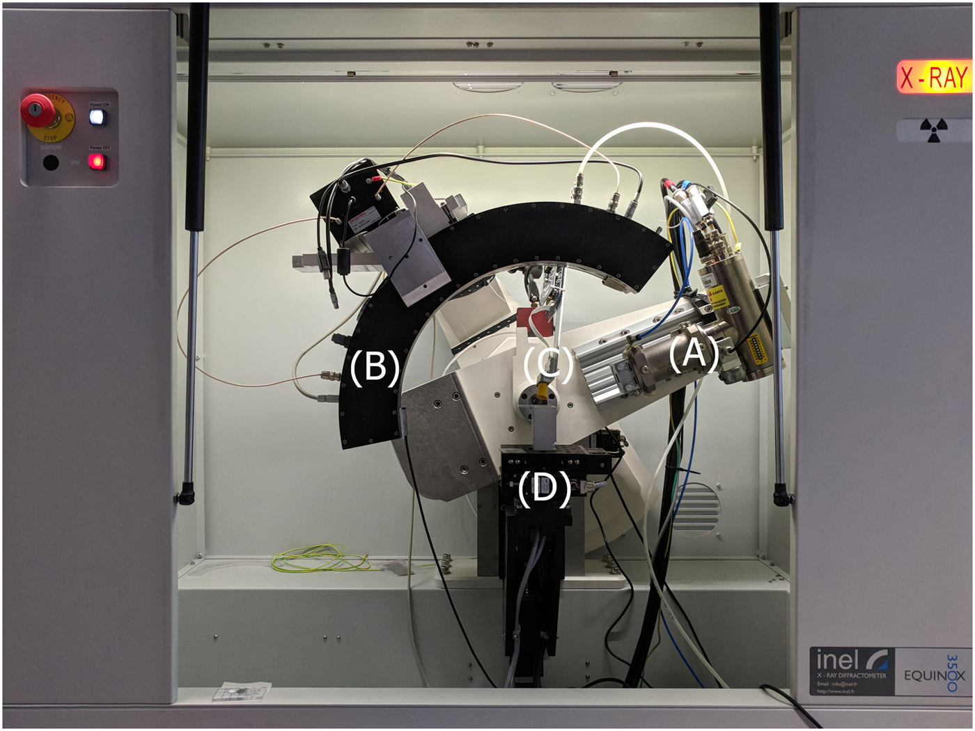
Figure 1. The combined XRD/XRF instrument for automated 2D data collection. (a) Microfocus Mo source (b) CPS120 XRD Curved Position Detector (c) Si Pin XRF detector (d) XYZ motorized sample stage.

The machine was equipped with a 50W microfocus source with Mo target (Figure 1(a)) coupled with a multilayer elliptic mirror (AXO Dresden GmbH) to suppress k-β radiation and provide a quasi-parallel beam; the single source setup ensures that both XRD and XRF signals are recorded from exactly the same point on the surface. Beam size on the sample was reduced by means of manual cross-slits to about 1 × 0.5 mm². A curved position sensitive detector (Figure 1(b)) was used to collect diffraction data (INEL CPS120); the detector operated over 120° in 2 θ with a 4096 channel resolution. Fluorescence spectra were collected by means of a Si-PIN diode (Figure 1(c)) coupled to a 4096 channel analyzer (Moxtek X-PIN50). Finally, a 3-axis motorized sample holder (Oriental Motors) was used to automate the x–y mappings with a scan step resolution of 0.5 mm (Figure 1(d)).

Both XRD and XRF detector operated in a fixed position to ensure the fastest data collection possible; acquisition times of 60 s were chosen as a compromise between data collection speed and signal quality.

For the validation of the different clustering strategies and their relative performances, synthetic samples were prepared with ad-hoc designed chemical and crystallographic surface features. The first sample (Figure 2(a)) was prepared by embedding a steel alloy cube (6 mm edge) in a metallographic resin, with the goal to provide the simplest classification problem possible (two classes). The second sample (Figure 2(b)) was designed to offer a more challenging benchmark for assessing classification performance: five different metallic rods based on different alloy compositions (Brass, Copper, Aluminium, Titanium) with diameters ranging from 3 to 7 mm were embedded in an amorphous metallographic resin. Both samples were cut and polished to obtain an ideally flat surface for the data collection.

Figure 2. Synthetic samples providing a test suite for evaluating the performance of the different data clustering strategies. (a) Steel alloy cube embedded in resin; (b) metallic rods embedded in amorphous resin.

III. ANALYTICAL METHODOLOGY

Data clustering is one of the many available tools among data mining methodologies, whose main goal consists in finding subgroups (clusters) of similar observations inside a data set. Data clustering can be implemented by a large variety of algorithms (Kaufman et al., Reference Kaufman, Kaufman, Rousseeuw and Rousseeuw2005), (Tan et al., Reference Tan, Steinbach and Kumar2005); for the aim of this work, three different clustering algorithms have been selected among the most widely adopted in various application fields, namely hierarchical clustering (HC), k-means clustering (KM), and density-based clustering (DB).

The classification process is not an automatic task: clustering parameters (dissimilarity metric, number of expected clusters, minimum observations number to define a cluster, etc.) depend on both the algorithm chosen and, of course, on the data domain under consideration; indeed, it is often the case, that the best clustering algorithm as well as its operating parameters need to be chosen experimentally for a specific problem solving. In particular, the choice of the dissimilarity criterion is often critical as it defines how two observations in a data set can be considered distant from each other in the data set space. Several distance metrics have been defined for different application domains; some commonly used metrics in cluster analysis are Euclidean distance, squared Euclidean distance and Manhattan distance, as defined below:

(1)$$d(i,j)_{{\rm euclidean}} = \sqrt {\sum\limits_m {{(i_m-j_m)}^2}} $$

(2)$$ \!\!\!\!\!\!\!d(i,j)_{{\rm euclidea}{\rm n}^{\rm 2}} = \sum\limits_m {{(i_m-j_m)}^2} $$

(3)$$\!\!\!\!\!\!\!\!\!\!d(i,j)_{{\rm manhattan}} = \sum\limits_m {\vert {i_m-j_m} \vert } $$

In our case, the standard Euclidean distance was chosen as the default metric for all the clustering algorithms, as it turned out to be the best performing in all cases.

In the following, we briefly describe the basic operation of the different clustering algorithms.

HC (Lance and Williams, Reference Lance and Williams1967) classifies objects by performing a subdivision of the data set into a hierarchy of different subgroups based on their relative distances; classification can proceed in an agglomerative fashion (all observations start as distinct clusters, which are then merged based on their similarity) or a divisive one (all the observations starts inside a single cluster, which is then subdivided in successive iterations). In addition to the distance between each observation, another important decision needed by HC is the linkage criterion between clusters, that is the criterion by which two clusters C _i and C _j are classified based on the pairwise distances between the n _i, n _j observations they contain. Some commonly used strategies are single linkage, based on the minimum distance found between observations in the two clusters (eq. (4)), complete linkage, based on the maximum distance (eq. (5)), and average linkage, defined as the average distance between each point in one cluster to every point in the other cluster (eq. (6)); this latter criterion is also the one adopted in the current work.

(4)$$\max {\mkern 1mu} \{ {\mkern 1mu} d(i,j):i\in C_i,{\mkern 1mu} j\in C_j{\mkern 1mu} \} $$

(5)$$\min {\mkern 1mu} \{ {\mkern 1mu} d(i,j):i\in C_i,{\mkern 1mu} j\in C_j{\mkern 1mu} \} $$

(6)$$\displaystyle{1 \over { \vert C_i \vert \vert C_j \vert}} \mathop \sum \limits_{i\in C_i} \mathop \sum \limits_{\,j\in C_j} d(i,j)$$

HC does not provide a unique partitioning of the data set; the principal output of the algorithm is a dendrogram, a hierarchical plot, where the y-axis represents the distance at which different clusters merge; the user still needs to decide at which distance to cut the tree, obtaining a partitioning at a selected precision and a corresponding number of clusters.

The standard algorithm has a time complexity of ${\cal O}(n^3)$ and is thus not suitable for highly complex problems; for the scope of the current work, this is a negligible shortcoming but could become problematic for large data sets.

KM clustering (Macqueen, Reference Macqueen1967) is a kind of centroid-based clustering algorithm in which cluster centers are represented by a vector in the data set p-space; center points can belong to the cluster itself or not. The original algorithm was originally designed for signal processing (Lloyd, Reference Lloyd1982) and aims to partition an n-point data set into k cluster centers (with k < n), grouping the n observations in the different clusters in such a way to minimize the within-cluster sum of squared distances:

(7)$$\mathop {{\rm min}}\limits_C \sum\limits_{i = 1}^k {\sum\limits_{{\vector x}\in C_i} {{\left\ \vert {x-{\rm \mu} _i} \right\ \vert} ^2}} $$

where μ _i is the center of cluster C _i (e.g. the mean of points contained in cluster C _i) and both x and μ _i are p-dimensional vectors. The general solution to the problem is NP-hard; when the number of clusters k and the dimensionality of the space p are fixed in advance, the time complexity can be reduced to O(n ^pk+1), still computationally significant for all but the most trivial applications. Thus, only approximate solutions (local optima) can be found, by using for example the Lloyd's heuristic algorithm (Lloyd, Reference Lloyd1982), also adopted in this work; in cases like this, it is common practice to run the iteration several times and pick the best solution found among the different runs.

The main disadvantage of the algorithm is that it requires the knowledge of the number of clusters in advance; also, KM clustering tends to prefer clusters of the same size (since it is based on the distance from the centroid), often producing incorrectly cut cluster borders.

A final clustering strategy examined was DB clustering. DB clustering is based on the distinction between high-density areas in the data set, which can be classified as actual clusters, and low-density areas which are treated as noise or cluster borders. The most famous algorithm for performing DB clustering is DBSCAN (Ester et al., Reference Ester, Kriegel, Sander and Xu1996), which works by grouping points within certain distance thresholds. The main advantage of this algorithm is that, differently from HC and KM, it can find arbitrarily shaped clusters in the p-space; additionally, the number of clusters is not required as an input, and it is quasi-deterministic (core points classification is deterministic whereas border points classification can sometimes be non-deterministic). DBSCAN has a fast average converging time of O(nlog n). As the negative features, this algorithm assumes clusters of similar densities and requires an additional range parameter as input. An extension of the method, OPTICS, which does not suffer from these issues was recently proposed (Ankerst et al., Reference Ankerst, Breunig, Kriegel and Sander1999) and has been adopted in this work as a reference implementation for DB methods.

Relative performances of different clustering methods on the same data set can be evaluated with several numerical criteria (Theodoridis and Koutroumbas, Reference Theodoridis and Koutroumbas2009), which can be broadly distinguished into two main strategies: internal and external evaluation. Internal evaluation is based on the same data used for clustering; in general, the quality scores are biased towards high intra-cluster and low inter-clusters similarity. As such, internal evaluation criteria can suggest how different algorithms perform but not necessarily the quality of the clustering itself. One of the most used internal validation criteria is the Dunn index (Dunn, Reference Dunn1974):

(8)$${\rm DUNN} = \displaystyle{{\mathop {\min} \limits_{1 \le i \lt j \le n} d(i,j)} \over {\mathop {\max} \limits_{1 \le k \le n} {d}^{\prime}(k)}}{\mkern 1mu} $$

where d(i, j) represents the value of the adopted distance metric calculated between clusters i and j, whereas d’(k) measures the intra-cluster distance of cluster k.

In the external evaluation, clustering performances are compared against some reference benchmark of pre-classified data. A large selection of numerical criteria can be found in the literature; in this work we have chosen the widely adopted Rand index (Rand, Reference Rand1971), which is a measure of the similarity between the trial clustering classification and the benchmark:

(9)$${\rm RAND} = \displaystyle{{{\rm TP} + {\rm TN}} \over {{\rm TP} + {\rm FP} + {\rm FN} + {\rm TN}}}$$

where TP is the number of true positives, TN is the number of true negatives, FP is the number of false positives, and FN is the number of false negatives. It is also possible to define a chance-corrected adjusted Rand index (Rand, Reference Rand1971), which takes into account the weight difference between false positives and false negatives. In both cases, the Rand index may take values from −1 (meaning the classifications are completely uncorrelated) to 1 (perfect correlation).

In the present work, the clustering evaluation procedure begins starting from the calculation of the Euclidean distance matrix of the XRD and XRF data sets. Each matrix is n × n dimension, where n is the total number of experimental data points, which are typically (but not necessarily) collected over a square k × k points grid. Each matrix element d _ij corresponds to the Euclidean distance between i and j points; the matrix is thus symmetric and the diagonal elements are equal to one. Each observation is associated with p features, which in our case are represented by distinct measurements of integrated X-ray counts collected over a discrete interval (Bragg angle or Energy). Additionally, the combined distance matrix is calculated, with each element d _comb,ij equal to the sum of the XRD and XRF Euclidean distances:

(10)$$d_{{\rm comb},ij} = \sqrt {d_{{\rm xrd,}ij}^2 + d_{{\rm xrf,}ij}^2} $$

Clustering algorithms are then executed on the different distance matrices, and their results numerically compared by the means of adjusted Rand index; finally, a contour map of the sample surface is reconstructed based on the cluster assignment of each measurement point.

All calculations of this work have been performed using the package R (R Development Core Team, 2016), with the aim of the additional packages “Cluster” (Maechler et al., Reference Maechler, Struyf, Hubert, Hornik, Studer and Roudier2015), “Factoextra” (Kassambara and Mundt, Reference Kassambara and Mundt2017) and “DBSCAN” (Hahsler and Piekenbrock, Reference Hahsler and Piekenbrock2017) for cluster analysis; a source code example for testing the methodologies described is provided in the online supplementary material.

IV. RESULTS AND DISCUSSION

We report here qualitative and quantitative results obtained from cluster classification applied to the samples described in the experimental section.

Sample 1 was used as a simple test case to perform a preliminary evaluation of the relative strengths and weaknesses of different clustering strategies. Given the sample basic geometry, a coarser mapping was performed using only a 21 × 21 point matrix over a 12 × 12 mm² area; Figure 4(a) reports the ideal cluster classification as obtained from the optical image color discretization of the area under consideration. As reported in Table I, all of the clustering algorithms offered good classification performance on the XRF data set, with values of the Corrected Rand index above 0.8; on the other hand, bot HC and KM provided poor performance on the XRD data set, with DB clustering completely failing. When using the combined distance matrix to perform the classification, both HC and KM algorithms were able to improve the performance with respect to the single XRD and XRF data set; DB was able to correctly perform the classification, albeit with a lower Rand value with respect to the XRF data alone. As an example, we also report here qualitative results obtained from HC clustering on the XRD data set. In Figure 3(a), the dendrogram plot of the Euclidean distance matrix calculated on the XRD data is represented; the partitioning shows tree principal clusters, corresponding to the steel sample, the matrix and a “noise” cluster of unidentified points. Figure 3(b) reports the corresponding cluster plot representing the grouping of each data point in the data set, after the dendrogram cut performed at a number of clusters equal to 3.

Figure 3. (a) Dendrogram plot obtained from the hierarchical clustering classification on the XRD data set; (b) cluster plot on the same data after the dendrogram cut corresponding to three clusters.

Figure 4. Sample 1 area reconstruction based on the Hierarchical Clustering classification performed on the distance matrix calculated on the XRD data set (b), XRF data set (c) and combined data set (d). (a) represents the reference classification obtained from the color discretization of the optical image of the area under consideration.

TABLE I. Corrected Rand index values obtained from the comparison between the data clustering runs performed on sample 1 and sample 2 and their relative reference classifications.

Figure 4 reports the area reconstructions of the sample surface based on the different classifications. Figure 4(a) shows the ideal classification, as obtained from the optical image of the sample; Figures 4(b) and (c) show the reconstruction performed starting from the XRD and XRF data sets, respectively, evidencing the poor performance of the XRD data set as compared to the XRF one. Finally, the combined data set shows a slight improvement in the sample/matrix interface reconstruction with respect to the XRF case (Figure 4(d)).

The second sample was used as a test to provide more realistic quantitative performance results from the different classification algorithms. The same algorithmic strategy was chosen, testing three different clustering algorithms on the Euclidean distance matrix calculated from the single data sets as well as the one obtained from the sum of the distances, for a total of nine classification runs. In this case, the corrected Rand index values are in general much lower (Table I), meaning a lower general agreement between the reference classification, and the one obtained from the clustering. For this test sample, classification performed on XRD data set alone performed better than on the XRF data set, with the exception of the DB strategy which failed. Classification performed on the combined distance matrix, on the other hand, gave slightly improved results compared to the XRD data set in the case of KM and HC; the DB algorithm was able to run correctly but gave a Rand Index of almost zero (no correlation).

Examination of the reconstructed two-dimensional (2D) maps (Figure 5) may explain different algorithm behaviors. Compared to the reference map (Figure 5(a)), classification performed on the XRD data set (Figure 5(b)) was able to perfectly detect cluster 1A (brass alloy n.1), but not to distinguish it from cluster 1B (brass alloy n.2) and cluster 2 (Copper); this is reasonable, considering the similarity of the corresponding diffraction patterns and the low-quality level of the collected XRD data. Cluster 3 (Aluminum alloy) was reconstructed only loosely, whereas cluster 4 (Titanium) was completely undetected, probably because of the low signal to noise ratio of the corresponding diffraction pattern.

Figure 5. Sample 2 area reconstruction based on the Hierarchical Clustering classification performed on the distance matrix calculated on the XRD data set (b), XRF data set (c) and combined data set (d). (a) represents the reference classification obtained from the color discretization of the optical image of the area under consideration.

Classification performed on the XRF data set (Figure 5(c)), on the other hand, offered a good reconstruction of the areas relative to the Ti and Cu alloys, whereas Al alloy was completely undetected (because of the very low intensity of Al fluorescence lines when measuring in air); again, the two Brass alloys were detected but not distinguished.

Finally, the classification performed on the combined distance matrix (Figure 5(d)) was able to retain complementary information from the two techniques; in particular, both the Ti and the Al areas were reconstructed and the Cu regions distinguished from the Brass alloys regions. Interestingly, the amorphous matrix was separated fairly well in all cases.