

One of the necessary conditions for representation is that voters are able to evaluate policy performance and make a judgment about whether the elected official is performing up to standards. If performance is poor, then the voter will sanction the elected official by voting against her at the next election. The origins of policy evaluations in general, and economic evaluations in particular, have only recently started to attract the scholarly attention deserving of such an integral link in democratic representation (Duch, Palmer and Anderson 2000; Bartels 2002; Evans and Andersen 2006). This is surprising, given that policy evaluations are necessary components of such prominent theories as economic voting (Duch and Stevenson 2008), policy mood (Stimson, Mackuen and Erikson Reference Stimson, Mackuen and Erikson1995), thermostatic preferences (Wlezien Reference Wlezien1995), to name a few.
Though theories of democratic accountability vary in the manner in which they link voter evaluations to preferences and choice, they all require some degree of comparison. In reference to the economy, we typically assume that voters observe economic trends and aggregate or compare the performances of economies over time or space or against some set of counterfactual outcomes. The type of comparison, and its place in evaluation, is occasionally formalized as in Duch and Stevenson (2008, 2010), but most often it is only implied. In this manuscript, we argue that more attention must be paid to how differing distributions of economic messages (regional, temporal, ideological, etc.) may be aggregated by (or for) voters in an effort to ensure that scholars accurately model the mechanisms voters use to generate their perceptions of economic performance. More specifically, we demonstrate that models of democratic representation that rely on comparative or aggregative evaluations fall into a simple type of econometric model commonly referred to as the “spatial-X” (SLX) model. SLX models allow observations to be interdependent based on an observable variable in patterns specified by some weighting matrix. In practice, these models usually focus on spatial (geographic) interdependence, but can easily be extended to other theoretically interesting types of connection. In the case of economic evaluations, we theorize that voters within one state (observations) are influenced by the economic performance (observable variable) of other states in proportion to some theoretically interesting connection mechanism (weighting matrix).
The present standard for such aggregation is the national indicator that weights the performance of all localized economies equally (gross domestic product (GDP)) or according to their population (national unemployment rate) into a single metric. Applying such an aggregation method in political economic or behavioral research makes powerful assumptions regarding the connectivity of localized economies and the distribution of economic messages voters are likely to receive—assumptions which rarely stem from the theory being tested and are almost never discussed. Here, we argue that the factors determining which economies are relevant to a particular locality (and therefore to the residents of that locality in forming their economic perceptions) may or may not be population or simple geography. Researchers should be motivated by theory when aggregating economic information (or modeling aggregated economic information) and place this argument in the more general context of thinking about interconnectivity in political economic research. We identify several different mechanisms through which localized economies (states) may be aggregated by or for voters into an overall portrait of national performance and illustrate the role of theory in guiding the choice of aggregation mechanism by discussing two recent articles on economic accountability.
In what follows, we offer a brief explanation of our theoretical assumptions regarding the construction of economic evaluations as manifest in survey responses. This is followed by an exploration of the extant literature on contextual (broadly defined) or relative perceptions of economic performance, highlighting the relevant information that must be gathered, which is of course determined by the theoretical process of expectation formation. We then present the general form of the SLX model and demonstrate how these different comparisons fit into the model framework before honing in our focus here: how the performance of subnational economies may be aggregated into perceptions of national well-being. We employ a two-step process that first identifies theoretically derived mechanisms—Ebeid and Rodden’s (Reference Ebeid and Rodden2006) theory regarding the structure of economic production and Kayser and Peress’ (Reference Kayser and Peress2012) arguments on the role of media in contextualizing economic information—and then evaluates their relative power based on predictive performance. We also discuss several alternative candidate mechanisms for linking local economies including spatial contiguity, cross-border employment, and similarity in expressed policy preferences and construct weighting matrices to test their explanatory power in predicting national economic evaluations.Footnote 1 We find that these spatial mechanisms all perform reasonably well in predicting economic evaluations and routinely outperform the traditional national indicator. Finally, we establish a rank-ordering of the candidate mechanisms (via in-sample and out-of-sample prediction) and find that the similarity of economic production and media messaging provide the most explanatory power—substantially more than the national indicator or measures of connectivity rooted in geography—but reiterate our argument that the choice of aggregation device should be driven by theory. In the case of economic perceptions, this requires the careful consideration of what features of a locality and its relationship to other localities will determine the relevant distribution of economic messages given the theorized process of how economic perceptions are created or updated. Though our focus in this manuscript is on the American states, our framework is generalizable to any connection of interdependent economies, such as the European Union or Euro Zone, the members of the North American Free Trade Agreement, the Southern Common Market, etc., and our central point that weighting mechanisms for linking interdependent observations should be driven by theory applies to all political economy and spatial econometric research.
Foundation
The two most prominent accounts of economic voting—the accountability and selection perspectives—posit a strong connection between economic performance and incumbent success. Some have argued that there is only one “real” economy so that any variation in economic evaluations across individuals reflects either random error, varying interpretations of the survey question, or incorrect assessments of the “real” economy (van der Brug, van der Eijk and Franklin Reference Van der Brug, van der Eijk and Franklin2007, 22). This perspective represents a misunderstanding of the causal mechanisms of the two major theories and neglects the notion that both theories “depend on voters observing and forming opinions about the general state of the economy in order to rationally allocate their support” (Stevenson and Duch Reference Stevenson and Duch2013, 308).
Even then, one can question the extent to which national economic indicators accurately characterize the “observable” economy. These measures, such as annual GDP estimates, “are noisy measures built from samples [… that] rely on reported economic activity rather than actual activity, are often contradictory, are politically contested, and are not even particularly accurate at the time of their initial release” (Stevenson and Duch Reference Stevenson and Duch2013, 308). Our view—one that is consistent with theories of attitude formation and change (Zaller Reference Zaller1992)—is that individuals acquire economic information from a wide variety of sources at various levels (local, state, national, etc.) and this economic information forms a distribution of possible states of the economy; when the respondent is asked to evaluate the economy, she performs a simple draw from that distribution.
Described in this way, it is clear why individual economic evaluations, even though they tend to be quite accurate in the aggregate, exhibit so much individual-level variance from objective measures. Indeed, the GDP itself, even with its elevated position in national discourse, is nothing more than a noisily derived estimate of the observable economy, subject to political pressures and prone to subsequent revisions (Stevenson and Duch Reference Stevenson and Duch2013). We argue that national indicators lead economic voting scholars further from the conceptual definition of the observable economy because they aggregate local economic information in a manner that is potentially inconsistent with the bundle of economic information to which voters are likely to be exposed. When forming evaluations, voters do not rely on a single point (i.e., annual change in GDP); instead, they draw from a distribution of economic information that is formed as a result of personal experiences, elite messages, media conditioning, etc. Our task here is to consider different models of aggregating information regarding economic performance such that we can build a better approximation of the distribution of possible states of the economy from which voters draw their evaluations in accordance to some theory of economic evaluations. Rather than thinking about economic conditions as partitioned into local and national conditions, we show that national indicators are nothing more than spatially aggregated local conditions, that is, the aggregation of all local (in this case, state) economies, weighted by their population. But this is just one of many ways to aggregate the performance of local economies into a “national” distribution of economic information, and one that disregards how the importance of local conditions varies based on spatial interconnectedness. We argue below that theory should guide the aggregation of economic information and that aggregation should take into account the political context of voters. More specifically, we argue that voters in a particular economy (state) are likely to receive different mixtures of economic information from other economies (other states), depending upon their shared economic, political, and geographic similarities.
Context and Perceptions of the National Economy
The discipline has come to relative consensus that there is a robust correlation between economic perceptions and incumbent support, particularly for chief executives, and that this correlation is conditioned by political institutions (Powell and Whitten Reference Powell and Whitten1993; Duch and Stevenson 2008). Different performance voting models presume different processes for the formation of economic evaluations but all, in their own way, situate perceptions in a particular context. The models often presume that economic evaluations are drawn according to temporal comparisons, thereby situating perceptions in the context of time. This presumption has been imposed upon the study by the data at hand, as was the case in Fiorina’s (1978) seminal study (which relied on the ANES question, “During the last few years, has your financial situation been getting better, getting worse, or has it stayed the same?”), it may simply be implied, or it may be the explicit focus of the theoretical model, as in Duch and Stevenson (2008, 2010). In this model, voters generate their performance evaluations by comparing the present state of the economy with a hypothetical, expected state of the economy, which is effectively a moving average of past outcomes. Voters then evaluate the incumbent by comparing the observed state with the expected state.
This theoretical model presumes that voters possess information on past economic performance, from which they may derive an expected level of present performance, as well as information on the current state of the economy. Therefore, an attempt to model voter perceptions of economic performance would include not just measurement of the present state of the real economy, but also information on past states of the real economy.
Other performance models situate perceptions in a particular spatial, or geographic context. Again, the contextualization of economic information may be implied, as in Powell and Whitten (Reference Powell and Whitten1993), or it may be made explicit, as in Ebeid and Rodden (Reference Ebeid and Rodden2006) and Kayser and Peress (Reference Kayser and Peress2012). Kayser and Peress argue that national economic performance is contextualized relative to global performance and that voters reward and punish incumbents for local deviations from global performance standards. Thus, voter evaluations of national performance incorporate economic messages regarding the state of the national, as well as global, economy at any given time.
The contextualization of economic perceptions is not limited to models of performance voting. Indeed, even the literature arguing that the empirical connection between economic perceptions and vote is an artifact of endogeneity—that economic perceptions are primarily a function of partisan bias (e.g., Duch, Palmer and Anderson 2000; Bartels 2002; Anderson, Mendes and Tverdova 2004; Evans and Andersen 2006; Evans and Pickup 2010)—can be understood as a contextualization of economic information. Consider an American voter with a bias toward the Republican Party: she believes that Republicans are, on average, more competent managers than Democrats. We can consider this bias the prior for economic evaluations, negative for Democratic presidents and positive for Republican presidents, that is updated with information on the real economy. In this case, all voters should, on average, update in the same direction with the ebbs and flows of the economy, but those possessing a Republican bias will tend to have more positive evaluations of Republican presidents than Democratic presidents as a function of the difference in prior beliefs (e.g., Gerber and Green 1999). Alternatively, one may take the Zaller (1992) approach, and suggest that voters are more likely to accept economic messages that comport with their prior and reject those that do not. In either case (though, by different means), the distribution of potential states of the economy from which evaluations are drawn for both Democratic and Republican partisans contains information from the same universe of economic messages, but is differently contextualized according to partisan preferences.
These studies highlight the contextual nature of economic information. Let us consider the case of the United States and consider only differences in state economies, disregarding lower-level variations in economic productivity for the sake of simplicity.Footnote 2 Californians do not sample from the same distribution of economic messages as Texans and neither Texans nor Californians sample from the same distribution as Nebraskans. In other words, the distribution of economic messages regarding the economy takes a different shape in 50 different states. This is because each state has, of course, its own local economy, but each state also bears its own relationship to the localized economies of the remaining 49 states. That is, the aggregation of economic information into each voter’s distribution of economic perceptions should vary contextually, as certain economies are more relevant to a given local economy than others.
Previous research on the contextual nature of economic perceptions has modeled the impact of local and national trends, but all have used a single national estimate to capture performance. This choice makes a powerful assumption regarding the nature of information on local (or national) economic performance: most often, they assume that national performance, for each voter, is a “true” national mean, or an average of the 50 states, where each state is weighted equally or according to its population. This, in turn, presumes that the distribution of information regarding local economic performance is similarly constructed. While this construction may, theoretically, reflect the ideal, particularly if the focus of the study is to evaluate the competence of the national chief executive, it seems likely that several other competing models would produce a better fit for the distribution of evaluations that we observe. That is, even if GDP is the most discussed economic figure in popular discourse, and even if it is the most appropriate indicator of the president’s managerial competence, it is not the only economic figure that is discussed and it is certainly not a singular determinant of the distribution of economic messages in every locality.
We believe that localized economic discourse is the aggregation of one’s own state’s performance as well as the performance of the remaining 49 according to their connectivity. For example, the economic productivity of neighboring states may be more widely discussed and therefore carry more weight in a voter’s national evaluations than the productivity of distant states. Likewise, states with similar economic structures (i.e., the distribution of economic productivity across different economic sectors) may be discussed more than states with dissimilar economic structures, and therefore carry more weight in voter’s evaluations of the national economy. For voters, the performance of other states should compose a crucial portion of the local distribution of economic information. We explore several potential mechanisms for the aggregation of economic information below, but first we discuss the ways in which subnational economic information is incorporated into evaluations of the national economy.
Everything is Spatial
The most appropriate way of specifying the influence of local economic conditions on evaluations is through the specification of a weights matrix, commonly referred to as W in the construction of SLX models.Footnote 3 Indeed, any model tracing the correlation of national economic evaluations to objective measurements of national economic performance is implicitly a special case of this general class of models. To illustrate how this extends to contextualized evaluations, consider the following model of evaluations with two predictors: state i’s economic performance (E i ), and a variable aggregating the performance of all other states’ economic performance (E′), where E′={E j ∈E:E j ≠E i }
 $${\rm Evaluations \,{\equals}\, }f(\beta _{1} E_{i} {\plus}\beta _{2} E').$$
One can think of an indicator of national economic performance that allows for differential weighting of the constituent states. Thus, E′ is a function of the performance of all states, aggregated according to the theoretically motivated scheme W, or
 $$E'\,{\equals}\,{\bf W}E.$$
As W specifies how economic performance is related across states, it is imperative that the matrix is theoretically derived and properly specified. For example, consider a model presuming that voters evaluate the state of their own national economy relative to the performance of all other countries at a similar level of economic development, the approach taken by Powell and Whitten (Reference Powell and Whitten1993) in their seminal treatment of comparative economic voting. As their cross-national study of economic voting takes place across decades where extraordinary circumstances (oil crisis and stagflation) alter reasonable expectations of “good” economic performance, they produce “comparative” indicators that reflect a country’s deviation from the average performance of advanced democracies. More specifically, each country’s comparative indicator is its performance less the mean performance of the other states in the sample (E i −W E). In this case, the W matrix is an equal weights specification where each advanced democracy’s performance has the same influence on expectations of every other democracy’s performance. In the case of four democracies, the symmetric W places the same weight on each of the three other democracies’ performances:Footnote 4
 $${\bf W}{\equals}\left[ {\matrix{ 0 & {} & {} & {} \cr {0.33} & 0 & {} & {} \cr {0.33} & {0.33} & 0 & {} \cr {0.33} & {0.33} & {0.33} & 0 \cr } } \right].$$
This illustrates an implicit estimation of an SLX model, which is quite common in political economic research, but may be problematic if the (implicit) W has been misspecified. Of course, explicit SLX models can also suffer from misspecification resulting from a number of choices (Plümper and Neumayer Reference Plümper and Neumayer2010; see also Williams Reference Williams2015), but most commonly from incorrectly identifying the neighbors (i.e., deciding which elements of W have non-zero values) and incorrectly weighting those neighbors (i.e., deciding the non-zero values). For example, there are two powerful assumptions made in the equal weights specification presented in Equation 3. First, all states influence all other states to the same exact extent regardless of context (i.e., the locations or interactions of the states). Second, all states are influenced by regional economic conditions to the same exact extent regardless of context. This implies that voters in a country that is relatively isolated (at least geographically) such as New Zealand, are as influenced by global economic performance as voters in Belgium. This may not be the case, but is instead a result of row-standardizing the W matrix (Neumayer and Plümper 2016). We discuss how these issues apply to American voters in the section below.
Specification of W
Typically, models of economic evaluations are focused on revealing the level of agreement of individual-level perceptions to objective measures of economic performance. These models consider demographic variables that make someone more or less economically vulnerable than others, or, more or less sympathetic to the incumbent than others, etc., combined with national economic measurements that give an indication of the state of the observable economy. Scholars do not usually consider the role of subnational economic performance. However, if we consider a simple model of evaluations being shaped by the national unemployment rate, for instance, then we see that local economic considerations are implicitly part of the model:
 $${\rm Evaluations \,{\equals}}\,f{\rm (unemployment}\,{\rm \,\%\,)}.$$
Depending on how one measures the unemployment rate,Footnote 5 this is essentially an aggregated measure of localized economic performance (E), weighted by the share each state contributes to the national labor force (P), or
 $${\rm Unemployment}\,{\rm \,\%\,}\,{\equals}\,{\bf W}E,$$
where W is a weights matrix representing each state’s share of the nation’s labor force or overall population, thus
 $${\bf W}E\,{\equals}\,\mathop{\sum}\limits_{i{\equals}1}^n {E_{i} {\times}P_{i} } .$$
There are some good reasons to think that this characterization will inform how voters make decisions, particularly as the unemployment rate is often emphasized in media reports and in elite messages. However, as the national indicators are implicitly a spatial lag of localized economic considerations we can ask whether this is the most appropriate way in which voters incorporate localized economic performance into their evaluations, and whether this indicator most closely approximates the distribution of economic messages to which voters are exposed. In other words, if voters incorporate economic information from economies other than their own state, then there are potentially other, more interesting means of measuring the impact of localized economic information on evaluations. Our approach to specifying the weights matrices improves on previous efforts because it exchanges the arbitrary aggregation of localized economic information into a “national” economic indicator exclusively via population weights (or equal weights) for a theoretically informed approach.
Unfortunately, the specification of W is often quite arbitrary in political economy research. As a result of the widespread use of spatial econometrics in models of civil war spillover and democratic diffusion, the most common specification is typically a simple geographic specification based on either contiguity or distance (Beck, Gleditsch and Beardsley 2006, 28; for exceptions see Williams and Whitten Reference Williams and Whitten2015; Williams, Seki and Whitten Reference Williams, Seki and Whitten2016).Footnote 6 As Vega and Elhorst note, “even if there are theoretical reasons indicating that spatial interaction effects are related to distance, it is often not clear from the theory the degree at which the spatial dependence between units diminishes as distance increases” (2015, 10). The result is that unless the specification is based on strong political economic theory, the specification of W appears ad hoc and arbitrary. Unfortunately, these arbitrary decisions can have ugly consequences, giving enterprising scholars too much leeway to “shop” from the set of arbitrary specifications to find one that best supports their hypotheses. These consequences are compounded by the fact that scholars rarely demonstrate the robustness of their inferences to different specifications of W (Plümper and Neumayer Reference Plümper and Neumayer2010).
Here, the ultimate goal of specifying the W is to capture the credible mechanism that links localized economies and therefore drive the distribution of economic messages that voters sample from when making their economic evaluations. Traditional weights matrices (such as those dealing with geography or population) are not always helpful in elucidating the credible mechanisms because “spatial dependence is clearly not caused by geography, proximity and contiguity itself. Rather, it is caused by connectivity” (Neumayer and Plümper 2016, 179; see also Beck, Gledtisch and Beardsley 2006). Though geographic proximity may act as a proxy for connectedness, it may not be enough by itself to shed light on how voters assign weights to the performance of local economies. In addition to failing to illuminate spatial processes, operating under a misspecified W “can result in biased spatial autocorrelation estimates, poor model fit, and inaccurate predictive performance” (Zhukov and Stewart Reference Zhukov and Stewart2013, 273).
Below, we illustrate the theory- and data-driven approaches to specifying W (Williams Reference Williams2015). We theorize that voters may use a variety of cues (perhaps subconsciously or pre-processed by elites) to decide which subnational economic information to utilize when evaluating the economy. We argue that identifying which economies are salient is rooted in the connectivity of economies, or, the observable characteristics of states that makes the performance of one more relevant to the population of another. Our theoretical task, then, is to identify candidate connectivity schemes, construct numerical manifestations of those schemes (W), and evaluate them against one another empirically. Zhukov and Stewart (Reference Zhukov and Stewart2013, 272) describe this process: “we recommend a theoretically informed enumeration of multiple candidates, followed by an ex post evaluation of their structural similarity and relative statistical and predictive performance.” Before building a list of candidate W schemes, we first discuss two recent articles that provide excellent road maps to theory-driven W specification.
Deriving W
Ebeid and Rodden (Reference Ebeid and Rodden2006) propose a model of contextual accountability to rectify the discord between the predictions of economic voting models with the observed empirical regularity that governors do not seem to be routinely punished for economic stumbles. They theorize that voters understand that there are some aspects of economic productivity that are simply out of the hands of the local chief executive—they focus on agriculture and natural resource-oriented productivity, sectors that tend to depend on federal regulation, non-local price setters, and chance (e.g., weather). The heart of this argument is not focused on agriculture and natural resources per se, but, rather, the extent to which macroeconomic trends—the relative performance of the local economy as compared with the national—can or cannot be attributed to local executive competence. The greater the share of local productivity driven by these types of sectors, the more governors should be insulated from punishment for economic shortfallings.
Such an argument naturally lends itself to an aggregation of economic information according to economic similarity. The quantity we want to estimate is the impact of local performance as compared with non-local performance, or, how well our state economy performed relative to the remaining state economies, which set the baseline for comparison. Ebeid and Rodden (Reference Ebeid and Rodden2006) argue that baseline should not be a simple average of the other states, rather it should take into account the structure of economic production. The W specification that their theory suggests is one that weights the performance of all comparison states by the similarity of their economic production to that of the focal state (we explain the mechanics of this W specification below). This weighting scheme would operationalize Ebeid and Rodden’s arguments by constructing sector-sensitive estimates of a baseline economy to which citizens of a focal state could compare their own state’s performance. Agriculture-heavy states would have agriculture-heavy comparison economies and finance-heavy states would have finance-heavy comparison economies. Critically, the extent to which any sector obscures (or enhances) local responsibility attribution by varying little (or greatly) across states will be reflected in the cross-sectional variance of the weighted comparison economies. That is, the variability of comparison economy estimates for high-variance sector-dominant economies will be much greater than that of their low-variance counterparts (like agriculture and natural resources) and will therefore exert less influence on the dependent variable relative to the local productivity variable, just as Ebeid and Rodden predict.
To operationalize this W specification, we rely on state gross product data organized and made available by the Bureau of Economic Analysis. We break each state’s gross product (GSP) into 20 sectors and calculate the proportion of total production coming from each sector.Footnote
7
We then calculate the inverse of the root squared mean error for each state dyad to build W. Thus, larger values indicate a greater similarity, whereas values that approach 0 indicate that the states’ economies have nearly nothing in common. In 2010, for example, the states with the most similar distributions of economic production were Maine and Vermont
 $\left( {{1 \over {{\rm RMSE}}}\,{\equals}\,139.1} \right)$
, whose economies are both heavily reliant on government and real estate, while the states with the least similar distributions were Delaware and Wyoming
$\left( {{1 \over {{\rm RMSE}}}\,{\equals}\,139.1} \right)$
, whose economies are both heavily reliant on government and real estate, while the states with the least similar distributions were Delaware and Wyoming
 $\left( {{1 \over {{\rm RMSE}}}\,{\equals}\,9.6} \right)$
, whose economies are dominated by finance and insurance and mining, respectively.
$\left( {{1 \over {{\rm RMSE}}}\,{\equals}\,9.6} \right)$
, whose economies are dominated by finance and insurance and mining, respectively.
Our second example comes from Kayser and Peress’ (Reference Kayser and Peress2012) article on the nature of responsibility attributions. Like Ebeid and Rodden (Reference Ebeid and Rodden2006), Kayser and Peress argue that economic performance will be contextualized, though Kayser and Peress offer an alternative process for that contextualization. Where Ebeid and Rodden argue that voters parse responsibility across differing sectors of economic production (or at least differing production profiles), Kayser and Peress argue that the news media contextualize economic performance by comparing it with global performance or the performance of comparably developed economies.Footnote 8 By reporting local performance relative to global performance, the news media provide voters with a “benchmark” against which to evaluate local performance.
We believe that this argument implies a very simple weighting scheme for the benchmark economy built upon the frequency of media comparison. More specifically, if the news media are contextualizing economic performance for voters by comparison, then the most appropriate aggregation scheme is one that weighs each economy by the number of comparisons media make between it and the focal economy. Therefore, we construct this W, by conducting an automated content analysis of state-level economic news articles obtained from Lexis-Nexis for 2000 to 2015. Articles that referenced the state’s governor in the headline and any economic keywords in the headline or body of the text were collected for each state. In total, 11,578 articles were collected and analyzed for mentions of potential economic comparisons. Each cell in the W matrix represents the portion of economic news articles regarding the focal state that reference the comparison state, so the higher the cell value, the greater the role of that state in media contextualization. If Kayser and Peress’ arguments are accurate, then this weighting scheme should most closely approximate the distribution of economic messages that voters are likely to receive (or have access to) in regards to their contextualized local economy—to preview: the evidence we uncover below suggests that this is true.
In our analysis below, we consider these two weighting schemes, economic production and media, as well as three others—cross-border employment, where each cell carries the percentage of residents of some State A that work in some State B; political economic preferences, where the cell values represent the probability that any bill sponsored by a member of a House contingent from State A is cosponsored by a member of State B’s contingent; and contiguity, which assigns a value of 1 to the cell of each neighboring state and a 0 to all other states—which we describe in more detail in the appendix. In sum, these specifications are meant to capture two theoretically interesting mechanisms for linking state economies (a population’s propensity to observe another state’s economic performance first hand or the realization of shared political economic preferences) and a kind of catch-all mechanism which, as noted, has become something of an “industry standard” in spatial econometric modeling.
Data and Methods
Model Specification
We argue that there are a number of mechanisms that may contextualize the economic information voters sample when formulating their economic evaluations. The ideal data for testing this argument offers a large swath of spatial variation while also allowing us to control for an array of possible confounders—other factors that may drive economic perceptions, either individual or contextual. We select the Cooperative Congressional Election Study (2006, 2008–2012) because it meets these criteria.Footnote 9
Our dependent variable is the traditional sociotropic retrospective economic evaluations response to the following question: “would you say that over the past year the nation’s economy has ….” We recode the responses into 1=better, 2=stay the same, and 3=worse; therefore positive coefficients indicate that the variable increases the probability of worsening economic perceptions.
The different patterns of possible contextualization introduced in the manuscript appear through the economic performance of interconnected states. More specifically, the extent to which economic information influences the national evaluations of respondents in one state depends on the strength of that state’s connection to other economies (if at all) and their performance. We estimate our models with a SLX extension to the ordered logit model (SLX-OL). Though quite similar to the traditional ordered logit, the SLX-OL incorporates spatial lags that are the product of the interconnectivities between states (W) and an observable variable (X). The SLX-OL fits our objectives as it offers estimates of an individual’s own state’s economic performance (known in spatial econometrics as the “direct effect”), and the effect of the other states’ performances on individuals’ evaluations (known as the “indirect effect”).
We estimate the following model:
 $$Y_{i} \,{\equals}\,f{\rm (Local, Aggregated, National, Sociodemographics, Preferences)}{\rm .}$$
∙ Local includes economic conditions measured at the level of the focal state—that is, the state of residence for any given respondent as manifest in the annual percentage change in GSP per capita. This characterizes the direct effect of each state’s economic conditions on respondents’ evaluations within that state.
∙ Aggregated is a vector of economic conditions for all states multiplied by our weighting matrices, W, or simply the national indicator. These variables test our argument regarding the localized contextualization of economic information.
∙ National includes variables that measure economic conditions at the national level (i.e., those that are not captured by the Aggregated term). We include national unemployment change and inflation in the models because they serve as controls for the common shocks that voters in all 50 states experienced from 2006 to 2012.Footnote 10 Failure to include these variables potentially inflates the size of the indirect effect as the influence of common shocks will be falsely mistaken as evidence of spatial evaluations (Plümper and Neumayer Reference Plümper and Neumayer2010).
∙ Sociodemographics includes a number of control variables that make individuals more or less susceptible to poor economic evaluations. This includes age, gender (male), household union membership (union), education (coded 1 for college graduates), marital status (coded 1 for married), employment status (coded 1 for unemployed), and home ownership.
∙ Preferences includes variables that predispose individuals to evaluate economic conditions more favorably or unfavorably depending on their partisan predispositions. We include variables indicating whether the respondent approves of the president’s job performance (approve) and dummy variables representing respondents identifying with the president’s party (in-party identification) and the primary opposition party (out-party identification).
In the next section, we present the results for the various models, as well as our model selection criteria that allow us to adjudicate between the spatial mechanisms.
Results
In Table 1 we present the ordered logit estimates for the two best-performing W specifications: media contextualization and economic similarity (below, we provide substantive results from all six models). To the naked eye, there is little variation between these models. However, as will become clear in comparison of the substantive effects, and clearer still when we compare model fit across all specifications, there are robust differences in performance across all six specifications. Indeed, the point of displaying the parameter estimates from these two models in particular is to demonstrate that significant differences in substantive impact and predictive power that may manifest between W specifications are often hard to identify from coefficients or summary-of-fit statistics.
Table 1 Ordered Logit Estimates of National Economic Evaluations Using Media Mentions and Economic Similarity W Specifications
Note: DV=economic evaluations (1=better, 2=same, 3=worse).
GSP pc=gross state product per capita; AIC=Akaike information criterion.
Recall that economic evaluations is coded 1 for “better” and 3 for “worse,” so we expect that the coefficients for the spatial lags will be negative for GSP per capita growth and GSP per capita growth×W. The results presented in Table 1 indicate that worsening economic conditions in other states cause voters to evaluate national economic conditions as having worsened. This relationship holds even when we control for state- and national-level economic conditions, sources of partisan bias, and sociodemographic variables. While examining the coefficients in an SLX-OL gives some intuition as to the direction of the relationship, the non-linear nature of the SLX-OL—coupled with the presence of the weights matrix—means that it is more informative to examine the relationships through quantities of interest (King, Tomz and Wittenberg Reference King, Tomz and Wittenberg2000).
At the top of Table 2 we present the probability of a respondent evaluating the economy as having worsened, given average values of the covariates.Footnote 11 The first inference from the table is that the substantive impact of economic information (contextualized via media messages and economic similarity) influences respondents’ evaluations of the national economy to a greater extent than the economic performance of that state. In the media messages specification, voters’ evaluations are influenced to a statistically greater extent by locally contextualized economic information than economic information from one’s own state. A standard deviation decrease in the GSP per capita growth of the respondent’s state and remaining states increases the probability by 0.012 and 0.165, respectively. Likewise, Model 2 shows that local information contextualized via economic similarity has a similar impact on evaluations. It is clear that respondents contextualize economic information, and the results suggest that looking at the performance of economically similar states and those identified by media are reasonable strategies to capture this type of spatial evaluation.
Table 2 Substantive Effects of the Explanatory Variables on the Predicted Probability of Evaluating the National Economy as Having Gotten “Worse” Over the Last 12 Months
Note: 95 percent confidence intervals are in brackets. Substantive effects were estimated in Stata.
*p<0.10, **p<0.05, ***p<0.01.
A brief word on unemployment. The model finds that increasing unemployment reduces the probability of reporting that the economy has worsened. At first glance, this is precisely the opposite of what we expect. Recall, however, the context of these surveys (2006–2012). During the crisis, growth in unemployment lagged the destruction of productivity slightly, and, more importantly, recovery in employment was substantially slower than the recovery in productivity. Thus, while unemployment growth hit its zenith in 2009 and was still climbing in 2010, voters responded that the economy was improving. Indeed in 2009, the worst year for unemployment growth, 42 percent believed the economy was improving and only 29 percent reported it was still in decline. In 2010, 53 percent believed that the economy was growing, while only 21 percent reported that it was in decline, despite the fact that national unemployment was still on the rise. This explains the seemingly counterintuitive parameter estimate. If we omit these two outlying years, the sign flips to the more intuitive direction and the remaining estimates remain substantively unchanged.Footnote 12
Our other control variables perform as expected. Partisan predisposition and performance evaluations (in-party, out-party, and presidential approval) all have substantively meaningful impacts on economic evaluations and are in the expected direction. Those who approve of the president’s performance, and those who are predisposed to supporting (opposing) the president are much more likely to observe their “preferred-world” economy (Parker-Stephen Reference Parker-Stephen2013). Finally, those individuals whose sociodemographics place them in an economically vulnerable position (older respondents, females, non-whites, non-college educated, single, unemployed, etc.) have a higher probability of evaluating the economy poorly than those who are more economically secure.
Though we think that voters internalize a great deal of economic information of other states, our understanding is that the contextualization of economic information often takes several forms. Our next step is to examine the other alternative specifications and determine whether they paint the same picture as the our theoretically derived specifications. Figure 1 illustrates the robustness of the various spatial mechanisms by showing the change in the predicted probability of selecting “worse” (y-axis) for a decrease in change in GSP per capita from 3 to 1 percent across the specifications (x-axis). Two vertical lines (95 percent confidence intervals) are depicted, representing the change in predicted probabilities resulting from a decrease in the respondent’s own state (triangle) and a decrease in all other states (circle).
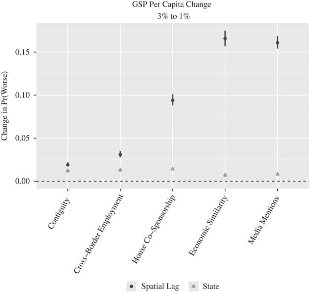
Fig. 1 Change in the predicted probability of selecting “worse” given a decrease (3–1 percent) in the spatial lag for change in gross state product (GSP) per capita across specifications of W Note: Vertical lines represent 95 percent confidence intervals. Dashed line depicts the null hypothesis test.
The results are quite consistent across the variety of geographic-, economic-, political-, social-, and elite-based specifications; in each case, the probability of respondents selecting “worse” increases in response to worsening economic conditions, both at the state and “local” level. As the vertical lines do not overlap the horizontal dashed line, we can conclude that each of the effects is statistically different from 0 at the 95 percent confidence level. In each case voters respond as one might expect to economic information, regardless of how it is contextualized.
While the effects are consistently positive, there is a great deal of variation in the magnitude of the changes. As the size of the economic shock stays the same across specifications (all the Ws are row-standardized), this variation in probability shifts is a result of how the Ws specify which states are connected and to what extent. Figure 1 shows that these spatial evaluations are much stronger in some cases than others, and the effects are grouped together in interesting ways. The second largest effect (by a hair) comes from the media contextualization measure, likely the most direct proxy for the distribution of economic information voters are likely to be exposed. Exerting nearly identical effects is the economic similarity measure, which connects states based on similarity of industrial production. Of course, we would expect (or at least hope) that similarity across economic sectors would be among the best connectivity measures when considering change in economic production—it is only natural that economic discourse regarding productivity weights the performance of other economies according to their similarity to the focal economy. Hence, agricultural states discuss the performance of other agricultural states more often and the performance of finance and insurance states less often. These results suggest that voters contextualize economic information, and when searching for sources of information they most often rely on economically similar states and those that the media identify as economic rivals. Geographic specifications—while providing the same inference regarding the direction of the relationship—underestimate the degree of contextualization that occurs.
A final observation is that the aggregated performance of other states influences economic evaluations to a greater extent than the performance by one’s own state in all of the specifications. The relative magnitude of the effects ranges from being slightly—though statistically—larger to exceeding the state effects by a magnitude of 8 (media mentions and economic similarity).
Model Comparison
While one of the central points of this manuscript is to argue for a theory-driven approach to connectedness in the aggregation of economic information and in the construction of SLX models more generally, there is substantial value in comparing our different specifications against each other and the national indicator to evaluate which, if any, provides superior explanatory power. First and foremost, if the national indicator provides the best fit, then many readers would be justified in doubting the value of this exercise. Second, tracing the variation in model performance can serve as a guide to future researchers as to which W matrix may provide the best leverage on their question, or what the tradeoff between predictive efficiency and theoretical match may be. Finally, and most interestingly, learning which weighting matrix provides better fit can help us to understand the process by which economic information is aggregated locally. If, for example, a cross-border employment weighting is outperformed by weighting based on the similarity of economic production (and it is), then we may conclude that economic production is much more salient in determining the distribution of economic information one gets exposed to than the proportion of citizens working in neighboring states. In other words, discovering which model provides the most explanatory power can bring us one step closer to discovering the nature of the distribution of economic messages from locality to locality, and therefore the root of the public’s economic beliefs.
Because our different measures are too highly correlated to all be included in the same model (Achen Reference Achen1985), we evaluate their relative fit by employing Clarke’s (Reference Clarke2003, Reference Clarke2007) “distribution-free” non-nested model selection test. In sum, the test evaluates which model is closer to the “true” data-generating process by comparing the individual likelihood estimates for each observation. More specifically, we compare one vector of recovered log-likelihood estimates from Model A with the vector of recovered log-likelihood estimates from Model B, and count the number of observations for which Model A’s log-likelihood estimate is smaller than Model B’s (indicating Model A provides better fit). Next, we calculate the probability of observing this count under the assumption that the models are equivalent (we refer to this probability as the “Clarke statistic”). In other words, our null hypothesis is that the models perform equally well, and therefore that the probability of any observation’s estimated log-likelihood in Model A is smaller than its estimated log-likelihood in Model B is 0.5; or, that the median difference in log-likelihoods is 0. The Clarke statistic is the probability of observing the recovered difference in fit between the models under this null.Footnote 13
We first conduct this test as originally prescribed by Clarke, by comparing the recovered likelihoods of each observation in our data across all of the models. We then execute a second version of this test—a bootstrapped out-of-sample prediction test that allows us to evaluate the sensitivity of our results to sample.
We first conducted Clarke’s in-sample test for all of our models and recovered a ranked ordering of the models’ explanatory power.Footnote 14 In Table 3, we describe this rank-ordering by displaying the difference in fit for rank-adjacent models. The “A<B” column displays the proportion of observations for which Model A provides better fit (smaller log-likelihood) than Model B and the “p” column displays the Clarke statistic, the probability of observing that proportion under the assumption that the models are equivalent, or, our certainty that Model A is closer to the “true” model or “true” data-generating process than Model B.
Table 3 Clarke Test of Specifications
The results of our second test are displayed in the final three columns. To generate these values we randomly draw four-fifths of the observations, estimate the models, and use the results to generate predicted values for the omitted one-fifth of the sample. We then compare the precision of the predicted values for each model pair, calculate the Clarke statistic, log it, and repeat the process 1000 times to build a distribution of Clarke statistic values. These distributions are described with their 0.025, 0.5, and 0.975 quantiles in the table.
The data are quite conclusive that Model A is superior to Model B in each pairing, save the comparison between the national indicator and the contiguity matrix—this comparison passes the in-sample test, but fails the out-of-sample test. There are several important takeaways from these results. First, all but one W specification provides significantly more explanatory power than the national indicator, suggesting that, even though the national indicator is likely the most reported economic figure, it nonetheless fails to capture the relevant distribution of economic messages in a particular locality in many cases, and therefore offers less explanatory power than alternative aggregations of economic information. As for the rank-ordering, the media messaging weights matrix provides the greatest explanatory power, followed by the economic similarity matrix, House co-sponsorship, the cross-border employment, and then simple contiguity. The largest divide is between the economic similarity weighting and the house co-sponsorship matrix. While it is certainly interesting that house co-sponsorship patterns provide better fit than the national indicator and geographically oriented measures (and one can certainly imagine an array of interesting theoretical explanations for economic perceptions that would utilize this aggregation), the clear dominance of the economic similarity and media-derived measures are the most interesting for present purposes because there are existing examples of theoretical research that propose voters employ such aggregation schemes and because of the normative salience of these measures.
We view the strong performance of the economic similarity measure as further evidence that the core of Ebeid and Rodden’s (Reference Ebeid and Rodden2006) argument is accurate. The data suggest that voters are substantially more responsive to economic production connectivity than geographic connectivity, connectivity as manifest in political preferences, or the national indicator. Not only does this finding comport with previous theoretical arguments, but it also has substantial normative implications. In short, this is the most salient type of connectivity in linking the economic fortunes of states. Production similarity should be among the better performing aggregation devices, because it is among the most salient drivers of local economic performance.
The superior performance of the media contextualization measure is similarly encouraging. Several previous studies of responsibility attribution explicitly note the role of the media in providing economic information to voters (e.g., Duch and Stevenson 2008) and we discussed the “pre-processing” role that Kayser and Peress (Reference Kayser and Peress2012) argue the media can play in the dissemination of economic messages earlier in the manuscript. Our findings support their arguments that the media play a pivotal role in determining the distribution of economic messages that voters may be exposed to. Indeed, we believe that the rank-ordered performance of the W matrices is less a function of their correlation to the true local economy than a function of their correlation to the distribution of media messages about the economy. Examine Figure 2, in which we display how the W matrices correlate to both the media-derived W and real local economic performance. The rank-ordering of the correlations to media matrix is identical to the rank-ordering of model fit recovered in Table 3. That is, the data suggest that connectivity as manifest in the similarity of economic production and House co-sponsorship are high-quality predictors of economic perceptions, not because they necessarily correlate well to local production and drive the local economic conversation directly, but because they drive the media narrative on economic productivity.
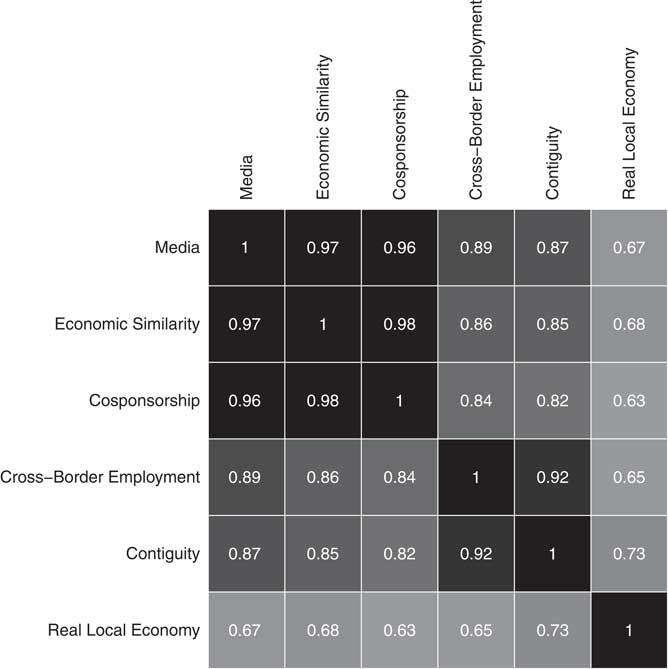
Fig. 2 Correlation of W matrices
Conclusion
Understanding the determinants of economic evaluations is of self-evident importance to the study of democratic accountability. In this manuscript, we have argued that the relevant distribution of economic messages citizens sample from when creating or updating their economic evaluations is likely to vary contextually as a function of localized economic discourse. Of course, versions of this argument have been made before by, for example, scholars interested in the role of partisanship in shaping economic evaluations (e.g., Evans and Anderson 2006) as well as those explicitly interested in the contextualization of economic information (Kayser and Peress Reference Kayser and Peress2012). But the connection we draw between this theoretical contextual variation and the empirical design is novel. In sum, we argued that, because economic discourse varies contextually, models of economic evaluations are effectively a special case of a broad class of spatial econometric models known as SLX models. Because of this, it is incumbent upon researchers to draw links between their theorized process of evaluation creation (or economic accountability) and local distributions of economic messages. We illustrate this by discussing two recent theories of economic accountability that stress the contextual nature of responsibility (Ebeid and Rodden Reference Ebeid and Rodden2006; Kayser and Peress Reference Kayser and Peress2012) and derive from them theoretically motivated schemes for aggregating the performances of subnational economies in an effort to approximate the distribution of economic messages from which voters draw their evaluations. We then evaluate the predictive power of these aggregations (and several others) against the current industry standard, the national indicator. We find that each of our aggregative schemes provided better model fit than the national indicator, including the more simple aggregations, like spatial contiguity. We also find that aggregating the performance of subnational economies according to similarity in economic production (Ebeid and Rodden Reference Ebeid and Rodden2006) or according to patterns of media contextualization (Kayser and Peress Reference Kayser and Peress2012) provides significantly more predictive power than any of the competing aggregation schemes and, of the two leaders, the media measure is the clear winner.
These results suggest that, even in our increasingly nationalized political culture, the distribution of economic information voters draw from varies substantially across contexts and failing to model this variability may substantially reduce model fit. Second, these results show that the type of interconnectivity that matters in structuring economic information transcends geographic proximity. This is particularly important because we believe geographic contiguity is a superficial type of connectivity in comparison with similarity in economic production; thus, the distribution of economic messages in a particular state seems to be driven by a more theoretically pleasing type of interconnectivity. It is also important because the lion’s share of SLX models to this point have relied on geographic contiguity to model interconnectivity, perhaps to their detriment in some cases.
Finally, we believe that this manuscript will help scholars recognize that they may be implicitly estimating SLX models and aid them in thinking carefully about how they specify the interconnectivities between observations, choosing a measure that provides a fit to their theory, and also motivate them to examine the robustness of their findings to those specification choices. We think that this conclusion is particularly apt for the spatial policy diffusion literature. The primary means of policy diffusion across states is typically assumed to be through geographical neighbors, and social learning theory provides a solid foundation for this assumption (Mooney Reference Mooney2001, 104–5). However, geography cannot be the only or even the most important causal mechanism spatially linking policy adoption (Neumayer and Plümper 2016). The type of interconnectivity that is modeled must correspond to the mechanisms of information flow or learning that the model suggests, which may or may not be captured with contiguity matrices. Indeed, we echo the concerns of Karch, who states that “one of the starkest shortcomings of existing state policy diffusion research is that it focuses almost exclusively on geographic proximity as the motivator of such lesson-drawing, at the expense of other plausible explanations” (Reference Karch2007, 56). We demonstrate the utility of a theory- and data-driven approach to specifying the weights matrices and are confident that those who study state policy diffusion will find these methods helpful.


