There is a long and rich tradition of using historical processes to explain political outcomes (Thelen Reference Thelen1999; Reference Thelen2000). Pierson (Reference Pierson2004) reminds us that politics occur in time, which is an undercurrent of classic literature in political science (Moore Reference Moore1966; Dahl Reference Dahl1971; North Reference North1981). Beyond simply acknowledging the importance of time, scholars have argued for the differentiation of duration, tempo, acceleration and timing (Abbott Reference Abbott1992, Reference Abbott2001; Mahoney Reference Mahoney2000; Pierson Reference Pierson2000, Reference Pierson2004; Page Reference Page2006; Slater and Simmons Reference Slater and Simmons2010; Grzymala-Busse Reference Grzymala-Busse2011). The unresolved debate over what affects the timing of democratization (Mansfield and Snyder Reference Mansfield and Snyder2007) represents a broader concern among scholars regarding how political processes are moderated by time. The challenges that this presents are twofold: the first is to identify different temporal processes qualitatively; the second is to involve them in empirical treatments. As Grzymala-Busse (Reference Grzymala-Busse2011) notes, it is important to distinguish temporal processes from causal mechanisms, as some causes may operate under specific temporal conditions. A process is outcome dependent if the outcome in a period depends on past outcomes or on the time period. If the long-run distribution of past outcomes matter, the process is said to exhibit path dependence (Page Reference Page2006). To this end, the notion of path dependence has been revived to address empirical problems related to ‘informative regress’ and increasing returns in political processes (Page Reference Page2006; Freeman Reference Freeman2010; Lin and Cohen Reference Lin and Cohen2010; Slater and Simmons Reference Slater and Simmons2010; Walker Reference Walker2010; Jackson and Kollman Reference Jackson and Kollman2012; Kreuzer Reference Kreuzer2013).
Existing approaches to handling time dependence include the use of multivariate statistical methods involving successive time points, factor analysis and cluster analysis. Yet each of these methods has the weakness that each time point is treated independently of others. Longitudinal methods are more capable of handling different forms of time dependence. In event history analysis, time refers to the length of time before a transition from one state to another. This treatment accounts for duration with precision, but neglects transitions between multiple categories. Time-series methods take time seriously insofar as what happens in one instant can be conditioned by prior moments. Autoregressive, integrated and moving average models also account for prior states and average effects. Such models are more appropriate for accounting the evolution and correlation of strictly continuous variables on frequent time points, but many social science data are categorical and contingent. Some of the most advanced models for time-dependent categorical data include hidden Markov models and higher-order Markov models. However, hidden Markov methods do not allow one to ascertain similarities between sequences or to easily handle a large number of varied sequences. As such, temporal problems remain in the empirical analysis of political phenomena, especially at the nexus of categorical data and time dependence.Footnote 1
Sequence analysis—which is more commonly found in sociology—is a method of processing sequence data, with sequences being defined as a series of states or events. It includes tools to code and format sequences, to compare them by pairs, to cluster and represent groups of similar order, to calculate specific statistics for sequences and groups of sequences, and to extract prototypical sequences. Sequences can be composed of a number of different units of time (for example, hours, days, weeks, months, years), whether they refer to states or events. States denote the properties or status of the unit of observation (for example, Republican, military dictatorship), while events denote a change between states (for example, holds elections, coup d’etat) (Blanchard Reference Blanchard2011, Reference Blanchard2013). Sequences made of events ignore duration and focus on the order of punctual experiences, while sequences comprised of states deal with both duration and order. For logical reasons, statistical sequences cannot mix states and events (Blanchard Reference Blanchard2011, Reference Blanchard2013). These receive slightly different treatments, though they are essentially equivalent from a statistical perspective. The full set of elements from which the steps in a sequence can be chosen is referred to as the alphabet (Blanchard Reference Blanchard2011; Gabadinho et al. Reference Gabadinho, Ritschard, Studer and Muller2011). A sequence, then, is a succession of elements chosen from an alphabet, where succession denotes order.
Sequence analysis (herein denoted SqA) refers to the systematic study of a population of sequences. This approach was originally used in computer science to detect dissimilarities between long strings of codes. Sociologists and demographers have used this approach to consider topics such as job careers and life trajectories (Brzinsky-Fay and Kohler Reference Brzinsky-Fay and Kohler2010), critical transitions from education to work to retirement (Abbott Reference Abbott1995), policy diffusion (Abbott and DeViney Reference Abbott and DeViney1992), patterns of violence (Stovel Reference Stovel2001), elite careers (Lemercier Reference Lemercier2005), legislative processes (Borghetto Reference Borghetto2014) and activism (Fillieule and Blanchard Reference Fillieule and Blanchard2011).Footnote 2 Though sequence analysis is very much alive in other social sciences, it is only beginning to be used in political science.Footnote 3 Most notably, SqA has been evoked in a recent symposium in political science on how historical time is conceived (Blanchard Reference Blanchard2013; Kreuzer Reference Kreuzer2013).
The application of SqA seems conceptually promising for explaining political phenomena at various levels of analysis. At the individual level, one might consider trajectories that involve electoral decision making, party positions, social status, political involvement and public opinion. It can also be a useful tool for analyzing the particular words, sentences and paragraphs invoked in political discourse. At the organizational level, one may focus on the development of parties, trade unions, activist groups and rebels. At the macro level, SqA can help explain the development of political regimes and how timing affects the transition to (or from) democracy. SqA can even supersede nations to explain patterns of international activity, such as the diffusion of norms, conflict behavior and large-scale geopolitical sequences.Footnote 4 As noted by Blanchard (Reference Blanchard2011), some of the primary objectives of sequence analysis are to describe and represent, compare and classify, identify dominant patterns, and explain and model sequences.Footnote 5 We briefly address each of these broad objectives below.
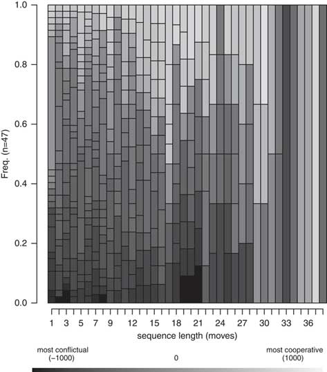
Treating as a sequence a string of related elements that is associated with a common unit allows one to visualize and consider how the elements are related. A standard way to visualize sequences is with a sequence index plot, in which sequences are stacked and temporally aligned (usually horizontally). A sequence density plot is similar to a sequence index plot. Rather than showing the sample of sequences, however, it sorts the elements that make up the alphabet by their frequency at each successive position. Examples of a sequence index plot and sequence density plot are shown in our application, below. Sequence frequency plots can also be used to display the most frequent sequences, each one with a bar of its successive states, in the order of their frequencies. An example of a sequence frequency plot is available in online appendix B.
The core of SqA lies in the algorithm used for distance comparison—that is, the metric by which sequences are quantifiably compared. Critical questions at the heart of dissimilarity calculation are which element of time should be preserved and how weights should be applied. There are several common metrics by which to compute sequence similarity. Some examples include Longest Common Prefix (LCP), Longest Common Subsequence (LCS) and Optimal Matching (OM) (Gabadinho et al. Reference Gabadinho, Ritschard, Studer and Muller2011).Footnote 6 OM is the most commonly used metric for sequence comparison (Elzinga Reference Elzinga2008).Footnote 7 By matching, it generates edit distances that are the minimal cost—in terms of insertions, deletions and substitutions—for transforming one sequence into another. The optimal matching algorithm compares two sequences state by state and determines the set of operations that would align them at the lowest cost, producing an n x n matrix of dissimilarity (or distance) between them. Once the dissimilarity algorithm and cost scheme are decided, there are a variety of ways in which one can analyze sequences through by using the resulting dissimilarity matrix. One method is to use cluster analysis to sort sequences into like groups, thereby enabling visual comparison.Footnote 8
Sequence analysis also has the capacity to search for sequences that share common subsequences. Subsequences refer to non-unit sections of sequences (that is, successions of two or more states or events inside longer successions). The more common subsequences two sequences share, and the longer these common subsequences are, the more similar the two sequences are. To search for patterns within a sample of sequences—read as subsequences—the LCS and LCP algorithms are useful tools. In addition, one can cluster sequences on the basis of optimal matching, and generate and rank the frequency of subsequences in a sample.
Finally, as a modeling technique, sequence groups created through hierarchical clustering can be included in cross-trabulations and logistic regression models.Footnote 9 Given a theory about order, one can also use a distance calcualtion to compute similarity to a theoretically important sequence, whether it is an example (case study) or an ideal sequence (hypothetical). By taking the distance values computed for each sequence in a sample, one has a continuous predictor of outcome that rests on the principle of order (Grzymala-Busse Reference Grzymala-Busse2011). Such an approach provides a direct test of whether, and to what extent, sequential theories about politics hold true.
By incorporating aspects of SqA into quantitative models, one can more easily quantify and test arguments about sequencing. Proponents of democratic sequencing, for example, assert that if reforms occur in the wrong order, then democratization can result in suboptimal outcomes such as empowering illiberal leaders, engendering violent nationalism, and instigating civil conflict and interstate wars. To the extent that the order of democratization matters, the probability of successful governance differs (Carothers Reference Carothers2007a, Reference Carothers2007b; Mansfield and Snyder Reference Mansfield and Snyder2007; Fukuyama Reference Fukuyama2011; Hobson Reference Hobson2012). The ability to quantitatively test such arguments—which are in part derived from extant arguments in qualitative comparative politics—would substantially advance the understanding of how politics as a process affects development.
Application: Crisis Bargaining Patterns
As a demonstration, we consider the effect of actors’ behavior in national crises. Our aim is to see whether different patterns of cooperation or conflict are associated with specific factors that pertain to a crisis. Do patterns of bargaining reinforce or undermine democracy, in that actors in different types of countries bargain in different ways? We focus on actors’ behavior during national crises because crises entail a “sequence of interaction” between actors (Snyder and Diesing Reference Snyder and Diesing1977) in “a noisy, dangerous, and unavoidable learning process” (Fearon Reference Fearon1992).
Our investigation entails assessing actors’ behavior across 47 crises in 12 countries. We selected 12 cases to represent different levels of democracy, transitions and predictability (Casper and Tufis Reference Casper and Tufis2003). First, we used the Polity IV scale to divide countries into democracies, autocracies and anocracies (countries that fell between these two regime types), with six as the threshold value (Marshall and Jaggers Reference Marshall and Jaggers2003).Footnote 10 We then coded each country as stable, transitioned or unstable over time, based on whether it remained in its respective category, moved unidirectionally to another category or experienced more than one transition during the period 1951–92.Footnote 11 The above decision rules led to five categories: stable democracies, cases that switched to democracy, countries that were unstable, cases that switched to autocracy and stable autocracies. Finally, we selected predictable and unpredictable cases based on the residuals from a naïve model of democracy (that is, the difference between a case’s actual and predicted levels of democracy) (Casper and Tufis Reference Casper and Tufis2003). A country-year was considered ‘predictable’ by the democracy model if its value fell within one standard deviation of the mean of the residuals.Footnote 12 As a result, the cases that were selected represent different countries with different levels of democracy and transition histories, which would be considered unpredictable and predictable according to a naïve model of democracy (Casper and Tufis Reference Casper and Tufis2003).
Once we selected the 12 cases, we identified crises that occurred, or were occurring, within the country from 1950–99. Our definition of a crisis follows Banks (Reference Banks1999) and can be of four types: riots, anti-government demonstrations, revolutions and guerilla warfare (see Online Appendix A). By definition, crises occur between the effective government and an opposition, which can have formerly been part of the government. Our decision to code moves as occurring between two actors draws on the unitary actor assumption, which treats one or more people or groups as a unified actor. Our use of the term actor refers to one or more people or groups who are united by explicitly stated shared goals. According to our framework, each crisis contains an actor representing the government, and a relevant opposition. Where this criterion is not met, we code it as a different crisis. Our investigation of the 12 countries resulted in 47 crises during the study period.
We detailed the reported events in Keesing’s World News Archives from the time the crisis began until the date that it ended, or from the start to the end of our window of observation. For each of the 47 crises in our 12 countries, we coded the actions (to which we refer as the ‘moves’) of each actor using the Intranational Political Interactions Conflict Scale (Davis, Leeds and Moore Reference Davis, Leeds and Moore1998) (Online Appendix A). The scale ranges roughly from 1,000 to –1,000 and differentiates between the types of actions that can be taken by an actor, ranking them according to cooperativeness (0 to 1,000) and ‘conflictualness’ (0 to –1,000).Footnote 13 Out of a series of political events, we denoted the most significant action (or verb) taken by each actor and assigned to it the corresponding number on the conflict scale. We began each series with the move of the actor acting on the part of the government, denoted by M t . M stands for the actor’s move and t represents the point in time of the move. We then coded the response of the opposing actor as M t+1. We continued to code the most significant response by each actor in the protracted series, thereby constructing a series of alternating moves between the two primary actors. The time reference by which we constructed the crisis sequences is internal as opposed to external (pertaining to how a sequence unfolds rather than calendar time). We are less interested in the duration of crises or the duration of spells in a crisis, and more interested in the order in which the spells in a crises occurred. Nevertheless, duration (sequences based on calendar time) can be accommodated by SqA.
Figure 1 shows a sequence index plot of the crisis sequences, whereas Figure 2 shows the sequence density plot of the same information. Each line represents a crisis in one of our 12 cases and is labeled with the name of the case and the crisis (for example, country_crisis name). There are 47 crises in our dataset, which vary in length from 4–38 moves. The average length of a crisis in our sample is eight states long. The most frequent state in our data is that of less to moderately negative events (IPI –100 through –500). This is true of both the mean and the modal state across sequences. The mean number of moderately negative moves in a sequence is six, while the next-highest occurrence is highly negative events, with a mean of four moves per series. Based on sequence averages, a randomly drawn series should be predominantly composed of moderately and highly conflictual moves. Neutrality is highest at the beginning and end of sequences, and the likelihood of cooperative moves generally increases with sequence length. As indicated by the frequency plot, virtually no two sequences are perfectly alike—the ten most common sequences represent, in effect, ten of our series. Online Appendix B provides additional descriptive figures on the crisis sequences.
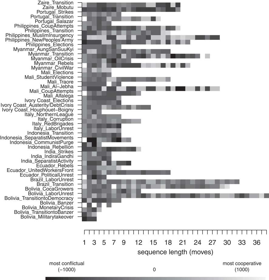
Fig. 1 Sequence index plot
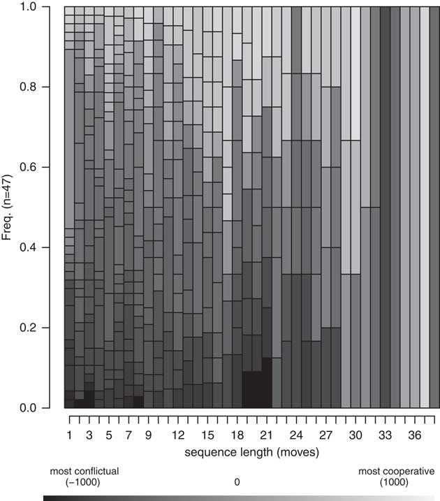
Fig. 2 Sequence density plot
We used the OM algorithm to calculate sequence similarity. The substitution
costs that we chose reflect the distance between states (for example, comparing
200 to –200 yields a cost of 400). We also set the insertion-deletion cost
arbitrarily high to ensure that all comparisons incurred substitution costs. To
better understand how to distinguish crisis bargaining patterns, we clustered
our sample into six groups using the Ward (Reference Ward1963) hierarchical clustering algorithm. Our choice of six clusters
was determined by rounding to the largest integer less than or equal to the
square root of our sample size (
 $$\sqrt {47} $$
≈6.85).Footnote
14
$$\sqrt {47} $$
≈6.85).Footnote
14
Given the considerable variation in the lengths of the crises, we calculated sequence similarity based on the first four moves of each crisis. This approaches accommodates the shortest crisis in our sample, such that crisis length has no effect on how the sequences are clustered.Footnote 15 The results shown here therefore focus on potential relationships between how crises begin (initial reciprocation) and features of the crises. The clusters created based on the comparing the first four moves of each crisis can be seen in Figure 3.
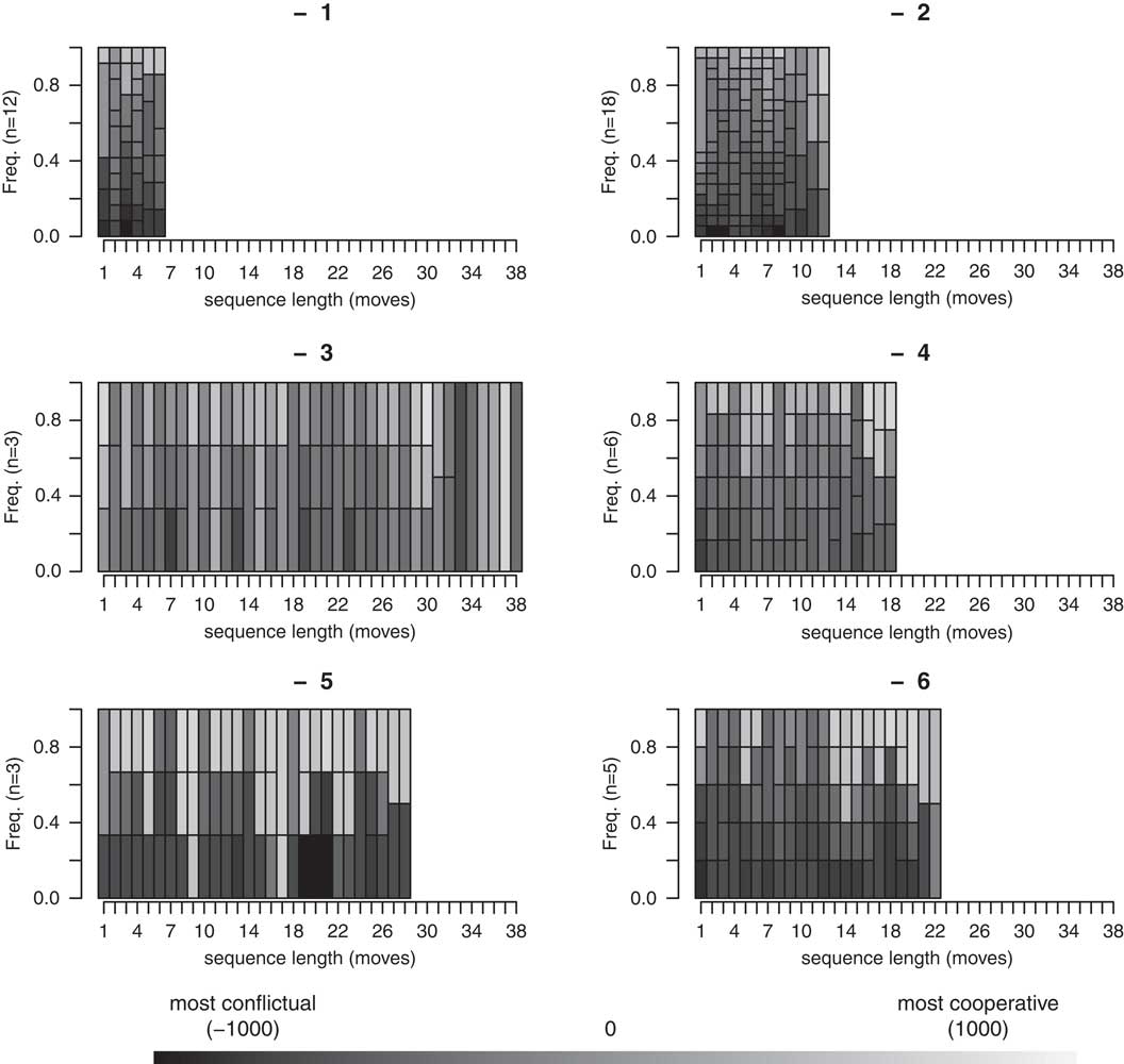
Fig. 3 Sequence density plot by cluster Note: using Ward (Reference Ward1963).
After clustering the crises based on how how they began, we sought to determine whether any factors are significantly associated with the clusters into which they had been sorted. In accordance with our theory, we test the following covariates: prior cooperation, shared interests, crisis origin and cohesiveness (Casper and Wilson Reference Casper and Wilson2012). If there was no prior crisis in our sample, or if the last crisis did not end on a cooperative note, we denoted the absence of Prior Cooperation with 0, and 1 if there was prior cooperation. Similarly, we coded Shared Interests as a dummy variable indicating whether or not the government and opposition had shared interests (that is, wanted a similar outcome or had a similar goal). For example, during the Clean Hands investigation in Italy, both the government and opposition had a vested interest in maintaining normal government functions, unlike those involved in the Northern League crisis. Endogenous Crises were coded as 1 if the problem over which the actors were bargaining originated within the country. Myanmar_Oil Crisis, for example, was created by fluctuations in the worldwide price of oil. Similarly, the crisis Italy_Labor Unrest originated with the end of the Bretton Woods system and increasing oil prices. Finally, we coded the variable Cohesiveness by denoting, at each move, whether either of the two actors encountered significant in-group opposition. An example of a lack of cohesiveness can be found in Italy_Northern League, when Umberto Bossi radicalized his discourse and withdrew from the coalition government, thus polarizing the league and losing support.
We were also interested in identifying whether the beginning of a crisis was affected by the issue over which the crisis began. Based on our a priori knowledge of each crisis, given by its unique name, we identified the general ‘theme’ of each. We denoted each crisis by one of the following subject labels: coups, civil war, economic crisis, elections, government specific, leader specific, labor, protests, purges, rebels, separatists and transition. Finally, we also examined whether clusters were significantly related to crisis length. By virtue of our specification (comparing the first four moves of each crisis), crisis length should not have affected clustering. To the extent that they are related, it therefore suggests that how the crises began affected how long they lasted.
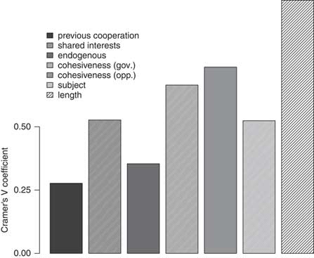
Cramér’s V is used when the number of possible values for two categorical variables is unequal, yielding a different number of rows and columns in the data matrix. Thus, this correlation measure is appropriate for measuring the association between cluster number and each of our dummy variables (Cramér Reference Cramér1946). Like other measures of correlational association, Cramér’s V ranges from 0 (no relationship) to 1 (perfect relationship). The p-value associated with the Cramér’s V statistic indicates the probability that the cell counts are due to chance. For each of the seven covariates, the p-value associated with the Cramér V statistic is below 0.01, indicating that none of the associations is random.
Figure 4 shows a plot of the Cramér’s V statistic associated with each variable and the clusters. According to Crewson (Reference Crewson2012), a Cramér’s V statistic greater than 0.5 characterizes a high level of association between two variables. The results suggest that previous cooperation is not strongly related to the manner in which crises were clustered, and that endogenous crises are not differently grouped. Shared interest is strongly associated with how crises were clustered, however, which suggests that the order in which a crisis is initiated is affected by the correspondence of the actors’ goals. Actor cohesiveness, both government and opposition, also seems to affect how a crisis begins.
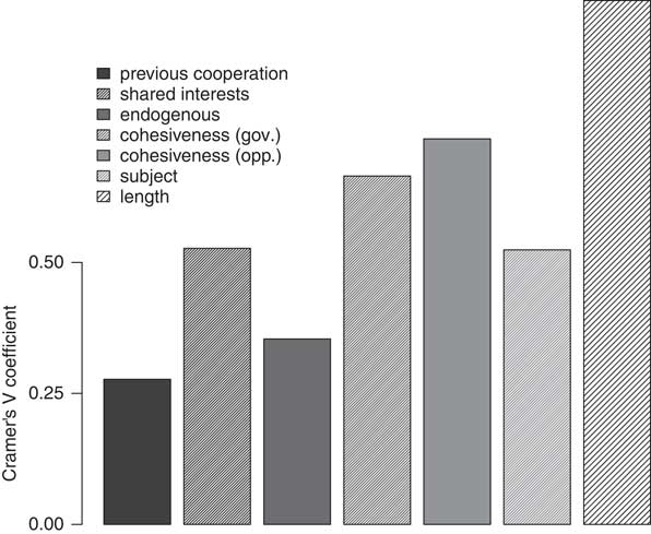
Fig. 4 Bar plot: Cramér V coefficients, by covariate Note: above 0.50 denotes threshold for strong association.
Interestingly, the general theme of a crisis is also strongly associated with cluster number. This may suggest that how a crisis begins is also affected by its nature (what is the crisis about?). Nevertheless, the level of association between cluster and subject is similar to that of shared interests. It may reflect the fact that some issues are inherently zero sum, such as bargaining over secession. Most notably, the clusters are strongly associated with crisis length. Though we intentionally prevented crisis length from affecting how crises were clustered, there is still a strong association. This suggests, therefore, that how crises begin affects their duration.
Our investigation of actors’ behavior across 47 crises in 12 countries focused on the “sequence of interaction” between actors (Snyder and Diesing Reference Snyder and Diesing1977). Using SqA, we demonstrated that our sample of crises divides into unique subgroups with common bargaining patterns and features. The clusters, which we discerned based on pattern commonalities, are significantly associated with shared interests, crisis origin and actor cohesiveness. Bargaining patterns are thus affected by known factors in a crisis, which reinforce or undermine democracy. While just beginning to be applied to a larger empirical agenda, our results bode well for explaining a nuanced dimension of bargaining (order of action) and for developing a new approach to studying political sequencing.
To add to this agenda, scholars must carefully consider the assumptions and decisions that are necessary to compare qualitative sequences quantitatively. Doing so will serve to better explain how patterns of bargaining reinforced or undermined democracy, and will more broadly yield exciting new insights into complex political processes. Further extensions of this work explore bargaining sequences through comparative historical analysis. As an example, however, it illustrates the promise of SqA applications in political science to questions of order and sequence.
Robustness
Though OM is just one of several types of sequence analysis algorithms (methods for comparing pairs of sequences), almost all applications of SqA in the social sciences have used the OM algorithm (Abbott and Tsay Reference Abbott and Tsay2000; Hollister Reference Hollister2009). Little is known about the robustness of OM classification, however, which limits its utility beyond description (Hollister Reference Hollister2009). A number of studies have added confidence to the validity and reliability of the OM algorithm. Abbott and Tsay’s (Reference Abbott and Tsay2000) review of social science research utilizing OM alignment in SqA evaluates nearly all articles, conference papers and dissertations using the method at the time. They discuss issues related to OM alignment and how various authors have dealt with them. They conclude that OM is a legitimate classification method that is not based on a probability model of sequence generation, and that it produces reliable and valid results. Previously, Forrest and Abbott (Reference Forrest and Abbott1990) had tested the impact of intercoder reliability on OM results. The authors had five coders independently code sequence data that they had analyzed in previous work (Forrest and Abbott Reference Forrest and Abbott1986). The authors found that coding decisions and the level of detail varied by coder. Analyzing the variation by applying OM and using data-reduction techniques, however, they found that the aggregated results based on each dataset resembled each other. Their robustness test also suggested the reliability and validity of OM for divergent datasets. Halpin (Reference Halpin2010) also addresses the critique that the OM algorithm is inadequate for analyzing episodic data (data for which the length of time spent in each state also matters). Modifying the algorithm to make it sensitive to spell length, the author demonstrates that standard usage of OM is reasonably robust to continuous-time sequences.
Existing studies that take the robustness of OM into account have demonstrated the ability of OM to accommodate both continuous and discrete-time data, and that it is relatively unaffected by intercoder reliability. Our introduction and application of SqA also aims to contribute to robustness tests of the algorithm. Beyond encouraging its use and adaptation to suit the needs of political science research, we also want to establish some of the current limits of the application. In an attempt to shed light on the limitations of SqA through the use of OM for political science research, we present the results of a simulation exercise in which we subjected the OM algorithm to a series of robustness tests. Primarily, we examine the extent to which OM is affected by error, which is a common concern for social scientists (Adcock and Collier Reference Adcock and Collier2001). We demonstrate that the statistical logic undergirding simple matching algorithms is sufficient to handle a number of problems that affect social science data. The value added of such tests is that they establish confidence in OM’s ability to identify dominant patterns in incomplete or erroneous data, which surpasses that of human coders. Though we recommend a healthy skepticism regarding its use in political science research, our tests confirm the validity and reliability of OM as a tool for analyzing sequences. We also comment on its sensitivity to sample size, subsequences and disproportionate sequences.
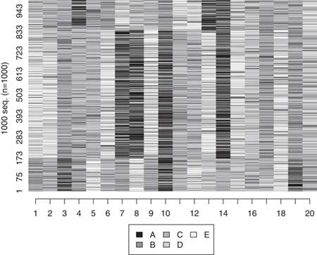
To set up the simulation exercise, we constructed known parameters of a latent concept by performing 1,000 random draws from a normal distribution and then associated them with three discrete categories (see Online Appendix C). We associated each category with a particular sequence that was 20 moves long, constructed based on five possible states (an alphabet of five). In each robustness test, we affected the sample with some form of error and then applied OM and clustered the sequences into three groups. For the purpose of this exercise we chose to use an insertion-deletion cost of 1 and a substitution cost of 2. This is the most common decision rule among studies that use SqA, and the choice to apply a cost of 2 to substitution reflects the combined costs of inserting and deleting a state, which both cost 1.
If we had perfect information about the sequences, the OM algorithm would sort them into perfect predictors of y. That is to say, when we apply the OM algorithm and cluster the sequences into three clusters, cluster assignment perfectly sorts the sequences into three homogenous groups. As social scientists, however, we know that there is likely error in our data, such as measurement error, systematic biases, inter-coder unreliability and random error (noise). As such, in our robustness check of the OM algorithm we consider some of the major sources of error that can arise in analyzing political science data.
In the first test, we introduced systematic error. This was accomplished by randomly selecting a cross-section (column) of data and randomizing everything in that column. This would be akin to having a time period of data in which a global shock affected all reported values (for example, war, natural disasters). We incrementally increased the amount of systematic error in the data from 1 to 20 columns, the total number of moves. We found that the OM algorithm is capable of nearly perfectly classifying sequences in which up to half of the data have been affected by systematic error, as shown in Figure 5 (see also Online Appendix C). Beyond this amount of systematic error, the OM algorithm begins to falter. The OM algorithm is thus capable of handling a large amount of error if there are missing or incomplete moves affecting the entire sample of sequences.
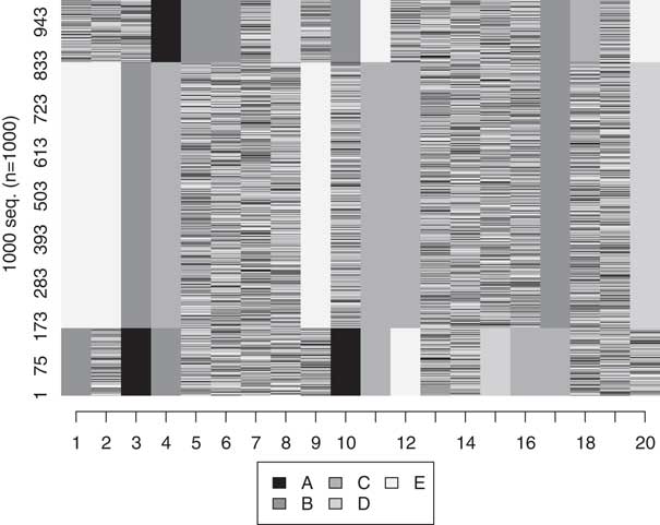
Fig. 5 Sequence index plot: simulated sequences Note: 0.5 affected by systematic error.
Second, we allowed the lengths of the sequences to differ. For each observation (row of time-series data), we selected a number of states between 1 and 18 to randomly delete from sequences in our simulated dataset, thereby creating samples with sequences of different lengths. A related example of this issue would be having data on subjects with different rates of survival/mortality (for example, presidents, regimes). The OM algorithm can handle differences in lengths of up to about 65 percent of the original length before it begins to classify them differently. Put another way, for a sample of data that is a maximum of 20 moves long and composed of five different states, the OM can fairly easily compare them with sequences that are 7 moves long (a difference of 13). Third, we changed the dimensions of the data to create four datasets that differ by the number and length of the sequences. The different dimensions of the datasets (expressed as rows by columns) that we created were 10×100, 100×100, 1,000×10, and 1,000×100. Out of necessity, we affected half of each dataset with systematic error. When we applied the OM algorithm, we discovered that this method was particularly sensitive to the overall length of sequences, as opposed to the number of sequences. Thus the OM algorithm works best for longer sequences and is not affected by the number of sequences. As expected, the method is best suited for time-series over cross-sectional applications.
Fourth, we introduced random error. This problem is commonly expected if there is ‘noise’ in the data, most likely due to missingness. As this issue is perhaps the biggest concern of social scientists, we randomly selected from 1 to 20,000 observations (the number of simulated observations) and replaced them with a random selection. In Figure 6, half of the dataset has been randomized. The OM algorithm perfectly handles up to 12 percent random error before it begins to misclassify the sequences with some probability. One can think of this variability as forming confidence intervals over the range of random error, although the algorithm seems fairly robust to a large proportion of random errors. Figure 7 shows how well the OM algorithm classifies sequences that are 20 states long, with increasing random error. In the above example (in which where half of the data was randomized) the OM algorithm correctly classified about 70 percent of the sequences.
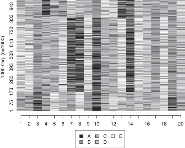
Fig. 6 Sequence index plot: simulated sequences Note: 0.5 affected by random error.
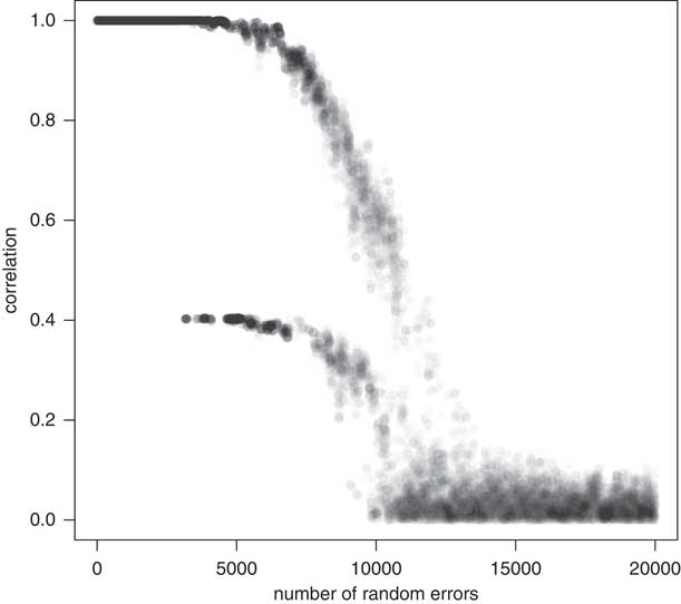
Fig. 7 Correlation plot: simulated sequences with increasing random error Note: using OM.
Finally, we repeatedly substituted within our sample a subsequence that was five states long to discern whether the OM algorithm would be misled by alternative patterns in the data. Surprisingly, the introduction of this new subsequence to a dataset that had longer common subsequences had no effect on classification. This suggests that pattern-matching algorithms prioritize dominant patterns at the expense of subsequences that might be attractive to human coders. Thus researchers interested in identifying ‘tempo’ should be aware of how they look for subsequences in the data (Blanchard Reference Blanchard2013).
Based on our robustness tests of the OM algorithm, we determined that it can handle a great deal of systematic error, differences in length, random error and even ‘misleading’ subpatterns in the data. Nevertheless, the algorithm is clearly not without flaws. What is more, its ability to compare sequences is diminished in the presence of more than one of these problems. These are issues that must be considered when using the metric to represent sequence similarities. Scholars who are interested in pursuing the use of sequence analysis in political science—primarily through the use of the OM algorithm—can be fairly confident about the systematic and random error in their data and secondary subsequences, and more wary of sequence length and the differences in length between sequences.
Regarding the use of clustering algorithms as a complement to SqA, we assert that sequence clusters can be thought of as latent classes. The latent classes created by clustering are derived from the sequence from which ‘like’ groups emerge. To this end, clusters created on the basis of a distance metric such as OM can be used as the dependent variable (for example, what determines whether an observation develops into Y?) or the independent variable (how do like sequences affect Y)? There is, of course, no standard method for discerning groups from the distances calculated by OM. There are a variety of ways in which clusters can be calculated. One approach would be to try various clustering methods and to select the method that has the biggest impact on model fit. It is also possible to calculate the similarity of each sequence with its assigned cluster (and to treat the ‘worst-fitting’ sequences as outliers) as another form of robustness check when using sequences or clusters in statistical models. The impact of clustering methods on predictive accuracy is nevertheless a separate topic—clustering is but one way to utilize the information produced by matching algorithms such as OM.
A superficial test of the robustness of the OM algorithm for SqA of flawed data shows surprisingly positive results. Fortunately, its use can be dramatically improved by considering (and attempting to mitigate) each of these issues in turn. Furthermore, selecting costs that are more theoretically motivated, or which aim to mitigate data problems, can make the analysis even more accurate. Abbott and Tsay (Reference Abbott and Tsay2000) highlight the need to test the effects of different cost schemes on OM classification.Footnote 16 An option that is just beginning to be explored, and which can further enhance OM, is how to apply weights to states about which one is more confident.Footnote 17 Another issue that we did not explore here is the effect on OM of increasing the number of states that comprise the alphabet. That is, when considering the ability of OM to correctly identify dominant patterns, scholars should consider the relative impact of the size of the alphabet. As a general rule, however, the more parsimonious the better. As is the case with all statistical models, one leverages nuance for generalizability.
In summary, our exercise undergirds our introduction of SqA by demonstrating that a common procedure for comparing sequences is fairly robust to a number of problems, and that it is thus a promising statistical technique for political science research. Further development of the OM algorithm offers to contine developing the study of sequences and dominant patterns in political science. We encourage political scientists to approach the method with a healthy degree of skepticism, but also to note the logical simplicity and transparency of OM as a means of comparing and quantifying the sequential nature of political phenomena.
Conclusion
Our brief description of SqA highlights how it can be used in political science to bridge the gap between qualitative arguments about order and sequence and quantitative methods. SqA methods are compatible with both qualitative and quantitative approaches. As an approach, it is simple, flexible and easy to interpret. It provides a simple yet sophisticated way to test sequencing, and allows for a great deal of flexibility without a substantial loss in degrees of freedom. It also provides easy-to-interpret clusters. As we demonstrated in the robustness tests of OM, however, the matching algorithms that are at the core of SqA can misclassify with some probability. This feature can perhaps be better exploited in the future. All the same, using clusters derived from a distance metric is equivalent to adding dummy variables to account for the uniqueness of sequences. It is not necessarily more theoretically appealing, but SqA does provide some empirical credibility to such claims. With SqA, there is also some probability of obscuring ‘true’ patterns in favor of dominant themes in discrete data. The OM algorithm is obviously sensitive to different forms of error, the extent to which we have begun to uncover. Nevertheless, SqA (and the distance metrics by which to conduct it) are still in development and show surprisingly robust results.Footnote 18
For the benefit of expanding political science research on sequences, future work should aim to compare the OM algorithm to different metrics such as the LCP and LCS, compare the impacts of different types of error and perhaps use this information to construct a measure of uncertainty (other than entropy) regarding the distance values that such metrics produce. As an empirical approach, however, SqA constitutes a promising agenda for quantitatively evaluating time- and order-dependent information. More broadly, however, this approach encourages a renewed focus on the types of time dependence and ways to model them in political science (Abbott Reference Abbott2001; Pierson Reference Pierson2004; Page Reference Page2006; Grzymala-Busse Reference Grzymala-Busse2011; Jackson and Kollman Reference Jackson and Kollman2012).