The formation of minority governments in parliamentary systems constitutes one of the most intriguing paradoxes in the study of coalition building. Parliamentary systems operate on the principle that the executive’s survival in office hinges on the (tacit) support of a majority in parliament. Yet, by definition, minority governments obtain majority support by allocating cabinet positions to a set of parties with only a minority of seats in parliament. In fact, as many as one-third of all governments formed during the post-WWII era in Western Europe were minority governments, while countries like Denmark or Norway have been governed almost exclusively by minority cabinets. Why do political parties support (or tolerate) minority governments without receiving cabinet portfolios? My goal in this study is to develop a parsimonious, yet general theory, that accounts for variation in the incidence of minority governments across parliamentary systems. This theory has its origins in the bargaining models of Austen-Smith and Banks (Reference Austen-Smith and Banks1988) and Baron and Ferejohn (Reference Baron and Ferejohn1989). It is distinguished from these studies and much of the existing literature because of the simultaneous incorporation of three requirements I deem essential for a theory of minority governments. In the remainder of this section, I first motivate these requirements, then describe the main findings and relate them to the literature on government formation.
Any attempt to understand minority governments brings us squarely in the realm of coalition theories and the literature spawned by William Riker (Reference Riker1962) and his “size principle,” the proposition that observed coalitions should be the smallest necessary to win and no larger. An important qualification to Riker’s dictum is that the literature often uses different criteria to measure the size of winning coalitions. For example, in abstract theories of coalition formation coalition size may be defined as the number of voters that support a particular agreement. As long as we maintain the assumption that cabinets must enjoy the (tacit) support of a majority in parliament, that criterion has no bite in the case of government formation because it automatically classifies all governments as majority governments. The phenomenon to be explained when it comes to minority governments is coalition size as measured on the basis of the observed agreement, specifically the share of cabinet portfolios controlled by parties that participate in the cabinet. It is thus essential for a theory of minority governments that (a) the portfolio allocation must be modeled as an explicit component of the government formation agreement.
Of course, government formation agreements determine both the allocation of cabinet posts as well as the policies to be pursued by the cabinet. While the electorate may not have preferences over the portfolio allocation per se, parties and individuals within parties certainly compete with each other over the allocation of cabinet posts. All else equal, it is natural to assume that political parties desire larger fractions of cabinet portfolios. Indeed, minority governments are paradoxical because cabinet positions are presumed desirable. I thus impose a second requirement that (b) a political party’s utility increases with larger share of cabinet portfolios for any given policy pursued by the cabinet. I emphasize that this assumption does not preclude the possibility that parties’ utilities from cabinet office may vary across countries, or over time, nor does this assumption speak in any way to the relative significance of parties’ office and policy aspirations.
The third requirement I impose is to (c) avoid dimensionality or other a priori restrictions on the agreement space over which political parties bargain. First, this requirement ensures that any conclusions do not rely on the common but special assumption of a one-dimensional policy space, which typically entails equilibrium properties that do not hold in higher dimensions. Importantly, as a result of this generality, the policy agreements in my model can represent the multitude and variable nature of decisions reached by the coalition partners on any sphere of the public domain (of course, other than the explicit allocation of the cabinets) ranging from, for example, the content and timing of new legislation on health care or taxation to the appointment and degree of discretion and control of the management of public utility companies, etc. I also avoid ad hoc a priori restrictions on the types of agreements that can be attained by particular coalitions, modeling the set of feasible proposals as a continuum. As a result, a formateur that would barely lose an investiture vote because of the objection of one of the intended coalition partners, can achieve the formation of this cabinet by granting an extra concession (in the form of cabinet portfolios or policies) to the objecting party.
Can minority governments be obtained in equilibrium while maintaining requirements (a), (b), and (c) above? I show that the answer to this question is almost always in the affirmative: minority governments emerge with positive probability when political disagreement or policy polarization among bargaining parties is marked relative to the importance of utility obtained by holding cabinet office. However, only majority governments form when policy disagreement is limited. Note that I qualify the statement of the result by “almost always” because it is possible to construct otherwise unspectacular examples in which the stated comparative static does not hold. In Theorem 2 I show that these examples constitute singularities that obtain only for knife-edge configurations of parameters.
The mechanism that links policy disagreement with minority governments can be best understood by considering the trade-off faced by the potential coalition partners of a formateur party. A party rejecting a proposed government agreement faces the risk that a coalition excluding this party will form instead, implementing a policy that is less desirable than the agreement on the table. When political parties are ideologically polarized, these potential subsequent policy agreements can be quite costly, thus rendering it more likely for parties to grant their consent to the formateur’s policy program without receiving any cabinet posts.
Note that in this mechanism minority governments emerge when a formateur’s party is in a position of strength vis-à-vis its coalition partners. Thus, although public commentary often associates minority governments with an impaired ability to pass their legislative program in parliament, in the present analysis these governments are certainly capable of mustering support from parties outside the cabinet in order to implement their policy program. In that regard, the present study adds to the arguments of a number of scholars, for example, Strom (Reference Strom1990), Tsebelis (Reference Tsebelis1995), etc., who similarly conclude that minority governments can be stable and viable governing solutions.
The main finding of this analysis linking minority governments with significant policy disagreement is consistent with anecdotal evidence for the prevalence of these governments across a number of countries. For example, minority governments in Israel are often associated with the existence of significant tensions over issues of national security and secularism among political parties represented in parliament. Similarly, minority governments are more likely in Scandinavian countries where political disagreement is marked, and where strong norms of meritocracy in the public sector and a long tradition of scrutiny of the government by independent bodies limit the private value of holding a cabinet post. I discuss more systematic empirical evidence in the “Minority governments” section. Note, though, that these empirical accounts and the proposed theory simply rely on the presence of significant ideological disagreement relative to the value of cabinet office in these countries, and do not imply that cabinet positions are not valued by the politicians in these countries.
Before I proceed with the analysis, I review related theoretical contributions with an emphasis on aspects in which they differ from the present study. Minority governments have been associated with policy polarization in one of the earliest accounts of the phenomenon to appear in the comparative politics literature by Dodd (Reference Dodd1976). In his account, though, the connection between policy polarization and minority governments is almost assumed. It amounts to an inability of polarized parties to participate in the same cabinet. Furthermore, minority governments of that flavor are expected to be of short duration (e.g., Powell Reference Powell1982, 142). Perhaps the earliest attempt to formalize a connection between policy polarization with minority governments is that by Itai Sened (Sened Reference Sened1995, Reference Sened1996). He considers a model with both policies and cabinet portfolio allocations and shows that equilibrium minority governments emerge when led by a large, centrally located party, and when other parties are significantly ideologically polarized (Sened Reference Sened1995, 292, theorem 2; Sened Reference Sened1996, 361, theorem 3). The main differences between Sened’s theory and the present study are, first, that his analysis relies on the assumption that parties incur a policy-related payoff only when participating in government. This assumption is consequential as it adds a policy “cost” (in Sened’s terminology) to parties that participate in the cabinet, thus facilitating minority governments. In contrast, I assume that parties receive policy payoffs from the implemented government agreement whether the party receives cabinet portfolios or not. Second, contrary to Sened’s theory, in the present study minority governments may emerge even if there exists no party in a central dominant location—as is the case in Example 1. Finally, Sened uses a static cooperative solution concept while the present analysis is non-cooperative, so that parties’ willingness to support different government types are formed endogenously on the basis of expectations of future play.
The bargaining process of government formation I assume falls in the tradition of sequential bargaining games initiated by Rubinstein (Reference Rubinstein1982), and was introduced in political science by Baron and Ferejohn (Reference Baron and Ferejohn1989). They study a divide-the-dollar game, and their model produces no minority governments if we interpret the division of the dollar as the division of cabinet portfolios. In a similar bargaining space, Baron (Reference Baron1998) considers a dynamic model with an exogenous random status quo in which minority governments are preferred by the formateur but do not form in equilibrium. Baron (Reference Baron1991) considers bargaining over a two-dimensional ideological space, but his analysis is silent on the emergence of equilibrium minority/majority cabinets, as he does not make portfolio allocations an explicit choice among bargaining parties.
Using cooperative solution concepts, Laver and Schofield (Reference Laver and Schofield1990), Laver and Shepsle (Reference Laver and Shepsle1990), and Austen-Smith and Banks (Reference Austen-Smith and Banks1990), all make the assumption that parties only care about policies and that cabinet portfolios accrue no independent office-holding payoffs. All three contributions reach the conclusion that minority governments may emerge when the policies pursued by these cabinets are invulnerable or core policies.Footnote 1 While Laver and Schofield assume that bargaining parties may consider a continuum of possible policy agreements, Laver and Shepsle and Austen-Smith and Banks restrict possible policy agreements to a finite number of credible (according to these authors) policy alternatives for each coalition. Existence of a core or stable government is more likely under these restrictions, but is not generally guaranteed without additional restrictions on the dimensionality of the policy space.Footnote 2
Diermeier and Merlo (Reference Diermeier and Merlo2000) derive conditions that induce or preclude minority governments in a model that also addresses the stability of these governments. They work with three parties and a two-dimensional policy space, identical to that of Example 1 in the present study, but assume that utility is transferable. These authors define the set of parties in the cabinet as the “proto-coalition” that determines the eventual government agreement, but the allocation of cabinet office to parties in this proto-coalition is not explicit. Specifically, an agreement in their model is a policy and a set of positive or negative transfers across parties. Note that positive transfers may be made to parties outside the proto-coalition (which by assumption are not in the cabinet) and negative transfers to parties inside the proto-coalition (which by assumption receive cabinet portfolios in addition to any utility from the policy implemented by the government). Such transfers include items (e.g., changes in the management and multiparty oversight of public utilities) that in the present study are modeled as part of the multidimensional policy component of the government agreement.Footnote 3 Bandyopadhyay and Oak (Reference Bandyopadhyay and Oak2008) consider a single period coalition formation model, assuming that formateurs propose one among a finite number of coalitions, with the agreement to be implemented by any coalition restricted to an exogenously fixed compromise.
A number of authors consider non-cooperative government formation models with assumptions related to those in the present study. The modeling framework for government formation used in the present study has its origins in the paper of Austen-Smith and Banks (Reference Austen-Smith and Banks1988), who consider a model of both elections and post-election bargaining that takes place among three parties that must both split cabinet portfolios and determine a policy drawn from a one-dimensional space. In their model, minority governments emerge in bargaining subgames that are not reached in equilibrium. Related three-party, one-dimensional models are analyzed by Kalandrakis (Reference Kalandrakis2000) and by Cho (Reference Cho2014), the latter model being dynamic with an endogenous status quo and elections. In addition, part of the results in Morelli (Reference Morelli1999, 816, theorem 4) concern a similar model without equilibrium minority governments. Jackson and Moselle (Reference Jackson and Moselle2002) study a version of the same bargaining model as in the present analysis with policies restricted in one dimension and focusing on party rather than government formation.
I now proceed to the main part of the analysis. I first present the model. Next, I show that this model produces majority governments with probability one in the absence of significant policy disagreement. In the penultimate section I establish the advertised result concerning minority governments, and further discuss its interpretation. I conclude in the last section. All proofs have been relegated to an Appendix.
Government Formation Bargaining
Consider a parliament consisting of n≥3 parties and denote the
set of these parties by N={1, … , n}. Let
s
i
>0 denote the share of seats corresponding to party i
and assume that no party controls a parliamentary majority, that is,
 $\mathop{\sum}\nolimits_{i\,=\,1}^n {s_{i} {\,=\!1}} $
and
$\mathop{\sum}\nolimits_{i\,=\,1}^n {s_{i} {\,=\!1}} $
and
 $s_{i} \leq {\textstyle{1 \over 2}}$
for every party i. The formation of a
government requires an agreement on a policy x∈X
and on the allocation of portfolios, which I represent as a vector
$s_{i} \leq {\textstyle{1 \over 2}}$
for every party i. The formation of a
government requires an agreement on a policy x∈X
and on the allocation of portfolios, which I represent as a vector
 $${\bf g}\,{\rm =}\,(g_{1} ,\,g_{2} ,\,\,\ldots\,\,,\,g_{n} )\in {\Bbb R}^{n} $$
that satisfies g
i
≥0 for each party i and
$${\bf g}\,{\rm =}\,(g_{1} ,\,g_{2} ,\,\,\ldots\,\,,\,g_{n} )\in {\Bbb R}^{n} $$
that satisfies g
i
≥0 for each party i and
 $$\mathop{\sum}\nolimits_{i\,=\,1}^n {g_{i} {\rm =}G{\rm \,>\, }0} $$
. I assume the policy space X is a convex and
compact subset of d-dimensional Eucledian space
$$\mathop{\sum}\nolimits_{i\,=\,1}^n {g_{i} {\rm =}G{\rm \,>\, }0} $$
. I assume the policy space X is a convex and
compact subset of d-dimensional Eucledian space
 $${\Bbb R}^{d} $$
, d≥1, and encompasses all the agreements in
the public domain (other than the allocation of cabinet posts) that can be
pursued by any cabinet. Accordingly, I define a government as
follows.
$${\Bbb R}^{d} $$
, d≥1, and encompasses all the agreements in
the public domain (other than the allocation of cabinet posts) that can be
pursued by any cabinet. Accordingly, I define a government as
follows.
Definition 1: A government is a pair (x, g) consisting of a policy x, and an allocation of cabinet portfolios g.
A government must receive the support of some coalition of parties that jointly
control a majority of seats in order to be invested, that is, it needs the
support of a winning coalition C⊆N such that
 $\mathop{\sum}\nolimits_{i \, \in \, C} {s_{i} {\rm \,>\, }{\textstyle{{\rm 1} \over {\rm 2}}}} $
. I distinguish minority governments from majority governments
using the default empirical criterion, that is, whether cabinet portfolios are
allocated only among parties that control a minority of seats in
parliament.
$\mathop{\sum}\nolimits_{i \, \in \, C} {s_{i} {\rm \,>\, }{\textstyle{{\rm 1} \over {\rm 2}}}} $
. I distinguish minority governments from majority governments
using the default empirical criterion, that is, whether cabinet portfolios are
allocated only among parties that control a minority of seats in
parliament.
Definition 2: A government (x, g) is a minority government if
the set of parties that receive a positive share of cabinets is not a
winning coalition, that is, if
 $\mathop{\sum}\nolimits_{i{\rm \, :\, }g_{i} {\rm \,>\, }0} {s_{i} \leq {\textstyle{1 \over 2}}} $
.
$\mathop{\sum}\nolimits_{i{\rm \, :\, }g_{i} {\rm \,>\, }0} {s_{i} \leq {\textstyle{1 \over 2}}} $
.
Of course, if a government (x, g) is not a minority government, then it is a majority government. I emphasize that a minority government must still be approved (or tolerated) by a winning coalition.
Bargaining among the parties takes place according to the following procedure. In each period t=1, 2, … before the attainment of an agreement party i becomes the formateur with probability p i and proposes a government. If this proposal is accepted by a winning coalition, the game ends with the formation of that government. Otherwise, the game moves to the next period and continues as above until an agreement is reached. I impose mild restrictions on the probabilities with which different parties become formateurs that take one of two forms. The first restriction, assumption (M1), requires that every party, that is not a dummy party, may become a formateur with positive, though possibly arbitrarily small, probability:Footnote 4
 $$p_{i} {\rm \,> 0}\,{\rm for}\,{\rm all}\,{\rm non{\hbox-}dummy}\,{\rm parties}{\rm .}$$
The second restriction requires that a formateur is not redundant in any winning coalition in which no other coalition partner is redundant:
 $$\eqalignno{ & {\rm If}\,p_{i} {\rm \,> 0,}\,{\rm then}\,{\rm for}\,{\rm all}\,C\,{\rm such}\,{\rm that}\,i\in C\,{\rm and}\,\mathop{\sum}\limits_{h\in C\,\backslash\,\{ i\} } {s_{h} {\rm \,>\, }{\textstyle{{\rm 1} \over {\rm 2}}}} , \cr & {\rm there}\,{\rm exists}\,j\in C,\,j\,\ne\,i,\,{\rm such}\,{\rm that}\,\mathop{\sum}\limits_{h\in C\,\backslash\,\{ j\} } {s_{h} {\rm \,>\, }{\textstyle{{\rm 1} \over {\rm 2}}}} . $$
Note that, while (M1) allows any dummy parties to have positive recognition probability, (M2) precludes that possibility.Footnote 5
Parties have preferences over governments given by a utility function U i that takes the form
 $$U_{i} ({\bf x},{\bf g};c_{i} )=u_{i} ({\bf x},g_{i} )\,{+}\,c_{i} g_{i} .$$
Note that I could have written
 $$u_{i} ({\bf x},g_{i} )\,{+}\,c_{i} g_{i} =\tilde{u}_{i} ({\bf x},g_{i} )$$
but, instead, I explicitly separate a component of party
i’s marginal preference for cabinets using the parameter
c
i
. These parameters will serve to make precise the notion that minority
governments occur generically, by allowing me to perturb parties’ preferences
away from singular specifications of the model, that is, I will show that for
fixed u
i
, the result on minority governments obtains for almost all parameters
c
i
.Footnote
6
$$u_{i} ({\bf x},g_{i} )\,{+}\,c_{i} g_{i} =\tilde{u}_{i} ({\bf x},g_{i} )$$
but, instead, I explicitly separate a component of party
i’s marginal preference for cabinets using the parameter
c
i
. These parameters will serve to make precise the notion that minority
governments occur generically, by allowing me to perturb parties’ preferences
away from singular specifications of the model, that is, I will show that for
fixed u
i
, the result on minority governments obtains for almost all parameters
c
i
.Footnote
6
Party i discounts the future with a discount factor
δ
i
∈(0,1]. Thus, if a government (x, g) is
invested in period t, the payoff of party i
is given by
 $\delta _{i}^{{t{\,−\,}1}} U_{i} {\rm (}{\bf x},{\bf g};c_{i} {\rm )}$
. I assume that the function
$\delta _{i}^{{t{\,−\,}1}} U_{i} {\rm (}{\bf x},{\bf g};c_{i} {\rm )}$
. I assume that the function
 $$u_{i} :X{\times}{\Bbb R}_{{\rm {+}}} \to{\Bbb R}$$
is smooth and concave and satisfies u
i
(x, g
i
)>0, for all parties i and all x,
g
i
. I strengthen concavity over the policy component of u
i
’s arguments by requiring that for any portfolio allocation
g
i
, the function u
i
has negative definite second derivative,
$$u_{i} :X{\times}{\Bbb R}_{{\rm {+}}} \to{\Bbb R}$$
is smooth and concave and satisfies u
i
(x, g
i
)>0, for all parties i and all x,
g
i
. I strengthen concavity over the policy component of u
i
’s arguments by requiring that for any portfolio allocation
g
i
, the function u
i
has negative definite second derivative,
 $$D_{{\bf x}}^{2} u_{i} ({\bf x},g_{i} )$$
. This assumption implies that party i has a
unique ideal policy that maximizes u
i
over policies in X for each g
i
. I denote this ideal policy by
$$D_{{\bf x}}^{2} u_{i} ({\bf x},g_{i} )$$
. This assumption implies that party i has a
unique ideal policy that maximizes u
i
over policies in X for each g
i
. I denote this ideal policy by
 $${ \hat {\bf x}}^{i} (g_{i} )$$
and I require some political disagreement when parties’
cabinet portfolio allocations are zero, so that
$${ \hat {\bf x}}^{i} (g_{i} )$$
and I require some political disagreement when parties’
cabinet portfolio allocations are zero, so that
 $${ \hat {\bf x}}^{i} {\rm (0)}\ne{ \hat {\bf x}}^{j} {\rm (0)}$$
for all distinct parties j and
i. When it comes to preferences over cabinets I assume that
party i’s utility is strictly increasing with its portfolio
allocation, so that u
i
satisfies
$${ \hat {\bf x}}^{i} {\rm (0)}\ne{ \hat {\bf x}}^{j} {\rm (0)}$$
for all distinct parties j and
i. When it comes to preferences over cabinets I assume that
party i’s utility is strictly increasing with its portfolio
allocation, so that u
i
satisfies
 $${{\partial u_{i} \left( {{\bf x},\ g_{i} } \right)} \over {\partial g_{i} }}> 0$$
for all x∈X, and that
$${{\partial u_{i} \left( {{\bf x},\ g_{i} } \right)} \over {\partial g_{i} }}> 0$$
for all x∈X, and that
 $$c_{i} \in (0,\overline{c} )$$
for some
$$c_{i} \in (0,\overline{c} )$$
for some
 $\overline{c} {\rm \,> \!0}$
. I mildly restrict the form of interaction between policies
and portfolio allocations implied by u
i
by requiring that the marginal utility from cabinet office is bounded
and independent of policies at zero portfolio allocation, that is, I assume
that
$\overline{c} {\rm \,> \!0}$
. I mildly restrict the form of interaction between policies
and portfolio allocations implied by u
i
by requiring that the marginal utility from cabinet office is bounded
and independent of policies at zero portfolio allocation, that is, I assume
that
 $${{\partial u_{i} \left( {{\bf x},\ 0} \right)} \over {\partial g_{i}}}=m_{i} < {+}\infty$$
for all x∈X. I require that for
every winning coalition C and all parameters
$${{\partial u_{i} \left( {{\bf x},\ 0} \right)} \over {\partial g_{i}}}=m_{i} < {+}\infty$$
for all x∈X. I require that for
every winning coalition C and all parameters
 $$(c_{i} )_{{i\,\,\in\, \,N}} \in (0,\overline{c} )^{n} $$
there exists a policy x∈X that
solves
$$(c_{i} )_{{i\,\,\in\, \,N}} \in (0,\overline{c} )^{n} $$
there exists a policy x∈X that
solves
 $$\mathop{\sum}\limits_{j\,\in\, C} {\left( {m_{j} {\rm \,{+\,}}c_{j} } \right)^{{-{\rm 1}}} D_{{\bf x}} u_{j} ({\bf x},{\rm 0})} \,{\rm =}\,0,$$
and x is in the interior of X.Footnote 7
I have now specified the model and this is a good point to pause in order to comment on some of the assumptions I have imposed and their interpretation. A central focus of the analysis to follow will be on the effect of changes in cabinet parameter G on the types of governments that form in equilibrium. Note that the significance of the office component in parties’ utility increases with G.Footnote 8 Of course, cabinet office can be significant only relative to other sources of utility so that, for example, lower G can be interpreted either as an aggregate decrease of the significance of cabinet office as a source of utility compared with policy, or as an increase in policy disagreement or polarization. The reader may wonder whether there is any redundancy by the inclusion of both G and c i as parameters of the model, which is not the case since both Theorems 1 and 2 in the sequel state properties of the equilibrium correspondence as we vary G, for fixed values of c i .
I restrict the analysis to the study of stationary subgame perfect (SSP) Nash equilibria, in pure or mixed strategies. I also impose a standard restriction on voting strategies that ensures that parties vote on proposed agreements as if they are pivotal, that is, they approve governments that they strictly prefer over their expected utility if the game continues in the next round and reject governments when they have the reverse strict preference. Furthermore, I focus on equilibria that have a no-delay property, so that parties becoming formateurs propose a government that is invested with probability one.Footnote 9 Note that, since the class of SSP equilibria I study forms a subset of the set of subgame perfect equilibria, minority governments can certainly emerge in a subgame perfect equilibrium if they can emerge in a stationary equilibrium. Thus, the restriction to stationary equilibria makes my task harder in what follows. It is straightforward to verify that the model admits at least one no-delay equilibrium by theorem 1(i) of Banks and Duggan (Reference Banks and Duggan2000). I emphasize that the game may (and in general does) admit multiple equilibria.
Majority Governments
The main goal of this section is to show that only majority governments can form in equilibrium if the cabinet parameter G is too high, that is, in the presence of small policy disagreement relative to the value of cabinet office. In the second part of this section, I show that the policy agreements reached by majority governments satisfy certain necessary conditions. I will use these necessary conditions in order to show that minority governments occur generically for low G in the next section. Accordingly, assumption (M1) is sufficient (but not necessary) to establish the following theorem:
Theorem 1: Fix utility functions u
i
, preference parameters c
i
, seat shares s
i
, recognition probabilities p
i
, and discount factors δ
i
and assume (M1). There exists
 $\overline{G} $
such that for every
$\overline{G} $
such that for every
 $$G{\rm \,>\, }\overline{G} $$
, all governments that form with positive probability
are majority governments, in all equilibria of the corresponding
government formation game.
$$G{\rm \,>\, }\overline{G} $$
, all governments that form with positive probability
are majority governments, in all equilibria of the corresponding
government formation game.
Theorem 1 ensures that in parliamentary systems with small policy polarization or parties for which cabinet portfolios are a (relatively) significant source of utility, majority governments are guaranteed to occur with probability one. The argument relies on the fact that, loosely speaking, an increase in G also increases the utility parties expect to receive if they prolong the negotiations by one more period. This is because proposing parties are guaranteed to be able to get a share of that augmented pie (owing to the increase in G) in the event they become the formateur party in the next period. Since parties expect more in the next period if negotiations are prolonged, they must receive higher compensation in the present period in order to approve a government and terminate the negotiations. But there is an upper bound on the utility that parties can extract from public policies, without receiving any cabinets. As a result, there exists some level of G above which parties must receive cabinets in order to approve any government, even if this government implements their ideal policy. For such high G, the only possible governments are majority governments.
Continuing the study of majority governments, I now characterize the types of policy compromises that prevail whenever majority governments form in equilibrium.
Lemma 1: Assume (M2). If a majority government (x, g) proposed by party i forms in equilibrium and the set of parties receiving cabinet portfolios is given by C, then i∈C, all parties j∈C, j≠i, are indifferent between accepting or rejecting (x, g), and the policy x maximizes:
 $$\mathop{\sum}\limits_{j\,\in\, C} {w_{j} u_{j} ({\bf y},g_{j} )} ,$$
over y∈X, holding the
portfolio allocation g and weights
 $$w_{j} =\left( {{{\partial u_{j} \left( {{\bf x},\ g_{j} } \right)} \over {\partial g_{j} }}{+}c_{j} } \right)^{{{\!−}{\rm 1}}} $$
fixed.
$$w_{j} =\left( {{{\partial u_{j} \left( {{\bf x},\ g_{j} } \right)} \over {\partial g_{j} }}{+}c_{j} } \right)^{{{\!−}{\rm 1}}} $$
fixed.
Thus, the policy compromises pursued by majority governments maximize a weighted average of parties’ utilities. Note that these policies are not independent of the attained portfolio allocation, g, since the maximizer of (3) varies with that portfolio allocation compromise. As is evident from the proof of Lemma 1, the result follows simply from the optimization considerations of formateurs. Lemma 1 relies on assumption (M2) that rules out the empirically implausible possibility that a majority government may form without the formateur party receiving cabinets. This assumption also plays a technical role, as it ensures that the formateur’s necessary optimization conditions pin down a unique limit policy (as G goes to zero) associated with each possible majority cabinet.Footnote 10 I will use the necessary condition established in Lemma 1 in order to show that minority governments must occur when G is low, for almost all parameters of the model, in the next section.
Minority Governments
In the previous section I showed that there exists some level of cabinet
parameter
 $\overline{G} {\rm \,>\, }0$
such that only majority governments form in all equilibria of
the associated game for all
$\overline{G} {\rm \,>\, }0$
such that only majority governments form in all equilibria of
the associated game for all
 $$G{\rm \,>\, }\overline{G} $$
. In this section I wish to show a partial converse, that is,
that there exists some
$$G{\rm \,>\, }\overline{G} $$
. In this section I wish to show a partial converse, that is,
that there exists some
 $$\underline{G} {\rm \,>\! 0}$$
with
$$\underline{G} {\rm \,>\! 0}$$
with
 $\underline{G} \leq \overline{G} $
such that for all
$\underline{G} \leq \overline{G} $
such that for all
 $$G< \underline{G} $$
minority governments form with positive probability in all
equilibria of the game. Figure 1 gives a
graphic rendition of the comparative static I wish to establish. Note that I
allow the cutoff point
$$G< \underline{G} $$
minority governments form with positive probability in all
equilibria of the game. Figure 1 gives a
graphic rendition of the comparative static I wish to establish. Note that I
allow the cutoff point
 $$\underline {G}$$
to be strictly smaller than
$$\underline {G}$$
to be strictly smaller than
 $$\overline{G} $$
, a consequence of the fact that the model typically admits
multiple equilibria: it is possible that for G in a range
$$\overline{G} $$
, a consequence of the fact that the model typically admits
multiple equilibria: it is possible that for G in a range
 $\underline{G} {\rm \,<\, }G{\rm \,<\, }\overline{G} $
, minority governments form with positive probability in some
equilibria but not in others. Yet, despite allowing for this range of
indeterminacy, the above formalization, if true, establishes the main
substantive conclusion of the analysis.
$\underline{G} {\rm \,<\, }G{\rm \,<\, }\overline{G} $
, minority governments form with positive probability in some
equilibria but not in others. Yet, despite allowing for this range of
indeterminacy, the above formalization, if true, establishes the main
substantive conclusion of the analysis.
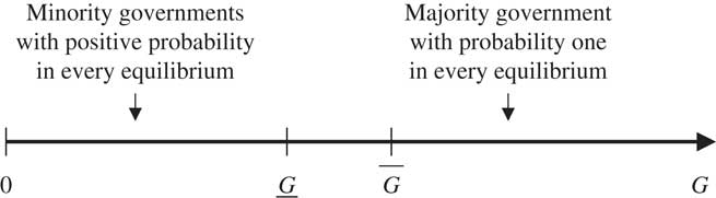
Fig. 1 Comparative statics
Note: since the bargaining game may admit multiple
equilibria, it is possible that in some intermediate range of cabinet
spoils
 $$(\underline{G} ,\overline{G} )$$
only a subset of equilibria involve minority
governments with positive probability.
$$(\underline{G} ,\overline{G} )$$
only a subset of equilibria involve minority
governments with positive probability.
In order to allow the reader to develop intuition for the reasons why we might expect such a result to hold, I now analyze an example. The configuration of party policy preferences in this example is a focal case in Baron (Reference Baron1991), and is assumed by Diermeier and Merlo (Reference Diermeier and Merlo2000) and Baron and Diermeier (Reference Baron and Diermeier2001). The example differs from the former study in that I explicitly introduce portfolio allocations, in addition to policies, as part of the government agreement, and from the latter two studies because I do not assume transferable utility.
Example 1: Let the space of policies be of dimension d=2. Assume n=3 parties with quadratic policy preferences given byFootnote 11
 $$U_{i} {\rm (}{\bf x}{\rm ,}\ {\bf g}{\rm )=}\,\tilde{u}_{i} {\rm (}{\bf x}{\rm )\,{+}}\,g_{i} {\rm \,=\,}K^{2} \,−\,\left( {x_{{\rm 1}} {\,−\,}\hat{x}_{{\rm 1}}^{i} } \right)^{2} −\,\left( {x_{{\rm 2}} {\,−\,}\hat{x}_{{\rm 2}}^{i} } \right)^{2} {\rm \,{+}}\,g_{i} {\rm ,}\,i\,{\rm=\!1,}\,{\rm 2,}\,{\rm 3}{\rm .}$$
Parties’ ideal policy points lie at the corners of an equilateral
triangle as shown in Figure 2a,
and are given by
 ${ \hat {\bf x}}^{1} {\rm =}\left( {{K \over 2},{{\sqrt 3 K} \over 2}} \right)$
,
${ \hat {\bf x}}^{1} {\rm =}\left( {{K \over 2},{{\sqrt 3 K} \over 2}} \right)$
,
 $${ \hat {\bf x}}^{2} {\rm =}(0,0)$$
, and
$${ \hat {\bf x}}^{2} {\rm =}(0,0)$$
, and
 $${ \hat {\bf x}}^{3} {\rm =}({\rm 0},K)$$
, for some constant K>0.
Probabilities of recognition and discount factors are given by
$${ \hat {\bf x}}^{3} {\rm =}({\rm 0},K)$$
, for some constant K>0.
Probabilities of recognition and discount factors are given by
 $p_{i} {\rm \,>\, }{\textstyle{{\rm 1} \over {\rm 3}}}$
and δ
i
=δ for every party i,
respectively. There exists a pure strategy equilibrium in this game,Footnote
12
which is displayed in Figure
2a, such that proposing party 1 coalesces with party 2, party 2
with party 3, and party 3 with party 1. The equilibrium policy proposal
y
i
offered by party i coalescing with party
j is given by
$p_{i} {\rm \,>\, }{\textstyle{{\rm 1} \over {\rm 3}}}$
and δ
i
=δ for every party i,
respectively. There exists a pure strategy equilibrium in this game,Footnote
12
which is displayed in Figure
2a, such that proposing party 1 coalesces with party 2, party 2
with party 3, and party 3 with party 1. The equilibrium policy proposal
y
i
offered by party i coalescing with party
j is given by
 $${\bf x}^{{\{ i,j\} }} {\rm =}\,{\bf y}^{i} {\rm \,=}\,{\textstyle{{\rm 1} \over {\rm 2}}}{ \hat {\bf x}}^{i} {\rm \,{+}}\,{\textstyle{{\rm 1} \over {\rm 2}}}{ \hat {\bf x}}^{j} ,$$
when
 $G\geq \tilde{G}{\rm =}{{K^{2} ({\rm 9}-{\rm 7}\delta )} \over {{\rm 4}\delta }}$
, while it is a policy closer to the ideal point of
party i when
$G\geq \tilde{G}{\rm =}{{K^{2} ({\rm 9}-{\rm 7}\delta )} \over {{\rm 4}\delta }}$
, while it is a policy closer to the ideal point of
party i when
 $G{\rm \,<\, }\tilde{G}$
. Minority governments such that proposing party
i sets g
i
=G form with probability one when
$G{\rm \,<\, }\tilde{G}$
. Minority governments such that proposing party
i sets g
i
=G form with probability one when
 $$G\leq \tilde{G}$$
. Majority governments form with probability one when
$$G\leq \tilde{G}$$
. Majority governments form with probability one when
 $G{\rm \,>\, }\tilde{G}$
.
$G{\rm \,>\, }\tilde{G}$
.
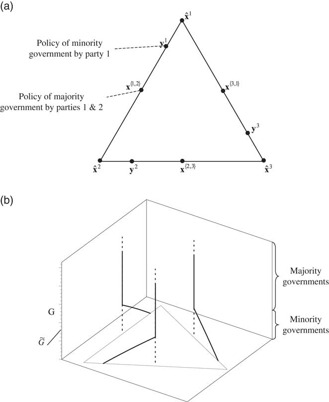
Fig. 2 Minority and majority governments in Example 1 (a) The (unconstrained)
ideal policies of the three parties are located at the vertices of the
equilateral triangle. The highlighted points are different policies
proposed in equilibrium for different values of parameter
G (b) For G below
 $$\tilde{G}$$
, minority governments form and policies are
leveraged toward the ideal point of the formateur. For
G above that level, only majority governments form
with policies at the midpoint between the ideal points of the two
parties in government.
$$\tilde{G}$$
, minority governments form and policies are
leveraged toward the ideal point of the formateur. For
G above that level, only majority governments form
with policies at the midpoint between the ideal points of the two
parties in government.
Example 1 exactly replicates the comparative statics illustrated in Figure 1. When policy polarization is
significant (low
 $$G\leq \tilde{G}$$
), minority governments form (in fact with probability one),
while only majority governments form when
$$G\leq \tilde{G}$$
), minority governments form (in fact with probability one),
while only majority governments form when
 $G{\rm \,>\, }\tilde{G}$
. Figure 2b displays
the change in equilibrium policy compromises as a function of the parameter
G. In order to illustrate the nature of the dependence of
the equilibrium outcome on parameters in Example 1, I now consider (without
loss of generality) the calculus of parties 1 and 2, with party 1 being the
formateur party. Party 1 wishes to propose a government that maximizes its
utility and obtains the support of party 2. Keeping with the notation in the
example, I denote by y
1, y
2, and y
3 the policies that prevail in equilibrium. Then, by rejecting a
proposal from party 1, party 2 expects to receive:
$G{\rm \,>\, }\tilde{G}$
. Figure 2b displays
the change in equilibrium policy compromises as a function of the parameter
G. In order to illustrate the nature of the dependence of
the equilibrium outcome on parameters in Example 1, I now consider (without
loss of generality) the calculus of parties 1 and 2, with party 1 being the
formateur party. Party 1 wishes to propose a government that maximizes its
utility and obtains the support of party 2. Keeping with the notation in the
example, I denote by y
1, y
2, and y
3 the policies that prevail in equilibrium. Then, by rejecting a
proposal from party 1, party 2 expects to receive:
 $${\textstyle{1 \over 3}}\tilde{u}_{2} {\rm (}{\bf y}^{1} {\rm )\,{+}}\,{\textstyle{1 \over 3}}\tilde{u}_{2} {\rm (}{\bf y}^{2} {\rm )\,{+}}\,{\textstyle{{\rm 1} \over {\rm 3}}}\tilde{u}_{2} {\rm (}{\bf y}^{3} {\rm )\,{+}}\,{\textstyle{G \over 3}}{\rm ,}$$
one period later. Here I make use of the symmetry of the
equilibrium in order to infer that, in expectation, party 2 receives one-third
of the cabinets,
 ${\textstyle{G \over {\rm 3}}}$
, in the next period.
${\textstyle{G \over {\rm 3}}}$
, in the next period.
Now suppose that there exists an equilibrium in which majority governments prevail with probability one. From Lemma 1 in the previous section, y i =x {i,j} , where policies x {i,j} maximize (3) for a majority government coalition by parties i and j, and are depicted graphically in Figure 2a.Footnote 13 Using the expression in (4) we deduce a contradiction to our hypothesis that majority governments form when:
 $$\tilde{u}_{2} \left( {{\bf x}^{{\left\{ {1,2} \right\}}} } \right)\geq \delta \left( {{\textstyle{1 \over 3}}\tilde{u}_{2} \left( {{\bf x}^{{\left\{ {1,2} \right\}}} } \right){\rm {\,+\,}}{\textstyle{1 \over 3}}\tilde{u}_{2} \left( {{\bf x}^{{\left\{ {2,3} \right\}}} } \right){\rm {\,+\,}}{\textstyle{1 \over 3}}\tilde{u}_{2} \left( {{\bf x}^{{\left\{ {3,1} \right\}}} } \right){\rm {\,+\,}}{\textstyle{G \over 3}}} \right){\rm ,}$$
since in this case party 2 is willing to approve a policy at x {1,2} without receiving any cabinets. A substantive interpretation of condition (5) is most clearly obtained by setting δ=1, whence inequality (5) is equivalent to
 $$\tilde{u}_{{\rm 2}} \left( {{\bf x}^{{\left\{ {1,2} \right\}}} } \right)\,−\,\tilde{u}_{2} \left( {{\bf x}^{{\left\{ {3,1} \right\}}} } \right)\geq G{\rm .}$$
If the policy preferences of political parties (hence the location of compromises x {i,j} ) are fixed, then the above condition is met when G is small. But another interpretation is that, for given G, condition (6) is satisfied when the policy of a majority government in which party 2 does not participate, x {3,1}, is distant (in utility terms) to the corresponding policy in a majority government this party participates, x {1,2}: in that case, party 2 is willing to accept a minority government with a policy at x {1,2} without receiving any cabinets, because otherwise it faces the risk of a policy at x {1,3} implemented by a coalition of parties 1 and 3 in the next period. Another perspective at the latter interpretation of condition (6) (that minority governments emerge in the presence of significant policy disagreement) is possible by considering what happens in Example 1 when parties’ ideal points all coincide (i.e., when K=0). Then compromises x {i,j} also coincide, and condition (6) fails for all G>0: all equilibrium governments are majority governments in the absence of political disagreement.
Assuming some political disagreement, as I do in the model, the challenge is to show that the above mechanism operates in more general bargaining environments. It turns out, as I show in the next example, that we cannot rule out the possibility of knife-edge configurations of model parameters for which the desired comparative static is not valid, because an inequality analogous to (5) fails for all G.
Example 2: (Counterexample) Let the space of policies be of dimension
d=2 and set X to be a square with
corners at
 $${\rm (0,}\ {\textstyle{{\rm 1} \over {\rm 3}}}{\rm )}$$
,
$${\rm (0,}\ {\textstyle{{\rm 1} \over {\rm 3}}}{\rm )}$$
,
 $${\rm (}{\textstyle{{\rm 1} \over {\rm 3}}}{\rm ,0)}$$
,
$${\rm (}{\textstyle{{\rm 1} \over {\rm 3}}}{\rm ,0)}$$
,
 ${\rm (0,−\,}{\textstyle{{\rm 1} \over {\rm 3}}}{\rm )}$
, and
${\rm (0,−\,}{\textstyle{{\rm 1} \over {\rm 3}}}{\rm )}$
, and
 $${\rm (−\,}{\textstyle{{\rm 1} \over {\rm 3}}}{\rm ,0)}$$
. Assume n=4 parties with equal share
of seats in parliament
$${\rm (−\,}{\textstyle{{\rm 1} \over {\rm 3}}}{\rm ,0)}$$
. Assume n=4 parties with equal share
of seats in parliament
 $$s_{i} \,{\rm =}\,{\textstyle{{\rm 1} \over {\rm 4}}}$$
, i=1, … , 4 and preferences given
by
$$s_{i} \,{\rm =}\,{\textstyle{{\rm 1} \over {\rm 4}}}$$
, i=1, … , 4 and preferences given
by
 $$U_{i} \left( {{\bf x},{\bf g}} \right)\,{\rm =}\,{\textstyle{{\rm 9} \over {{\rm 10}}}}\,−\,\left( {x_{1} \,−\,\hat{x}_{1}^{i} } \right)^{2} −\,{\textstyle{{\rm 1} \over {\rm 2}}}\left( {x_{2} \,−\,\hat{x}_{2}^{i} } \right)^{2} {\rm {+}}\,g_{i} {\rm ,}\,i\,{\rm =}\,{\rm 1,4,}$$
and
 $$U_{i} \left( {{\bf x},{\bf g}} \right){\rm \,=}\,{\textstyle{{\rm 9} \over {{\rm 10}}}}\,−\,{\textstyle{1 \over 2}}\left( {x_{1} \,−\,\hat{x}_{1}^{i} } \right)^{2} \,−\,\left( {x_{2} \,−\,\hat{x}_{2}^{i} } \right)^{2} {\rm {+}}\,g_{i} {\rm ,}\,i\,\,{\rm =}\,\,{\rm 2,4,}$$
where
 $${ \hat {\bf x}}^{{\rm 1}} \,{\rm =}\,\left( {{\rm 0,1}} \right)$$
,
$${ \hat {\bf x}}^{{\rm 1}} \,{\rm =}\,\left( {{\rm 0,1}} \right)$$
,
 $${ \hat {\bf x}}^{{\rm 2}} \,{\rm =}\,\left( {{\rm 1,0}} \right)$$
,
$${ \hat {\bf x}}^{{\rm 2}} \,{\rm =}\,\left( {{\rm 1,0}} \right)$$
,
 ${ \hat {\bf x}}^{{\rm 3}} \,\,{\rm =}\,\,\left( {{\rm 0,}−{\rm 1}} \right)$
, and
${ \hat {\bf x}}^{{\rm 3}} \,\,{\rm =}\,\,\left( {{\rm 0,}−{\rm 1}} \right)$
, and
 $${ \hat {\bf x}}^{{\rm 4}} \,{\rm =}\,\left( {−{\rm 1,0}} \right)$$
. Probabilities of recognition and discount factors are
identical and given by
$${ \hat {\bf x}}^{{\rm 4}} \,{\rm =}\,\left( {−{\rm 1,0}} \right)$$
. Probabilities of recognition and discount factors are
identical and given by
 $p_{i} \,{\rm =}\,{\textstyle{{\rm 1} \over {\rm 4}}}$
and
$p_{i} \,{\rm =}\,{\textstyle{{\rm 1} \over {\rm 4}}}$
and
 $\delta _{i} \,{\rm =}\,{\textstyle{{{\rm 36}} \over {{\rm 37}}}}$
for all i∈N,
respectively. For every level of G>0 there exists an
equilibrium such that party 1 proposes
$\delta _{i} \,{\rm =}\,{\textstyle{{{\rm 36}} \over {{\rm 37}}}}$
for all i∈N,
respectively. For every level of G>0 there exists an
equilibrium such that party 1 proposes
 $${\bf x}=\left( {0,{\textstyle{1 \over 5}}} \right)$$
and
$${\bf x}=\left( {0,{\textstyle{1 \over 5}}} \right)$$
and
 $${\bf g}\,{\rm =}\,\left( {{\textstyle{{{\rm (2}\,−\,\delta {\rm )}G} \over {\rm 2}}}{\rm ,}{\textstyle{{\delta G} \over {\rm 4}}}{\rm ,0,}{\textstyle{{\delta G} \over {\rm 4}}}} \right)$$
, party 2 proposes
$${\bf g}\,{\rm =}\,\left( {{\textstyle{{{\rm (2}\,−\,\delta {\rm )}G} \over {\rm 2}}}{\rm ,}{\textstyle{{\delta G} \over {\rm 4}}}{\rm ,0,}{\textstyle{{\delta G} \over {\rm 4}}}} \right)$$
, party 2 proposes
 $${\bf x}=\left( {{\textstyle{1 \over 5}},0} \right)$$
and
$${\bf x}=\left( {{\textstyle{1 \over 5}},0} \right)$$
and
 $${\bf g}\,{\rm =}\,\left( {{\textstyle{{\delta G} \over {\rm 4}}}{\rm ,}{\textstyle{{{\rm (2}\,−\,\delta {\rm )}G} \over {\rm 2}}}{\rm ,}{\textstyle{{\delta G} \over {\rm 4}}}{\rm ,0}} \right)$$
, party 3 proposes
$${\bf g}\,{\rm =}\,\left( {{\textstyle{{\delta G} \over {\rm 4}}}{\rm ,}{\textstyle{{{\rm (2}\,−\,\delta {\rm )}G} \over {\rm 2}}}{\rm ,}{\textstyle{{\delta G} \over {\rm 4}}}{\rm ,0}} \right)$$
, party 3 proposes
 $${\bf x}\,{\rm =}\,\left( {{\rm 0,}−{\textstyle{{\rm 1} \over {\rm 5}}}} \right)$$
and
$${\bf x}\,{\rm =}\,\left( {{\rm 0,}−{\textstyle{{\rm 1} \over {\rm 5}}}} \right)$$
and
 $${\bf g}=\left( {0,{\textstyle{{\delta G} \over 4}},{\textstyle{{(2{\,−\,}\delta )G} \over 2}},{\textstyle{{\delta G} \over 4}}} \right)$$
, and party 4 proposes
$${\bf g}=\left( {0,{\textstyle{{\delta G} \over 4}},{\textstyle{{(2{\,−\,}\delta )G} \over 2}},{\textstyle{{\delta G} \over 4}}} \right)$$
, and party 4 proposes
 ${\bf x}\,{\rm =}\,\left( {−{\textstyle{{\rm 1} \over {\rm 5}}}{\rm ,0}} \right)$
and
${\bf x}\,{\rm =}\,\left( {−{\textstyle{{\rm 1} \over {\rm 5}}}{\rm ,0}} \right)$
and
 $${\bf g}\,{\rm =}\,\left( {{\textstyle{{\delta G} \over {\rm 4}}}{\rm ,0,}{\textstyle{{\delta G} \over {\rm 4}}}{\rm ,}{\textstyle{{{\rm (2}\,−\,{\rm \delta )}G} \over {\rm 2}}}} \right)$$
.
$${\bf g}\,{\rm =}\,\left( {{\textstyle{{\delta G} \over {\rm 4}}}{\rm ,0,}{\textstyle{{\delta G} \over {\rm 4}}}{\rm ,}{\textstyle{{{\rm (2}\,−\,{\rm \delta )}G} \over {\rm 2}}}} \right)$$
.
It would appear that any intuition built using Example 1 is destroyed in view of Example 2. Counterexamples are typically fatal for the kind of general theory I wish to establish. What rescues the advertized theory of minority governments is the fact that I am able to show that such counterexamples are singularities. In particular, by using certain continuity results established by Banks and Duggan (Reference Banks and Duggan2000) and Kalandrakis (Reference Kalandrakis2006), it is possible to establish that the mechanism illustrated by Example 1 operates for almost all parameters (i.e., outside a set of zero Lebesgue measure). I state this result in the next Theorem.
Theorem 2: Fix utility functions u
i
, seat shares s
i
, and recognition probabilities p
i
and assume (M2). For almost all discount factors
δ
i
, and for almost all preference parameters c
i
, there exists
 $$\underline{G} $$
with
$$\underline{G} $$
with
 $\underline{G} {\rm \,> \!0}$
such that for all
$\underline{G} {\rm \,> \!0}$
such that for all
 $$G{\rm \,<\, }\underline{G} $$
, minority governments form with positive probability in
all equilibria of the corresponding government formation game.
$$G{\rm \,<\, }\underline{G} $$
, minority governments form with positive probability in
all equilibria of the corresponding government formation game.
Before I conclude this section, I take some time to further clarify the implications of Theorem 2 and discuss empirical evidence. A first remark is that Theorem 2 only ensures that in every equilibrium, minority governments occur with positive probability, not necessarily with probability one. This is fortunate, as it allows for the possibility of political systems in which both minority and majority governments occur with positive probability over time in the same equilibrium. Minority governments may occur with probability one in an equilibrium, as in the equilibrium of Example 1, but this is not always the case.
It is also tempting to interpret Theorems 1 and 2 as jointly implying that minority governments occur only when cabinet office is not significant and, hence, discount the importance of these results on the grounds that they are too intuitive. If “intuitive” in this context means a result that is obviously true, then this objection has already been addressed: as shown in Example 2, a naive statement of Theorem 2 has a counterexample, and statements that have counterexamples cannot be “obviously true.”
Furthermore, the above interpretation of Theorems 1 and 2 (that minority
governments occur only when cabinet posts are insignificant) is incorrect, at
least with empirically plausible quantifications of the relative significance
of cabinet office and policy. This is clear in the context of Example 1: set
K=1 and note that for discount factor
 $\delta \,{\rm =}\,{\textstyle{{\rm 9} \over {{\rm 10}}}}$
the value of
$\delta \,{\rm =}\,{\textstyle{{\rm 9} \over {{\rm 10}}}}$
the value of
 $$\underline{G} $$
is
$$\underline{G} $$
is
 $$\underline{G} =\tilde{G}=1$$
. That means party 1 values cabinets so much that it is
willing to implement the ideal policy of another party in order to get all
cabinets, instead of implementing its own ideal policy without cabinets. For a
smaller discount factor,
$$\underline{G} =\tilde{G}=1$$
. That means party 1 values cabinets so much that it is
willing to implement the ideal policy of another party in order to get all
cabinets, instead of implementing its own ideal policy without cabinets. For a
smaller discount factor,
 $\delta \,{\rm =}\,{\textstyle{{\rm 3} \over {\rm 5}}}$
,
$\delta \,{\rm =}\,{\textstyle{{\rm 3} \over {\rm 5}}}$
,
 $$\underline{G} =2$$
so that parties value holding cabinet office twice as much as
moving policy from the ideal of their worst ideological opponent to their own
ideal point. Although such trades may appear desirable for some individual
politicians within parties, they seem highly implausible when it comes to
partisan preferences. Yet, in Example 1 minority governments emerge with
probability one for any
$$\underline{G} =2$$
so that parties value holding cabinet office twice as much as
moving policy from the ideal of their worst ideological opponent to their own
ideal point. Although such trades may appear desirable for some individual
politicians within parties, they seem highly implausible when it comes to
partisan preferences. Yet, in Example 1 minority governments emerge with
probability one for any
 $G{\rm \,<\, }\tilde{G}$
under either pair of parameter specifications, that is, even
though parties value cabinet office disproportionally relative to policy.
$G{\rm \,<\, }\tilde{G}$
under either pair of parameter specifications, that is, even
though parties value cabinet office disproportionally relative to policy.
Furthermore, when attempting to interpret the empirical variation in the
incidence of minority governments across countries in light of Theorems 1 and
2, it is actually possible to fix the absolute value of cabinet office to a
common, arbitrarily high value. According to Theorem 2, at least some
equilibrium governments are guaranteed to be minority governments in countries
in which the ideological distance between the policy compromises pursued by
different coalitions is high. In the context of Example 1 this becomes obvious
by increasing the difference
 $\tilde{u}_{{\rm 2}} \left( {{\bf x}^{{\left\{ {{\rm 1,2}} \right\}}} } \right)\,−\,\tilde{u}_{{\rm 2}} \left( {{\bf x}^{{\left\{ {{\rm 3,1}} \right\}}} } \right)$
in inequality (6). Finally, note that in the model parties’
utility always increases with higher cabinet allocations, consistent with
requirement (b) in the introduction.
$\tilde{u}_{{\rm 2}} \left( {{\bf x}^{{\left\{ {{\rm 1,2}} \right\}}} } \right)\,−\,\tilde{u}_{{\rm 2}} \left( {{\bf x}^{{\left\{ {{\rm 3,1}} \right\}}} } \right)$
in inequality (6). Finally, note that in the model parties’
utility always increases with higher cabinet allocations, consistent with
requirement (b) in the introduction.
Intuitive or not, Theorems 1 and 2 are statements that are testable, and the pertinent question is whether the theory put forth by these theorems is corroborated by the data or not. Do we observe more minority governments as parties get more ideologically polarized or as cabinet office becomes relatively less important as a source of party payoffs? A number of scholars have provided evidence that is consistent with these predictions. For example, Indridason (Reference Indridason2005) attributes the higher incidence of majority governments in Iceland compared with other Scandinavian countries to the higher importance of cabinet office owing to the prevalence of clientelism practices. Furthermore, Sened (Reference Sened1996), using data from Israel shows how the emergence of minority governments there is related to the polarization of the party system. Finally, in a “large n” study, Warwick (Reference Warwick1998) shows that minority governments are more likely to form when policy polarization increases or when cabinet office becomes more important, respectively.
Conclusions
I have derived a theory for the emergence of minority and majority governments in multiparty parliamentary systems using a sequential bargaining model. I established a comparative static to the effect that minority governments are (for almost all parameters) guaranteed to emerge with positive probability when policy disagreement or polarization is significant, or when utility from cabinet posts is relatively small compared with partisan policy disagreement. Majority governments form when these conditions are reversed. Throughout the analysis I maintained that cabinet office is valuable per se, and I avoided dimensionality or other ad hoc restrictions on the government agreements space. These findings are corroborated by a number of independent empirical studies.

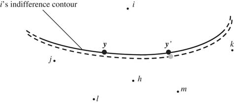
Fig. 3 Graphic illustration of Lemma 2
Note: policy y represents the solution to Equation 2 for coalition C={i,j,l,h}, while policy y ' represents the respective policy for coalition C={i,m,k}. For almost all preference parameters (c r ) r∈C∪C′, the two policies y and y ' do not fall on the same indifference contour of party i∈C∩C′.
Appendix
In the Appendix I prove all the numbered results that appear in the main
body of the paper. Before I start, I introduce some necessary notation. I
denote the set of portfolio allocations given parameter G
by
 ${\bf G}_{G} \,{\rm =\{ }{\bf g}\,\in\, {\Bbb R}_{{+}}^{n} {\rm :}\mathop{\sum}\nolimits_{i\,\in\, N} {g_{i} \,{\rm =}\,G} {\rm \} }$
. I also use v
i
to indicate the continuation value of party i in an
equilibrium, that is, the expected utility of this party if the proposal in
the current round is rejected.
${\bf G}_{G} \,{\rm =\{ }{\bf g}\,\in\, {\Bbb R}_{{+}}^{n} {\rm :}\mathop{\sum}\nolimits_{i\,\in\, N} {g_{i} \,{\rm =}\,G} {\rm \} }$
. I also use v
i
to indicate the continuation value of party i in an
equilibrium, that is, the expected utility of this party if the proposal in
the current round is rejected.
Theorem 1: (Restated) Fix utility functions u
i
, preference parameters c
i
, seat shares s
i
, recognition probabilities p
i
, and discount factors δ
i
and assume (M1). There exists
 $\overline{G} $
such that for every
$\overline{G} $
such that for every
 $G{\rm \,>\, }\overline{G} $
, all governments that form with positive probability
are majority governments in all equilibria of the corresponding
government formation game.
$G{\rm \,>\, }\overline{G} $
, all governments that form with positive probability
are majority governments in all equilibria of the corresponding
government formation game.
Proof. Define
 $$\overline{u} _{i} ={\rm max } \left\{ {u_{i} ({\bf x},0):{\bf x}\,\in\, X} \right\}$$
. I first claim that:
$$\overline{u} _{i} ={\rm max } \left\{ {u_{i} ({\bf x},0):{\bf x}\,\in\, X} \right\}$$
. I first claim that:
(1) Consider an equilibrium with discounted continuation values that
satisfy
 $\delta _{i} v_{i} {\rm \,>\, }\bar{u}_{i} $
for every non-dummy party i. All governments that form in that
equilibrium are majority governments. Suppose not. Then there
exists equilibrium proposal (y,
g)∈X×G
G
, a winning coalition C that approve government
(y, g), and a non-dummy party
j∈C such that g
j
=0. Then
$\delta _{i} v_{i} {\rm \,>\, }\bar{u}_{i} $
for every non-dummy party i. All governments that form in that
equilibrium are majority governments. Suppose not. Then there
exists equilibrium proposal (y,
g)∈X×G
G
, a winning coalition C that approve government
(y, g), and a non-dummy party
j∈C such that g
j
=0. Then
 $$U_{j} \left( {{\bf y},{\bf g};c_{j} } \right)=u_{j} \left( {{\bf y},0} \right)\geq \delta _{j} v_{j} \,>\, \overline{u} _{j} $$
, a contradiction.
$$U_{j} \left( {{\bf y},{\bf g};c_{j} } \right)=u_{j} \left( {{\bf y},0} \right)\geq \delta _{j} v_{j} \,>\, \overline{u} _{j} $$
, a contradiction.
Next I show that:
(2) For each party i with p
i
>0, there exists
 $$\overline{G} _{i} $$
such that
$$\overline{G} _{i} $$
such that
 $G{\rm \,>\, }\bar{G}_{i} \Rightarrow\delta _{i} v_{i} {\rm \,>\, }\bar{u}_{i} $
in every equilibrium. Fix some player i
and let
$G{\rm \,>\, }\bar{G}_{i} \Rightarrow\delta _{i} v_{i} {\rm \,>\, }\bar{u}_{i} $
in every equilibrium. Fix some player i
and let
 $\underline{u} _{i} {\rm =min}\left\{ {u_{i} ({\bf x},0){\rm :}{\bf x}\,\in\, X} \right\}$
. If
$\underline{u} _{i} {\rm =min}\left\{ {u_{i} ({\bf x},0){\rm :}{\bf x}\,\in\, X} \right\}$
. If
 $$\left( {\overline{{\bf y}} ,\overline{{\bf g}} } \right)$$
is the expected value of proposals in an SSP equilibrium,
then
$$\left( {\overline{{\bf y}} ,\overline{{\bf g}} } \right)$$
is the expected value of proposals in an SSP equilibrium,
then
 $$\left( {\overline{{\bf y}} ,\overline{{\bf g}} } \right)\,\in\, X{\times}{\bf G}_{G} $$
owing to the convexity of
X×G
G
and we have
$$\left( {\overline{{\bf y}} ,\overline{{\bf g}} } \right)\,\in\, X{\times}{\bf G}_{G} $$
owing to the convexity of
X×G
G
and we have
 $$\delta _{j} v_{j} \leq U_{j} \left( {\overline{{\bf y}} ,\overline{{\bf g}} ;c_{j} } \right)$$
, for all j∈N, owing to
the concavity of u
j
. For government
$$\delta _{j} v_{j} \leq U_{j} \left( {\overline{{\bf y}} ,\overline{{\bf g}} ;c_{j} } \right)$$
, for all j∈N, owing to
the concavity of u
j
. For government
 $$\left( {\overline{{\bf y}} ,\overline{{\bf g}} } \right)$$
, let h≠i be such that
$$\left( {\overline{{\bf y}} ,\overline{{\bf g}} } \right)$$
, let h≠i be such that
 $$\overline{g} _{h} \geq \overline{g} _{j} $$
for all
j∈N\{i}, that is,
h is the party with the highest expected portfolio
allocation among parties other than i. Since
$$\overline{g} _{h} \geq \overline{g} _{j} $$
for all
j∈N\{i}, that is,
h is the party with the highest expected portfolio
allocation among parties other than i. Since
 $\bar{g}_{h} \geq {\textstyle{{G-\bar{g}_{i} } \over {n\,−\,1}}}$
we have
$\bar{g}_{h} \geq {\textstyle{{G-\bar{g}_{i} } \over {n\,−\,1}}}$
we have
 $\overline{g} _{i} {\rm {+}}\overline{g} _{h} \geq {\textstyle{G \over {n\,−\,{\rm 1}}}}$
. Thus, proposal
$\overline{g} _{i} {\rm {+}}\overline{g} _{h} \geq {\textstyle{G \over {n\,−\,{\rm 1}}}}$
. Thus, proposal
 $(\overline{{\bf y}} {\rm ,}\ {\bf g}^\prime)\,\in\, X{\times}{\bf G}_{G} $
with
$(\overline{{\bf y}} {\rm ,}\ {\bf g}^\prime)\,\in\, X{\times}{\bf G}_{G} $
with
 $$g'_{j} =\overline{g} _{j} $$
if j≠i,
h,
$$g'_{j} =\overline{g} _{j} $$
if j≠i,
h,
 $$g'_{h} =0$$
, and
$$g'_{h} =0$$
, and
 $g_{i}^{\prime} \,{\rm =}\,\bar{g}_{i} {\rm \,{+}\,}\bar{g}_{h} \geq {1 \over {n\,−\,1}}G$
is approved by all parties except party
h. Hence, party i can guarantee her party
a utility level
$g_{i}^{\prime} \,{\rm =}\,\bar{g}_{i} {\rm \,{+}\,}\bar{g}_{h} \geq {1 \over {n\,−\,1}}G$
is approved by all parties except party
h. Hence, party i can guarantee her party
a utility level
 $$U_{i} \left( {\overline{{\bf y}} ,{\bf g}';c_{i} } \right)$$
when proposing. Thus, i’s continuation
value must satisfy
$$U_{i} \left( {\overline{{\bf y}} ,{\bf g}';c_{i} } \right)$$
when proposing. Thus, i’s continuation
value must satisfy
 $v_{i} \geq \left( {1{\,−\,}p_{i} } \right)\underline{u} _{i} {\rm \,{+}\,}p_{i} \left( {u_{i} \left( {\overline{{\bf y}} ,{\textstyle{G \over {n{\,−\,}1}}}} \right){\rm \,{+}\,}c_{i} {\textstyle{G \over {n{\,−\,}1}}}} \right)$
. Note that
$v_{i} \geq \left( {1{\,−\,}p_{i} } \right)\underline{u} _{i} {\rm \,{+}\,}p_{i} \left( {u_{i} \left( {\overline{{\bf y}} ,{\textstyle{G \over {n{\,−\,}1}}}} \right){\rm \,{+}\,}c_{i} {\textstyle{G \over {n{\,−\,}1}}}} \right)$
. Note that
 $$u_{i} \left( {\overline{{\bf y}} ,0} \right)\geq \underline{u} _{i} $$
for all possible
$$u_{i} \left( {\overline{{\bf y}} ,0} \right)\geq \underline{u} _{i} $$
for all possible
 $$\overline{{\bf y}} \,\in\, X$$
. Since p
i
>0, δ
i
∈(0,1], c
i
>0, and
$$\overline{{\bf y}} \,\in\, X$$
. Since p
i
>0, δ
i
∈(0,1], c
i
>0, and
 $${{\partial u_{i} (\overline{{\bf y}} ,\ g_{i} )} \over {\partial g_{i} }}> 0$$
for all
$${{\partial u_{i} (\overline{{\bf y}} ,\ g_{i} )} \over {\partial g_{i} }}> 0$$
for all
 $$\overline{{\bf y}} \,\in\, X$$
, there exists
$$\overline{{\bf y}} \,\in\, X$$
, there exists
 $\overline{G} _{i} {\rm \,>\, 0}$
such that
$\overline{G} _{i} {\rm \,>\, 0}$
such that
 $$\delta _{i} \left( {\left( {1-p_{i} } \right)\underline{u} _{i} {\rm \,{+}\,}p_{i} \left( {u_{i} \left( {\overline{{\bf y}} ,{\textstyle{G \over {n\,−\,1}}}} \right){\rm \,{+}\,}c_{i} {\textstyle{G \over {n\,−\,1}}}} \right)} \right)> \overline{u} _{i} $$
for all
$$\delta _{i} \left( {\left( {1-p_{i} } \right)\underline{u} _{i} {\rm \,{+}\,}p_{i} \left( {u_{i} \left( {\overline{{\bf y}} ,{\textstyle{G \over {n\,−\,1}}}} \right){\rm \,{+}\,}c_{i} {\textstyle{G \over {n\,−\,1}}}} \right)} \right)> \overline{u} _{i} $$
for all
 $$G> \overline{G} _{i} $$
and all
$$G> \overline{G} _{i} $$
and all
 $$\overline{{\bf y}} \,\in\, X$$
. As a result,
$$\overline{{\bf y}} \,\in\, X$$
. As a result,
 $$G> \overline{G} _{i} \Rightarrow\delta _{i} v_{i} {\rm \,>\, }\overline{u} _{i} $$
, completing the proof of Step (2).
$$G> \overline{G} _{i} \Rightarrow\delta _{i} v_{i} {\rm \,>\, }\overline{u} _{i} $$
, completing the proof of Step (2).
Set
 $$\overline{G} =max\left\{ {\overline{G} _{i} \,\mid\,i\,{\rm with}\,p_{i} \,>\, 0} \right\}$$
. Now
$$\overline{G} =max\left\{ {\overline{G} _{i} \,\mid\,i\,{\rm with}\,p_{i} \,>\, 0} \right\}$$
. Now
 $$G{\rm \,>\, }\overline{G} \Rightarrow\delta _{i} v_{i} {\rm \,>\, }\overline{u} _{i} $$
for all i with p
i
>0, in every equilibrium by Step (2). But then only majority
governments form for
$$G{\rm \,>\, }\overline{G} \Rightarrow\delta _{i} v_{i} {\rm \,>\, }\overline{u} _{i} $$
for all i with p
i
>0, in every equilibrium by Step (2). But then only majority
governments form for
 $$G{\rm \,>\, }\overline{G} $$
in every equilibrium, by Step (1).□
$$G{\rm \,>\, }\overline{G} $$
in every equilibrium, by Step (1).□
Lemma 1: (Restated) Assume (M2). If a majority government (x, g) proposed by party i forms in equilibrium and the set of parties receiving cabinet portfolios is given by C, then i∈C, all parties j∈C, j≠i, are indifferent between accepting or rejecting (x, g), and the policy x maximizes
 $$\mathop{\sum}\limits_{j\,\in\, C} w_{j} u_{j} ({\bf y},g_{j} ){\rm ,}$$
over y∈X, holding the
portfolio allocation g and weights
 $$w_{j} =\left( {{{\partial u_{j} \left( {x,g_{i} } \right)} \over {\partial g_{i} }}{+}c_{j} } \right)^{{{−}1}} $$
fixed.
$$w_{j} =\left( {{{\partial u_{j} \left( {x,g_{i} } \right)} \over {\partial g_{i} }}{+}c_{j} } \right)^{{{−}1}} $$
fixed.
Proof. Let majority government (x, g) be proposed by party i in an equilibrium with continuation values v h , h∈N. First note that
 $$U_{j} \left( {{\bf x,g};c_{j} } \right)\,{\rm =}\,\delta _{j} v_{j} {\rm ,}\,{\rm for}\,{\rm all}\,j\,\in\, C\,\backslash\,\left\{ i \right\}{\rm ,}$$
which follows from the fact that
 $${{\partial u_{h} \left( {{\bf x},\ g_{h} } \right)} \over {\partial g_{h} }}\,{+}\,c_{h} \,>\, 0$$
,
$${{\partial u_{h} \left( {{\bf x},\ g_{h} } \right)} \over {\partial g_{h} }}\,{+}\,c_{h} \,>\, 0$$
,
 $${{\partial u_{h} \left( {{\bf x},\ g_{h} } \right)} \over {\partial g_{l} }}=0$$
for all x∈X,
l≠h, h,
l∈N. Specifically, if
U
j
(x, g; c
j
)>δ
j
v
j
, j∈C\{i}, then by
the continuity of U
j
(x, g; c
j
) it is possible to reduce g
j
and increase g
i
(and party i’s utility) with the new government
still being invested. Similarly, if U
j
(x, g; c
j
)<δ
j
v
j
, j∈C\{i} then it
is possible to set g
j
=0 and increase g
i
(and party i’s utility) with the new government
still being invested. Furthermore, the same arguments and the fact that, by
(M2), the proposing party i cannot be
redundant in any winning coalition in which no other party is redundant
ensure that i∈C, that is, the proposing
party is included among the parties receiving cabinets.
$${{\partial u_{h} \left( {{\bf x},\ g_{h} } \right)} \over {\partial g_{l} }}=0$$
for all x∈X,
l≠h, h,
l∈N. Specifically, if
U
j
(x, g; c
j
)>δ
j
v
j
, j∈C\{i}, then by
the continuity of U
j
(x, g; c
j
) it is possible to reduce g
j
and increase g
i
(and party i’s utility) with the new government
still being invested. Similarly, if U
j
(x, g; c
j
)<δ
j
v
j
, j∈C\{i} then it
is possible to set g
j
=0 and increase g
i
(and party i’s utility) with the new government
still being invested. Furthermore, the same arguments and the fact that, by
(M2), the proposing party i cannot be
redundant in any winning coalition in which no other party is redundant
ensure that i∈C, that is, the proposing
party is included among the parties receiving cabinets.
Now suppose x does not maximize the objective in (3). First I show that x must be at least a local maximizer of (3). If not, then we can change x in a feasible direction v such that
 $$\mathop{\sum}\limits_{j\,\in\, C} {\left( {{{\partial u_{j} ({\bf x},g_{j} )} \over {\partial g_{j} }}{\rm \,{+}\,}c_{j} } \right)^{{{−}1}} D_{{\bf x}} u_{j} ({\bf x},g_{j} ) \cdot {\bf v}\,{\rm =}\,d> 0.} $$
For n′=|C|, set
 $$d_{j} \,{\rm =}\,{d \over {n'}}\,−\,\left( {{{\partial u_{j} ({\bf x},g_{j} )} \over {\partial g_{j} }}{\rm \,{+}\,}c_{j} } \right)^{{{−}1}} D_{{\bf x}} u_{j} ({\bf x},g_{j} ) \cdot {\bf v},$$
for all j∈C, set d j =0 for all j∉C and note that ∑ j∈N d j =0. Thus, set a direction of change for g given by d=(d 1, … , d n ), and consider the effect that a change of (x, g) in the feasible direction (v, d) has on U j (x, g; c j ):
 $$D_{{({\bf x},\ {\bf g})}} U_{j} ({\bf x},{\bf g};c_{j} ) \cdot ({\bf v},{\bf d})\,{\rm =}\,D_{{\bf x}} u_{j} ({\bf x},g_{j} ) \cdot {\bf v}{\rm \,{+}}\left( {{{\partial u_{j} ({\bf x},g_{j} )} \over {\partial g_{j} }}{\rm \,{+}\,}c_{j} } \right)d_{j} \,{\rm =}\,\left( {{{\partial u_{j} ({\bf x},g_{j} )} \over {\partial g_{j} }}{\rm \,{+}\,}c_{j} } \right){d \over {n'}}> 0,$$
for all j∈C, which is a contradiction: government (x, g) cannot be optimal for formateur i∈C since there exists a feasible direction that improves all coalition partners’ payoff. Thus, x is a local maximizer of (3). Since the latter is strictly concave as the sum of strictly concave functions, x is also a global maximizer over alternatives in X.□
Before I prove Theorem 2 I will prove a second lemma, which I illustrate
using Figure 3. This figure displays
a two-dimensional policy space and the ideal policy points of members of two
winning coalitions with party i belonging in both
coalitions. The two highlighted policy points display the policies that
satisfy Equation 2 for
these two coalitions. The lemma establishes that for almost all parameters
 $$(c_{i} )_{{i\,\in\, N}} \,\in\, (0,\overline{c} )^{n} $$
these policies cannot lie on the same indifference contour
of players in the intersection of C and
C′:
$$(c_{i} )_{{i\,\in\, N}} \,\in\, (0,\overline{c} )^{n} $$
these policies cannot lie on the same indifference contour
of players in the intersection of C and
C′:
Lemma 2: Consider distinct majority coalitions C,
C′. Outside a measure zero set
 $${\cal C}(C,C')\,\subset\,(0,\overline{c} )^{n} $$
of parameters
$${\cal C}(C,C')\,\subset\,(0,\overline{c} )^{n} $$
of parameters
 $$(c_i)_{i\in N}$$
, if distinct policies y, y
' satisfy (2) for coalitions C and
C′, respectively, then equations
$$(c_i)_{i\in N}$$
, if distinct policies y, y
' satisfy (2) for coalitions C and
C′, respectively, then equations
 $$U_{j} ({\bf y},{\bf 0};c_{j} )=U_{j} ({\bf y'},{\bf 0};c_{j} ),\,{\rm for}\,{\rm all}\,j\,\in\, C\,{\cap}\,C',$$
are inconsistent.
Proof. Let
ν=|C∪C′|. By
assumption y, y′∈int(X).
Furthermore, since these policies are distinct, we have (y,
y′)∈(int(X)×int(X)−Δ),
where Δ is the diagonal of int(X)×int(X).
Set
 $$S\,{\rm =}\,\left( {{\mathop{\rm int}} (X){\times}{\mathop{\rm int}} (X) \,−\, \Delta } \right){\times}(0,\overline{c} )^{\nu } $$
and define |C∩C′|
functions
$$S\,{\rm =}\,\left( {{\mathop{\rm int}} (X){\times}{\mathop{\rm int}} (X) \,−\, \Delta } \right){\times}(0,\overline{c} )^{\nu } $$
and define |C∩C′|
functions
 $F_{j} {\rm \,:}\,S\to{\Bbb R}^{{2d{+}1}} $
,
j∈C∩C′, to be the
left-hand side of the following 2d+1
equations:
$F_{j} {\rm \,:}\,S\to{\Bbb R}^{{2d{+}1}} $
,
j∈C∩C′, to be the
left-hand side of the following 2d+1
equations:
 $$\matrix{ {\mathop{\sum}\limits_{h\,\in\, C} {\left( {m_{h} {\rm \,{+}\,}c_{h} } \right)^{{{−}1}} D_{{\bf y}} u_{h} \left( {{\bf y},0} \right)\,{\rm =}\,{\bf 0}} ,} \cr {\mathop{\sum}\limits_{h\,\in\, C'} {\left( {m_{h} {\rm \,{+}\,}c_{h} } \right)^{{{−}1}} D_{{{\bf y'}}} u_{h} \left( {{\bf y'},0} \right)\,{\rm =}\,{\bf 0},} } \cr {u_{j} \left( {{\bf y},0} \right){\rm −\,}u_{j} \left( {{\bf y'},0} \right)\,{\rm =}\,0.} \cr } $$
The first 2d equations represent Equation 2 for coalitions
C and C′, respectively. The domain of
each F
j
is the space of policies y, y′ and that of
the |C∪C′| parameters c
h
, h∈C∪C′, that is,
 $$S=\left( {{\mathop{\rm int}} (X){\times}{\mathop{\rm int}} (X){\,−\,}\Delta } \right){\times}(0,\overline{c} )^{\nu } $$
. Recall that z∈S is a
critical point of mapping F
j
if the Jacobian of F
j
evaluated at z, D
z
F
j
(z), does not have full rank. Consider the
set
$$S=\left( {{\mathop{\rm int}} (X){\times}{\mathop{\rm int}} (X){\,−\,}\Delta } \right){\times}(0,\overline{c} )^{\nu } $$
. Recall that z∈S is a
critical point of mapping F
j
if the Jacobian of F
j
evaluated at z, D
z
F
j
(z), does not have full rank. Consider the
set
 $$K_{j} \,{\rm =}\,\left\{ {{\bf z}\,\in\, F_{j}^{{{\,−\,}1}} ({\bf 0}):{\bf z}\ {\rm is}\,{\rm a}\,{\rm critical}\,{\rm point}\,{\rm of}\,F_{j} } \right\}.$$
I will first show:
 $$\bigcap\limits_{j\,\in\, C{\cap}C'} {K_{j} =\emptyset.} $$
Assume there exists z∈∩ j∈C∩C′ K j , instead, to get a contradiction. In what follows I index parties using the convention q∈C\C′, q′∈C′\C, and l∈(C∪C′−{j}). Calculating the Jacobian D z F j (z) using the order of variables implied by z=(y, y′, c j , c l , … , c q , … , c q′), we get:
 $$D_{{\bf z}} F_{j} ({\bf z})\,{\rm =}\,\left[ {\matrix{ A \hfill & {\bf 0} \hfill & {{−}w_{j}^{{{−}2}} {\bf a}_{j} } \hfill & {{−}w_{l}^{{{−}2}} {\bf a}_{l} } \hfill & \,\ldots\, \hfill & {{−}w_{q}^{{{−}2}} {\bf a}_{q} } \hfill & \,\ldots\, \hfill & {\bf 0} \hfill & \,\ldots\, \hfill \cr {\bf 0} \hfill & B \hfill & {{−}w_{j}^{{{−}2}} {\bf b}_{j} } \hfill & {{−}w_{l}^{{{−}2}} {\bf b}_{l} } \hfill & \,\ldots\, \hfill & {\bf 0} \hfill & \,\ldots\, \hfill & {{−}w_{{q'}}^{{{−}2}} {\bf b}_{{q'}} } \hfill & \,\ldots\, \hfill \cr {{\bf a}_{j}^{T} } \hfill & {{−}{\bf b}_{j}^{T} } \hfill & 0 \hfill & 0 \hfill & \,\ldots\, \hfill & 0 \hfill & \,\ldots\, \hfill & 0 \hfill & \,\ldots\, \hfill \cr } } \right],$$
where w
h
=m
h
+c
h
, h∈C∪C′,
 $$A\,{\rm =}\,\mathop{\sum}\nolimits_{h\,\in\, C} w_{h}^{{{−}1}} D_{{\bf y}}^{2} u_{h} \left( {{\bf y},0} \right)$$
,
$$A\,{\rm =}\,\mathop{\sum}\nolimits_{h\,\in\, C} w_{h}^{{{−}1}} D_{{\bf y}}^{2} u_{h} \left( {{\bf y},0} \right)$$
,
 $$B\,{\rm =}\,\mathop{\sum}\nolimits_{h\,\in\, C'} w_{h}^{{{\,−}1}} D_{{{\bf y'}}}^{2} u_{h} \left( {{\bf y'},0} \right)$$
, a
h
=D
y
u
h
(y, 0) and b
h
=D
y′
u
h
(y′, 0). Note that by assumption
w
h
>0, h∈C∪C′.
Performing a few equivalence operations on D
z
F
j
(z) we get a new matrix with the same rank:
$$B\,{\rm =}\,\mathop{\sum}\nolimits_{h\,\in\, C'} w_{h}^{{{\,−}1}} D_{{{\bf y'}}}^{2} u_{h} \left( {{\bf y'},0} \right)$$
, a
h
=D
y
u
h
(y, 0) and b
h
=D
y′
u
h
(y′, 0). Note that by assumption
w
h
>0, h∈C∪C′.
Performing a few equivalence operations on D
z
F
j
(z) we get a new matrix with the same rank:
 $$\left[ {\matrix{ A \hfill & {\bf 0} \hfill & {w_{j}^{{{−}1}} {\bf a}_{j} } \hfill & {w_{l}^{{{−}1}} {\bf a}_{l} } \hfill & \,\ldots\, \hfill & {w_{q}^{{{−}1}} {\bf a}_{q} } \hfill & \,\ldots\, \hfill & {\bf 0} \hfill & \,\ldots\, \hfill \cr {\bf 0} \hfill & B \hfill & {w_{j}^{{{−}1}} {\bf b}_{j} } \hfill & {w_{l}^{{{−}1}} {\bf b}_{l} } \hfill & \,\ldots\, \hfill & {\bf 0} \hfill & \,\ldots\, \hfill & {w_{{q'}}^{{{−}1}} {\bf b}_{{q'}} } \hfill & \,\ldots\, \hfill \cr {w_{j}^{{{−}1}} {\bf a}_{j}^{T} } \hfill & {{−}w_{j}^{{{−}1}} {\bf b}_{j}^{T} } \hfill & 0 \hfill & 0 \hfill & \,\ldots\, \hfill & 0 \hfill & \,\ldots\, \hfill & 0 \hfill & \,\ldots\, \hfill \cr } } \right].$$
Since A, B are negative definite, the above matrix has full rank if and only if the 1×m matrix:
 $$M_{j} ({\bf z})\,{\rm =}\,0{\rm \,−\,}\left[ {\matrix{ {w_{j}^{{{\rm \,−1}}} {\bf a}_{j} } \hfill \cr {{\rm \,−}w_{j}^{{{\rm \,−}1}} {\bf b}_{j} } \hfill \cr } } \right]^{T} \left[ {\matrix{ {A^{{{−}1}} } \hfill & 0 \hfill \cr 0 \hfill & {B^{{{−}1}} } \hfill \cr } } \right]\left[ {\matrix{ {w_{j}^{{{−}1}} {\bf a}_{j} } \hfill & {w_{l}^{{{−}1}} {\bf b}_{l} } \hfill & \,\ldots\, \hfill & {w_{q}^{{{−}1}} {\bf a}_{q} } \hfill & \,\ldots\, \hfill & {\bf 0} \hfill & \,\ldots\, \hfill \cr {w_{j}^{{{−}1}} {\bf b}_{j} } \hfill & {w_{l}^{{{−}1}} {\bf b}_{l} } \hfill & \,\ldots\, \hfill & {\bf 0} \hfill & \,\ldots\, \hfill & {w_{{q'}}^{{{−}1}} {\bf b}_{{q'}} } \hfill & \,\ldots\, \hfill \cr } } \right].$$
has rank 1. Since z∈∩
j∈C∩C′
K
j
, we have
 $${\bf z}\,\in\, F_{j}^{{−{\rm 1}}} (0)$$
for all j, so that y and
y′ satisfy Equation 2 and we obtain:
$${\bf z}\,\in\, F_{j}^{{−{\rm 1}}} (0)$$
for all j, so that y and
y′ satisfy Equation 2 and we obtain:
 $$\mathop{\sum}\limits_{h\,\in\, C} {w_{h}^{{{\,−}1}} {\bf a}_{h} } \,{\rm =}\,\,{\bf 0}\Rightarrow\mathop{\sum}\limits_{j\,\in\, C{\cap}C'} {w_{j}^{{{−}1}} {\bf a}_{j} } \,{\rm =}\,-\mathop{\sum}\limits_{q\,\in\, C\,\backslash\,C'} {w_{q}^{{{−}1}} {\bf a}_{q} {\rm ,}\,{\rm and}} $$
 $$\mathop{\sum}\limits_{k\,\in\, C'} {w_{h}^{{{−}1}} {\bf b}_{h} \,} \,{\rm =}\,\,{\bf 0}\Rightarrow\mathop{\sum}\limits_{j\,\in\, C{\cap}C'} {w_{j}^{{{−}1}} {\bf b}_{j} } \,{\rm =}\,-\mathop{\sum}\limits_{q'\,\in\, C'\,\backslash\,C} {w_{{q'}}^{{{−}1}} {\bf b}_{{q'}} .} $$
Furthermore, since z∈∩
j∈C∩C′
K
j
, z is a critical point of each F
j
, so we must have M
j
(z)=0 for all
j∈C∩C′.
M
j
(z)=0 means
 $$w_{j}^{{{−}1}} {\bf a}_{j}^{T} A^{{{−}1}} w_{q}^{{{−}1}} {\bf a}_{q} =0$$
for all
q∈C\C′ and all
j∈C∩C′, and we can
obtain (by summing equations
$$w_{j}^{{{−}1}} {\bf a}_{j}^{T} A^{{{−}1}} w_{q}^{{{−}1}} {\bf a}_{q} =0$$
for all
q∈C\C′ and all
j∈C∩C′, and we can
obtain (by summing equations
 $$w_{j}^{{{−}1}} {\bf a}_{j}^{T} A^{{{−}1}} w_{q}^{{{\,−}1}} {\bf a}_{q} \,{\rm =}\,0$$
first over all
q∈C\C′ for each
j∈C∩C′, and then over
all j):
$$w_{j}^{{{−}1}} {\bf a}_{j}^{T} A^{{{−}1}} w_{q}^{{{\,−}1}} {\bf a}_{q} \,{\rm =}\,0$$
first over all
q∈C\C′ for each
j∈C∩C′, and then over
all j):
 $$\left( {\mathop{\sum}\limits_{j\,\in\, C{\cap}C'} {w_{j}^{{{−}1}} {\bf a}_{j}^{T} } } \right)A^{{{−}1}} \left( {\mathop{\sum}\limits_{q\,\in\, C\,\backslash\,C'} w_{q}^{{{−}1}} {\bf a}_{q} } \right)\,{\rm =}\,0.$$
Using (A) and the fact that A −1 is negative definite, we deduce
 $$\mathop{\sum}\limits_{j\,\in\, C{\cap}C'} {w_{j}^{{{−}1}} {\bf a}_{j} } \,{\rm =}\,\mathop{\sum}\limits_{j\,\in\, C{\cap}C'} {\left( {m_{j} {\rm \,{+}\,}c_{j} } \right)^{{{−}1}} D_{{\bf y}} u_{j} \left( {{\bf y},0} \right)\,{\rm =}\,{\bf 0}.} $$
An identical argument using (B) gives us
 $$\mathop{\sum}\limits_{j\,\in\, C{\cap}C'} {w_{j}^{{{−}1}} {\bf b}_{j} } \,{\rm =}\,\mathop{\sum}\limits_{j\,\in\, C{\cap}C'} {(m_{j} {\rm \,{+}\,}c_{j} )^{{{−}1}} D_{{{\bf y'}}} u_{j} \left( {{\bf y'},0} \right)} \,{\rm =}\,{\bf 0}.$$
Since (C) and (D) imply that y , y ′ both maximize the strictly concave function ∑ j∈C∩C′(m j +c j )−1 u j (x, 0), we must have y=y′, which is impossible since z∈∩ j∈C∩C′ K j ⊂S. This completes the proof of (☆).
Now for each j∈C∩C′
define the map
 $$\hat{F}_{j} \,{\rm :}\,S\,\backslash\,K_{j} \to{\Bbb R}^{{2d{+}1}} $$
to be the restriction of F
j
on S\K
j
. Recall that
$$\hat{F}_{j} \,{\rm :}\,S\,\backslash\,K_{j} \to{\Bbb R}^{{2d{+}1}} $$
to be the restriction of F
j
on S\K
j
. Recall that
 $0\,\in\, {\Bbb R}^{{2d{\rm \,{+}\,}1}} $
is a regular value of
$0\,\in\, {\Bbb R}^{{2d{\rm \,{+}\,}1}} $
is a regular value of
 $$\hat{F}_{j} $$
if
$$\hat{F}_{j} $$
if
 $$D_{{\bf z}} \hat{F}_{j} ({\bf z})$$
has full rank for every
$$D_{{\bf z}} \hat{F}_{j} ({\bf z})$$
has full rank for every
 $${\bf z}\,\in\, \hat{F}_{j}^{{{\,−}1}} (0)$$
. Thus, since
$${\bf z}\,\in\, \hat{F}_{j}^{{{\,−}1}} (0)$$
. Thus, since
 $\hat{F}_{j}^{{{\,−}1}} (0)\,{\cap}\,K_{j} \,{\rm =}\, \emptyset $
by construction,
$\hat{F}_{j}^{{{\,−}1}} (0)\,{\cap}\,K_{j} \,{\rm =}\, \emptyset $
by construction,
 $$0\,\in\, {\Bbb R}^{{2d{+}1}} $$
is a regular value of
$$0\,\in\, {\Bbb R}^{{2d{+}1}} $$
is a regular value of
 $$\hat{F}_{j} $$
for all
j∈C∩C′. Note that
S is open and K
j
is a (relatively) closed set for all
j∈C∩C′, so that
S\K
j
is an open set for all
j∈C∩C′. Thus, each
$$\hat{F}_{j} $$
for all
j∈C∩C′. Note that
S is open and K
j
is a (relatively) closed set for all
j∈C∩C′, so that
S\K
j
is an open set for all
j∈C∩C′. Thus, each
 $$\hat{F}_{j} $$
is a smooth mapping between smooth manifolds since
S\K
j
is open and u
h
is smooth. As a result, the Preimage theorem (Guillemin and Pollack
Reference Guillemin and Pollack1974, 21) ensures that
$$\hat{F}_{j} $$
is a smooth mapping between smooth manifolds since
S\K
j
is open and u
h
is smooth. As a result, the Preimage theorem (Guillemin and Pollack
Reference Guillemin and Pollack1974, 21) ensures that
 $R_{j} \,{\rm =}\,\hat{F}_{j}^{{{\,−}1}} ({\bf 0})$
is at most a
(2d+ν)−(2d+1)=(ν−1)dimensional
manifold.
$R_{j} \,{\rm =}\,\hat{F}_{j}^{{{\,−}1}} ({\bf 0})$
is at most a
(2d+ν)−(2d+1)=(ν−1)dimensional
manifold.
I am now ready to conclude the proof of the Lemma. In order for
z∈S to satisfy F
j
(z)=0 for some
j∈C∩C′ we must have
z∈R
j
∪K
j
. It follows that in order for z∈S to
satisfy F
j
(z)=0 for all
j∈C∩C′, we must have
z∈∩
j∈C∩C′(R
j
∪K
j
). Since ∩
j∈C∩C′
K
j
=
 $\emptyset$
by (☆), the set ∩
j∈C∩C′(R
j
∪K
j
) can be rewritten as the finite union of sets that are themselves the
intersection of |C∩C′| sets, at least one
of which is at most a (ν−1) dimensional manifold. Thus, ∩
j∈C∩C′(R
j
∪K
j
) is itself at most (ν−1)-dimensional. This is one
dimension smaller than the space of parameters
$\emptyset$
by (☆), the set ∩
j∈C∩C′(R
j
∪K
j
) can be rewritten as the finite union of sets that are themselves the
intersection of |C∩C′| sets, at least one
of which is at most a (ν−1) dimensional manifold. Thus, ∩
j∈C∩C′(R
j
∪K
j
) is itself at most (ν−1)-dimensional. This is one
dimension smaller than the space of parameters
 $$\left( {c_{i} } \right)_{{i\,\in\, C{\cup}C'}} \,\in\, (0,\overline{c} )^{\nu } $$
and, as a consequence, the equations
$$\left( {c_{i} } \right)_{{i\,\in\, C{\cup}C'}} \,\in\, (0,\overline{c} )^{\nu } $$
and, as a consequence, the equations
 $$\matrix{ {\mathop{\sum}\limits_{h\,\in\, C} {\left( {m_{h} {\rm \,{+}\,}c_{h} } \right)^{{{\,−}1}} D_{{\bf y}} u_{h} \left( {{\bf y},0} \right)} \,{\rm =}\,{\bf 0},} \cr {\mathop{\sum}\limits_{h\,\in\, C'} {\left( {m_{h} {\rm \,{+}\,}c_{h} } \right)^{{{\,−}1}} D_{{{\bf y'}}} u_{h} \left( {{\bf y'},0} \right)\,{\rm =}\,{\bf 0},} } \cr {u_{j} \left( {{\bf y},0} \right)-u_{j} \left( {{\bf y'},0} \right)\,{\rm =}\,0,j\,\in\, C\,{\cap}\,C',} \cr } $$
are consistent only for a set of measure zero
 $${\cal C}(C,C')$$
of parameters c
h
, h∈N. Since U
j
(x, 0; c
j
)=u
j
(x, 0), the proof is complete.□
$${\cal C}(C,C')$$
of parameters c
h
, h∈N. Since U
j
(x, 0; c
j
)=u
j
(x, 0), the proof is complete.□
Theorem 2: (Restated) Fix utility functions u
i
, seat shares s
i
, and recognition probabilities p
i
and assume (M2). For almost all discount
factors δ
i
, and for almost all preference parameters c
i
, there exists
 $$\underline{G} $$
with
$$\underline{G} $$
with
 $$\underline{G} {\rm \,> 0}$$
such that for all
$$\underline{G} {\rm \,> 0}$$
such that for all
 $G{\rm \,<\, }\underline{G} $
, minority governments form with positive probability
in all equilibria of the corresponding government formation game.
$G{\rm \,<\, }\underline{G} $
, minority governments form with positive probability
in all equilibria of the corresponding government formation game.
Proof. Fix any p i , s i , u i satisfying the model’s assumptions. I break the proof into four steps:
(1) For all discount factors (δ
i
)
i∈N
outside a measure zero set
 $${\cal D}\,\subset\,\left( {0,1} \right]^{n} $$
, there is a finite number of pure strategy equilibria in the game
with G=0. These equilibria are independent of
$${\cal D}\,\subset\,\left( {0,1} \right]^{n} $$
, there is a finite number of pure strategy equilibria in the game
with G=0. These equilibria are independent of
 $$(c_{i} )_{{i\,\in\, N}} \,\in\, (0,\overline{c} )^{n} $$
. The game with G=0 satisfies condition
(A1) of Lemma 2 of Kalandrakis (Reference Kalandrakis2006, 318). Thus, the number of pure strategy
equilibria of this game is finite by theorems 3(i), p. 323 and theorem 5, p.
325 of Kalandrakis (Reference Kalandrakis2006), for
almost all discount factors. Clearly, parameters
$$(c_{i} )_{{i\,\in\, N}} \,\in\, (0,\overline{c} )^{n} $$
. The game with G=0 satisfies condition
(A1) of Lemma 2 of Kalandrakis (Reference Kalandrakis2006, 318). Thus, the number of pure strategy
equilibria of this game is finite by theorems 3(i), p. 323 and theorem 5, p.
325 of Kalandrakis (Reference Kalandrakis2006), for
almost all discount factors. Clearly, parameters
 $$(c_{i} )_{{i\,\in\, N}} \,\in\, (0,\overline{c} )^{n} $$
do not affect the equilibrium set of the game with
G=0. Thus, Step 1 is proved.
$$(c_{i} )_{{i\,\in\, N}} \,\in\, (0,\overline{c} )^{n} $$
do not affect the equilibrium set of the game with
G=0. Thus, Step 1 is proved.
In what follows, I will say that a sequence of equilibria e k , one for each version of the game with G=G k >0, is minority barring if all governments proposed in each equilibrium e k are majority governments. I first conclude:
(2) Consider a sequence G k →0 and an associated minority barring sequence of equilibria e k →e. e is an equilibrium of the game with G=0, and for every party i with p i >0, if i proposes policy y ∈X in equilibrium e, then y satisfies Equation 2 for some majority coalition C with i∈C. The fact that e is an equilibrium follows from the upper-hemicontinuity of the equilibrium correspondence (Banks and Duggan Reference Banks and Duggan2000, 81, theorem 3). Suppose party i proposes policy y∈X in equilibrium e. Since only majority governments form in every equilibrium e k , there exists a sequence of majority governments (y k , g k )→(y, 0) that are in the support of party i’s proposal strategy in equilibrium e k , and, going to a subsequence if necessary, a majority coalition C with i∈C, such that g h,k >0 for all h∈C and g h,k =0 for all h∉C. By Lemma 1, each proposal (y k , g k ) satisfies the first-order conditions for a maximum of the objective in (3) so that we deduce that y maximizes ∑ j∈C (m j +c j )−1 u j (y, 0) (a strictly concave function) at g=0. By assumption, there exists x in the interior of X such that
 $$\mathop{\sum}\limits_{j\,\in\, C} {\left( {m_{j} {\rm \,{+}\,}c_{j} } \right)^{{−1}} D_{{\bf x}} u_{j} ({\bf x},0){\rm ={\bf 0}}.} $$
Hence, x=y is the unique maximizer satisfying Equation 2.
For the next step, let
 $${\cal C}^{{\ast}} \,{\rm =}\,{\cup}_{{(C,C')}} {\cal C}(C,C')$$
be the finite union over all pairs of winning coalitions
(C,C′) of the sets
$${\cal C}^{{\ast}} \,{\rm =}\,{\cup}_{{(C,C')}} {\cal C}(C,C')$$
be the finite union over all pairs of winning coalitions
(C,C′) of the sets
 $${\cal C}(C,C')$$
identified in Lemma 2. Note that
$${\cal C}(C,C')$$
identified in Lemma 2. Note that
 $${\cal C}^{{\ast}} $$
has measure zero as the finite union of sets of measure
zero. I show:
$${\cal C}^{{\ast}} $$
has measure zero as the finite union of sets of measure
zero. I show:
(3) For all
 $$(c_{i} )_{{i\,\in\, N}}\, \notin\,{\cal C}^{{\ast}}$$
, and for any sequence G
k
→0 with an associated minority barring sequence of equilibria
e
k
→e, e is an equilibrium in pure strategies. Fix
parameters
$$(c_{i} )_{{i\,\in\, N}}\, \notin\,{\cal C}^{{\ast}}$$
, and for any sequence G
k
→0 with an associated minority barring sequence of equilibria
e
k
→e, e is an equilibrium in pure strategies. Fix
parameters
 $$(c_{i} )_{{i\,\in\, N}} \, \notin \, {\cal C}^{{\ast}} $$
and consider sequences G
k
→0 with an associated sequence of equilibria e
k
→e. By Step 1, e is an equilibrium.
Suppose equilibrium e is in mixed strategies so that two
distinct policies y, y′∈X lie in
the support of some party i’s proposal strategy with
p
i
>0. Then, since both y and y′ are played
with positive probability in equilibrium e, and by
analogous arguments as those used in the previous step, there exists a
subsequence of equilibria (still indexed by k),
e
k
→e, and corresponding sequences of majority
governments (y
k
, g
k
)→(y, 0), (y′
k
, g′
k
)→(y′,0), that are in the support of party
i’s proposal strategy in equilibrium e
k
, and distinct winning coalitions C and
C′,
i∈C∩C′, such that
g
h,k
>0 and g'
q,k
>0 if and only if h∈C,
q∈C′, and
$$(c_{i} )_{{i\,\in\, N}} \, \notin \, {\cal C}^{{\ast}} $$
and consider sequences G
k
→0 with an associated sequence of equilibria e
k
→e. By Step 1, e is an equilibrium.
Suppose equilibrium e is in mixed strategies so that two
distinct policies y, y′∈X lie in
the support of some party i’s proposal strategy with
p
i
>0. Then, since both y and y′ are played
with positive probability in equilibrium e, and by
analogous arguments as those used in the previous step, there exists a
subsequence of equilibria (still indexed by k),
e
k
→e, and corresponding sequences of majority
governments (y
k
, g
k
)→(y, 0), (y′
k
, g′
k
)→(y′,0), that are in the support of party
i’s proposal strategy in equilibrium e
k
, and distinct winning coalitions C and
C′,
i∈C∩C′, such that
g
h,k
>0 and g'
q,k
>0 if and only if h∈C,
q∈C′, and
 $$U_{j} ({\bf y}_{k} ,{\bf g}_{k} ;c_{j} )=U_{j} ({\bf y}'_{k} ,{\bf g}_{k} ;c_{j} ),\,{\rm for}\,{\rm all}\,j\,\in\, C\,{\cap}\,C',$$
for all k. The indifference of all players j∈C∩C′ follows from the fact that the proposer i mixes between proposals (y k , g k ),(y ' k , g ' k ) and leaves all cabinet recipient parties indifferent between its proposal and their continuation value in equilibrium e k (Equation 7 in the proof of Lemma 2). by continuity and Step 2, we deduce that proposals y , y' offered in the limit equilibrium e must satisfy
 $$\matrix{ {\mathop{\sum}\limits_{j\,\in\, C} {\left( {m_{j} {\rm \,{+}\,}c_{j} } \right)^{{{\,−\,}1}} D_{{\bf y}} u_{j} ({\bf y},0)} {\rm ={\bf 0}},} \cr {\mathop{\sum}\limits_{j\,\in\, C'} {\left( {m_{j} {\rm \,{+}\,}c_{j} } \right)^{{{\,−\,}1}} D_{{\bf y}} u_{j} ({\bf y}',0)} \,{\rm =}\,{\bf 0},} \cr {U_{j} ({\bf y},{\bf 0};c_{j} )\,{\rm =}\,U_{j} ({\bf y}',{\bf 0};c_{j} ),\,{\rm for}\,{\rm all}\,j\,\in\, C\,{\cap}\,C'.} \cr } $$
Lemma 2 guarantees this is impossible outside the measure zero set
 $${\cal C}(C,C')$$
. Thus, since we have fix parameters
$${\cal C}(C,C')$$
. Thus, since we have fix parameters
 $(c_{i} )_{{i\,\in\, N}} \,\notin\,{\cal C}^{{\ast}} $
, equilibrium e must be in pure
strategies. This completes the proof of Step 3.
$(c_{i} )_{{i\,\in\, N}} \,\notin\,{\cal C}^{{\ast}} $
, equilibrium e must be in pure
strategies. This completes the proof of Step 3.
The last step is:
(4) Fix any policy
x∈X. For all (c
i
)
i∈N
outside a measure zero set
 $${\cal C}({\bf x})\,\subset\,(0,\overline{c} )^{n} $$
, x
does not satisfy (2) for any winning coalition C. Since
|C|≥2 for any winning coalition C, and
parties’ ideal points do not coincide, the set of parameters
(c
i
)
i∈N
that solve
$${\cal C}({\bf x})\,\subset\,(0,\overline{c} )^{n} $$
, x
does not satisfy (2) for any winning coalition C. Since
|C|≥2 for any winning coalition C, and
parties’ ideal points do not coincide, the set of parameters
(c
i
)
i∈N
that solve
 $$\mathop{\sum}\limits_{j\,\in\, C} {\left( {m_{j} {\rm \,{+}\,}c_{j} } \right)^{{{\,−\,}1}} D_{{\bf x}} u_{j} {\rm (}{\bf x},0{\rm )=}\,{\bf 0},} $$
is a lower dimensional set (since D x u j (x, 0)≠0 for at least |C|−1 parties j∈C). So the claim follows since there are only a finite number of possible majority coalitions C, and finite unions of sets of measure zero have measure zero.
We are now ready to conclude the proof. Fix any discount factors
 $$(\delta _{h} )_{{h\,\in\, N}} \notin{\cal D}$$
, where
$$(\delta _{h} )_{{h\,\in\, N}} \notin{\cal D}$$
, where
 $${\cal D}$$
is defined in Step 1. By Step 1, party i,
p
i
>0, may propose at most a finite number of policies {x
1, … , x
τ
}, which are independent of (c
h
)
h∈N
, in any of the τ≥0 pure strategy equilibria of the
game with G=0. Consider any parameter
$${\cal D}$$
is defined in Step 1. By Step 1, party i,
p
i
>0, may propose at most a finite number of policies {x
1, … , x
τ
}, which are independent of (c
h
)
h∈N
, in any of the τ≥0 pure strategy equilibria of the
game with G=0. Consider any parameter
 $$(c_{h} )_{{h\,\in\, N}} \,\in\, (0,\overline{c} )^{n} $$
outside the measure zero set:
$$(c_{h} )_{{h\,\in\, N}} \,\in\, (0,\overline{c} )^{n} $$
outside the measure zero set:
 $${\cal C}\,{\rm =}\,{\cal C}^{{\ast}} {\cup}{\cal C}({\bf x}_{1} ){\cup}\,\,\ldots\,\,{\cup}{\cal C}({\bf x}_{\tau } ),$$
where
 ${\cal C}^{{\ast}} $
is defined in Step 3 and
${\cal C}^{{\ast}} $
is defined in Step 3 and
 $${\cal C}({\bf x})$$
in Step 4. Suppose that there is no
$${\cal C}({\bf x})$$
in Step 4. Suppose that there is no
 $$\underline{G} {\rm \,>\, 0}$$
such that minority governments form with positive
probability in all equilibria of the game when
$$\underline{G} {\rm \,>\, 0}$$
such that minority governments form with positive
probability in all equilibria of the game when
 ${\rm 0}\leq G{\rm \,<\, }\underline{G} $
. In other words, the working hypothesis is that for each
G>0 there exists some G′ with
G>G′>0 for which an equilibrium
exists with all proposed governments being majority governments. Then there
is a sequence G
k
→0 and an associated minority barring sequence of equilibria
e
k
. By going to a subsequence if necessary, we have e
k
→e, and the limit e is an
equilibrium by Step 2. Since
${\rm 0}\leq G{\rm \,<\, }\underline{G} $
. In other words, the working hypothesis is that for each
G>0 there exists some G′ with
G>G′>0 for which an equilibrium
exists with all proposed governments being majority governments. Then there
is a sequence G
k
→0 and an associated minority barring sequence of equilibria
e
k
. By going to a subsequence if necessary, we have e
k
→e, and the limit e is an
equilibrium by Step 2. Since
 $$(c_{h} )_{{h\,\in\, N}} \,\notin\,{\cal C}^{{\ast}} $$
, e is a pure strategy equilibrium by Step
3, so that party i proposes one of policies
x∈{x
1, … , x
τ
}. Step 2 ensures that this policy solves (2) for some winning
coalition C with i∈C. But
this is impossible by Step 4, since we have assumed that
$$(c_{h} )_{{h\,\in\, N}} \,\notin\,{\cal C}^{{\ast}} $$
, e is a pure strategy equilibrium by Step
3, so that party i proposes one of policies
x∈{x
1, … , x
τ
}. Step 2 ensures that this policy solves (2) for some winning
coalition C with i∈C. But
this is impossible by Step 4, since we have assumed that
 $$(c_{h} )_{{h\,\in\, N}} \,\notin \,{\cal C}$$
. Thus, for almost all discount factors, and almost all
parameters (c
h
)
h∈N
, there exists
$$(c_{h} )_{{h\,\in\, N}} \,\notin \,{\cal C}$$
. Thus, for almost all discount factors, and almost all
parameters (c
h
)
h∈N
, there exists
 $$\underline{G} {\rm \,>\, 0}$$
such that minority governments form with positive
probability in every equilibrium of the game with
$$\underline{G} {\rm \,>\, 0}$$
such that minority governments form with positive
probability in every equilibrium of the game with
 $G{\rm \,<\, }\underline{G} $
.□
$G{\rm \,<\, }\underline{G} $
.□