2.1 Causal Quantities of Interest

Denote $Y_{i}(1)$ and $Y_{i}(0)$ as the “potential outcomes”, the values $Y_{i}$ would take on if treatment or control were applied, respectively. Only one of the potential outcomes is observed for each unit  $i$ , $Y_{i}=T_{i}Y_{i}(1)+(1-T_{i})Y_{i}(0)$ (Rubin Reference Rubin1974; Holland Reference Holland1986). The treatment effect for unit $i$ is then the difference $\text{TE}_{i}=Y_{i}(1)-Y_{i}(0)$ .

To clarify this notation, we require two assumptions (Imbens Reference Imbens2004). For expository simplicity, but without loss of generality, we focus on treated units with, by definition, unobserved values of  $Y(0)$ . First, in order for $Y_{i}(0)$ and $\text{TE}_{i}\equiv Y_{i}-Y_{i}(0)$ to logically exist, we make the overlap assumption: $0<\Pr (T_{i}=0|X)<1$ for all $i$ (see also Heckman, Ichimura, and Todd Reference Heckman, Ichimura and Todd1998, p. 263) or, for example, that it is conceivable that any unit actually assigned treatment could have been assigned control. Second, for $\text{TE}_{i}$ to be a fixed quantity to be estimated, even assuming it exists, we also assume the stable unit treatment value assumption (SUTVA) (Rubin Reference Rubin1980; VanderWeele and Hernan Reference VanderWeele and Hernan2012), which requires that the potential outcomes are fixed and so, for example, the value of $Y_{i}(0)$ does not change if $T_{i}$ , or $T_{j}\;\forall j\neq i$ , changes from 0 to 1.

Causal quantities of interest are then averages of $\text{TE}_{i}$ over different subsets of units in the sample, or the population from which we can imagine the sample was drawn. For simplicity, we focus on the sample average treatment effect (SATE), $\unicode[STIX]{x1D70F}=\operatorname{mean}_{i}(\text{TE}_{i})$ , or the sample average treatment effect on the treated (SATT), $\unicode[STIX]{x1D70F}=\operatorname{mean}_{i\in \{i|T_{i}=1\}}(\text{TE}_{i})$ (where for set $S$ with cardinality  $\#S$ , the mean over $i$ of function $g(i)$ is $\operatorname{mean}_{i\in S}[g(i)]=\frac{1}{\#S}\sum _{i=1}^{\#S}g(i)$ ).Footnote ²

2.2 Identification

For identification, we make the unconfoundedness assumption (or “selection on observables”, “conditional independence”, or “ignorable treatment assignment”), which is that the values of the potential outcomes are determined in a manner conditionally independent of the treatment assignment: $[Y(0),Y(1)]\bot T|X$ (Barnow, Cain, and Goldberger Reference Barnow, Cain, Goldberger, Stromsdorfer and Farkas1980; Rosenbaum and Rubin Reference Rosenbaum and Rubin1983; Lechner Reference Lechner, Lechner and Pfeiffer2001). A reasonable way to try to satisfy this assumption is to include in $X$ any variable known to affect either $Y$ or  $T$ , since if any subset of these variables satisfies unconfoundedness, this set will too (VanderWeele and Shpitser Reference VanderWeele and Shpitser2011).

Then, along with overlap and SUTVA from Section 2.1, we can identify the quantities of interest. For example, using unconfoundedness, we can identify $E[Y(0)|X=x]$ as:

(1) $$\begin{eqnarray}E[Y(0)|X=x]=E[Y(0)|T=0,X=x]=E[Y|T=0,X=x].\end{eqnarray}$$

Then, extending the logic to the average identifies $\unicode[STIX]{x1D70F}$ (Imbens Reference Imbens2004, p. 8).

2.3 Estimation Ambiguity

When feasible, we may estimate unobserved potential outcomes via exact matching. For example, we can estimate SATT with the exact matching estimator, $\hat{\unicode[STIX]{x1D70F}}=\operatorname{mean}_{i\in \{i|T_{i}=1\}}[Y_{i}-{\hat{Y}}_{i}(0)]$ , where ${\hat{Y}}_{i}(0)=\operatorname{mean}_{j\in \{j|X_{j}=X_{i},T_{i}=1,T_{j}=0\}}Y_{j}$ . Given the identification result in Equation (1), this estimator is unbiased: $E(\hat{\unicode[STIX]{x1D70F}})=\unicode[STIX]{x1D70F}$ .

Although exact matching is possible in hypothetical asymptotic samples, it is rarely feasible in real data sets.Footnote ³ In the common situation where exact matches are unavailable for one or more units, researchers must span the distance for each treated unit ( $T_{i}=1,X_{i}$ ) to the unobserved counterfactual point ( $T_{i}=0,X_{i}$ ) from the closest control units in the data set ( $T,X$ ), via a statistical model, ${\hat{Y}}_{i}(0)=m_{\ell }(T_{i}=0,X_{i})$ , where $\ell$ is an index for a model $m_{\ell }$ (part of a larger class of models defined below).

The difficulty for data analysts is that different models can generate substantively different estimates of  $\unicode[STIX]{x1D70F}$ , even if both models fit the data well. For example, one popular choice is a linear, or weighted linear, regression of $Y$ on $T$ and  $X$ . Some researchers include in the regression quadratic terms or interactions for some or all of the covariates. Other popular choices include taking nonlinear transformations for $Y$ and/or  $X$ ; eliminating outliers; running robust estimators; swapping classical for one of many types of heteroskedasticity-consistent standard errors; using one of many nonlinear maximum likelihood, nonparametric, or semiparametric models; running one of the highly flexible machine learning approaches; using variable or observation selection methods; and many others. Bayesian model averaging or mixtures of expert models may help, but strong priors are usually unavailable and empirical evidence is normally insufficient to distinguish among the models.

2.4 Definition of Model Dependence

In observational data analysis, the point of the research process is to discover the data generation process rather than to design and implement one. When our knowledge of the data generation process is limited, it makes little sense to use one model as if it were known. The result of the diversity of estimates from all plausible models is that the analyst is left with model dependence—empirically different causal estimates from two or more models that fit the data approximately equally (King and Zeng Reference King and Zeng2006; Iacus, King, and Porro Reference Iacus, King and Porro2011). Levels of model dependence in real examples are often disturbingly large. Researchers respond to this ambiguity by choosing one or, at best, 4–5 results (often in different columns of a table) to publish. Crucially, the analyst chooses among the empirical estimates while selecting one result to report, which leads Ho et al. (Reference Ho, Imai, King and Stuart2007, p. 199) to ask “How do readers know that publications are not merely demonstrations that it is possible to find a specification that fits the author’s favorite hypothesis?”

To formalize this definition, we make two assumptions. The fit assumption restricts the class of models to those that fit the data approximately as well or, equivalently, that give similar predictions for potential outcomes given input points near large amounts of observed data. Denote $\tilde{x}$ as a point in the center of the data or a large subset. Then, for two models $m_{j}$ and $m_{k}$ ( $j\neq k$ ), $|m_{j}(\tilde{x})-m_{k}(\tilde{x})|\leqslant h$ , given a small positive constant  $h$ . In other words, the fit assumption requires that different models give similar predictions when predicting points near the data.

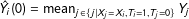
Second, is the correspondence assumption, which restricts the class of models to those which, when predicting points similar in the space of the covariates, are similar in the space of potential outcomes. Denote a Lipschitz constant  $K_{\ell }$ , and two $k$ -dimensional points, $x$ and  $x^{\prime }$ , each measured in the space of the theoretical support of $X$ (and not necessarily near its empirical support). Also define a proper nondegenerate distance, such that $d(x,x^{\prime })=0$ for exact matching (i.e., where $x=x^{\prime }$ ) and $d(x,x^{\prime })>0$ for deviations from exact matching (i.e., where $x\neq x^{\prime }$ ). Then the correspondence assumption is $|m_{\ell }(x)-m_{\ell }(x^{\prime })|\leqslant K_{\ell }\cdot d(x,x^{\prime })$ . Models satisfying this assumption (after conditioning on predictors) have at least a minimal level of continuity, such as having bounded derivatives (see King and Zeng Reference King and Zeng2006; Iacus, King, and Porro Reference Iacus, King and Porro2011; Kallus Reference Kallus2018).

We combine these assumptions in this class of competing models (Iacus, King, and Porro Reference Iacus, King and Porro2011):

$$\begin{eqnarray}\begin{array}{@{}rclr@{}}{\mathcal{M}}\ & =\ & \{m_{\ell }:|m_{j}(\tilde{x})-m_{k}(\tilde{x})|\leqslant h,\quad j\neq k,\quad & \text{(fit)}\\ \ & \ & \;\text{and}~|m_{\ell }(x)-m_{\ell }(x^{\prime })|\leqslant K_{\ell }\cdot d(x,x^{\prime })\quad & \text{(correspondence)}\end{array}\end{eqnarray}$$

and define model dependence, for any two models $m_{j},m_{k}\in {\mathcal{M}}_{h}$ in this class and some point $x$ in the theoretical space of  $X$ , as $|m_{j}(x)-m_{k}(x)|$ (King and Zeng Reference King and Zeng2007).

2.5 Model Dependence Biases Even Unbiased Estimators

We show here how estimators that are unbiased but inefficient when applied to one model are biased in the presence of model dependence and common researcher behavior.

3.1 How Successful Matching Reduces Model Dependence

In three steps, we prove that successful matching reduces model dependence. First, we define the immediate goal of matching as finding a subset of the data closer to exact matching. Deviations from exact matching are known as imbalance. One way to measure imbalance is the average distance from each unit $X_{i}$ to the closest unit in the opposite treatment regime, $X_{j(i)}$ , i.e., where $j(i)=\operatorname{argmin}_{j|T_{j}=1-T_{i}}\,d(X_{i},X_{j})$ . Thus, for the original data, imbalance could be measured as $I(X)=\operatorname{mean}_{i\in \{i\}}\,d(X_{i},X_{j(i)})$ . For a particular (matched) data subset, $\mathbb{X}$ , imbalance is $I(\mathbb{X})$ . Matching methods reduce imbalance when successful, so that $I(\mathbb{X})<I(X)$ .

Second, we prove that the level of imbalance in a data set bounds the degree of model dependence in estimating SATE. Denote an estimator of SATE, constructed using model $m_{j}\in {\mathcal{M}}$ , as $\hat{\unicode[STIX]{x1D70F}}(m_{j})$ , and similarly for the treatment effect $\widehat{\text{TE}}_{i}(m_{j})$ . Then:

(2) $$\begin{eqnarray}\displaystyle |\hat{\unicode[STIX]{x1D70F}}(m_{j})-\hat{\unicode[STIX]{x1D70F}}(m_{k})| & = & \displaystyle \mathop{\text{mean}}_{i\in \{i\}}|\widehat{\text{TE}}_{i}(m_{j})-\widehat{\text{TE}}_{i}(m_{k})|\nonumber\\ \displaystyle & {\leqslant} & \displaystyle \mathop{\text{mean}}_{i\in \{i\}}|m_{j}(X_{i})-m_{k}(X_{i})|\nonumber\\ \displaystyle & = & \displaystyle \mathop{\text{mean}}_{i\in \{i\}}|[m_{j}(X_{i})-m_{j}(X_{j(i)})]+[m_{k}(X_{i})-m_{k}(X_{j(i)})]+[m_{j}(X_{j(i)})-m_{k}(X_{j(i)})]|\nonumber\\ \displaystyle & {\leqslant} & \displaystyle \mathop{\text{mean}}_{i\in \{i\}}[|m_{j}(X_{i})-m_{j}(X_{j(i)})|+|m_{k}(X_{i})-m_{k}(X_{j(i)})|+|m_{j}(X_{j(i)})-m_{k}(X_{j(i)})|]\nonumber\\ \displaystyle & {\leqslant} & \displaystyle (K_{j}+K_{k})\mathop{\text{mean}}_{i\in \{i\}}\,d(X_{i},X_{j(i)})+h.\end{eqnarray}$$

Finally, Equation (2) implies, if matching is successful in reducing imbalance, that the bound on model dependence is lower in the matched subset than the original data:

(3) $$\begin{eqnarray}|\hat{\unicode[STIX]{x1D70F}}(m_{j})-\hat{\unicode[STIX]{x1D70F}}(m_{k})|\leqslant I(\mathbb{X})<I(X)\end{eqnarray}$$

which thus establishes how matching reduces the problem of model dependence.

3.2 Matching Methods

We briefly describe here PSM, and two other matching methods representative of the large variety used in the literature. We first present the simplest and most widely used version of each of the three methods and then discuss more rarely used refinements of PSM. We also report on a content analysis we conducted of the prevalence of these refinements across applied literatures.

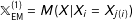
Technical Description

Each method we define here represents one of the two existing classes of matching methods: Mahalanobis Distance Matching (MDM) is one of the longest standing matching methods that can fall within the Equal Percent Bias Reducing (EPBR) class (Rubin Reference Rubin1976; Rubin and Stuart Reference Rubin and Stuart2006) and Coarsened Exact Matching (CEM) is the leading example within the Monotonic Imbalance Bounding (MIB) class (Iacus, King, and Porro Reference Iacus, King and Porro2011). PSM can also be EPBR, if used with appropriate data.

First define a function that prunes all observations from $X$ that do not meet specified conditions: $\mathbb{X}_{\ell }=M(X|A_{\ell },T_{i}=1,T_{j}=0,\unicode[STIX]{x1D6FF})\equiv M(X|A_{\ell })\subseteq X$ , where $\mathbb{X}_{\ell }$ is the subset of rows of $X$ produced by applying matching method  $\ell$ , given condition  $A_{\ell }$ . For example, under exact matching 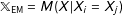$\mathbb{X}_{\text{EM}}=M(X|X_{i}=X_{j})$ ; under one-to-one exact matching with replacement $\mathbb{X}_{\text{EM}}^{(1)}=M(X|X_{i}=X_{j(i)})$ . The nonnegative parameter $\unicode[STIX]{x1D6FF}$ takes on a different meaning in each matching method, where  $\unicode[STIX]{x1D6FF}=0$ is the best matched subset of $X$ that can be produced according to method  $\ell$ . Since $\unicode[STIX]{x1D6FF}$ is an adjustable parameter, the three methods below can be thought of as producing a sequence of matched sets, indexed by  $\unicode[STIX]{x1D6FF}$ .

Under MDM,

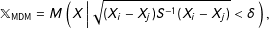$$\begin{eqnarray}\mathbb{X}_{\text{MDM}}=M\left(X\left|\,\sqrt{(X_{i}-X_{j})S^{-1}(X_{i}-X_{j})}<\unicode[STIX]{x1D6FF}\right.\right),\end{eqnarray}$$

given a “caliper” $\unicode[STIX]{x1D6FF}$ (Rosenbaum and Rubin Reference Rosenbaum and Rubin1985a; Stuart and Rubin Reference Stuart and Rubin2008), and sample covariance matrix $S$ of the original data matrix  $X$ . (MDM is commonly chosen for methods articles, where the standardization makes the variables unitless; in applications, metrics such as Euclidean better enable a researcher to represent knowledge of the underlying variables and their relative importance by scaling  $X$ .)

Under CEM, $\mathbb{X}_{\text{CEM}}=M[X\mid C_{\unicode[STIX]{x1D6FF}}(X_{i})=C_{\unicode[STIX]{x1D6FF}}(X_{j})]$ , where $C_{\unicode[STIX]{x1D6FF}}(X)$ has the same dimensions as $X$ but with coarsened values. The parameter $\unicode[STIX]{x1D6FF}$ represents a chosen coarsening such that $\unicode[STIX]{x1D6FF}=0$ is fine enough so that $C(X)=X$ , and larger values of $\unicode[STIX]{x1D6FF}$ represent coarser recordings for some or all variables (larger values of $\unicode[STIX]{x1D6FF}$ are not necessarily ordered). Continuous covariates could be coarsened at “natural breakpoints”, such as high school and college degrees in years of education, poverty level for income, etc. Discrete variables can be left as is or categories can be combined, such as when data analysts combine strong and weak Democrats into one category and strong and weak Republicans into another. (Variables can also be coarsened in groups of related variables, such as requiring the sum of three dichotomous variables to be equal.)

Finally, under PSM, $\mathbb{X}_{\text{PSM}}=M(X\mid |\hat{\unicode[STIX]{x1D70B}}_{i}-\hat{\unicode[STIX]{x1D70B}}_{j}|<\unicode[STIX]{x1D6FF})$ , where 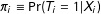$\unicode[STIX]{x1D70B}_{i}\equiv \Pr (T_{i}=1|X_{i})$ is the scalar “propensity score”, in practice almost always estimated by assuming a logistic regression model $\hat{\unicode[STIX]{x1D70B}}_{i}=(1+e^{-X_{i}\hat{\unicode[STIX]{x1D6FD}}})^{-1}$ . Most important here is the reduction of the $k$ dimensional $X_{i}$ to the scalar $\unicode[STIX]{x1D70B}_{i}$ before measuring the distance.

4.1 Different Experimental Ideals for Matching Methods

Consider two experimental designs. First, under a fully blocked randomized experimental design (FB), such as a matched pair randomized experiment, treated and control groups are blocked at the start exactly on the observed covariates. Imbalance in these experiments is thus always 0 by design, just as what exact matching tries to accomplish after the fact, but without having to prune any observations: $X_{\text{FB}}=M(X_{\text{FB}}|X_{i}=X_{j})$ , which implies $I(X_{\text{FB}})=0$ . Second, under a completely randomized experimental design (CR), treatment assignment $T$ depends only on the scalar probability of treatment $\unicode[STIX]{x1D70B}$ for all units, and so is random with respect to  $X$ . In any one sample, random does not mean zero imbalance (except by rare coincidence or in asymptotic samples): $I(X_{\text{CR}})\geqslant 0$ . For simplicity, we also use the term “completely randomized” to describe partially blocked designs, such as when a constant probability of treatment is assigned to units within each of several strata, so that assignment is random, and potentially imbalanced, with respect to $(X|\unicode[STIX]{x1D70B})\neq X$ .

The difference between the two experimental ideals is crucial since, compared to a completely randomized experimental design, a fully blocked randomized experimental design has more power, more efficiency, lower research costs, more robustness, less imbalance, and—most importantly from the perspective here—lower model dependence and thus less bias (Box, Hunter, and Hunter Reference Box, Hunter and Hunter1978; Greevy et al. Reference Greevy, Lu, Silver and Rosenbaum2004; Imai, King, and Stuart Reference Imai, King and Stuart2008; Imai, King, and Nall Reference Imai, King and Nall2009). For example, Imai, King, and Nall (Reference Imai, King and Nall2009) found that standard errors differed in their data between the two designs by as much as a factor of six. Indeed, “for gold standard answers, complete randomization may not be good enough, except for point estimation in very large experiments” (Rubin Reference Rubin2008a). Of course, the discrepancy between the estimate and the truth in the one data set a researcher gets to analyze is far more important to that researcher than what happens across hypothetical repeated samples from the same hypothetical population (cf. Gu and Rosenbaum Reference Gu and Rosenbaum1993).

Matching methods such as MDM and CEM approximate a fully blocked experimental design (Iacus, King, and Porro Reference Iacus, King and Porro2011, p. 349) because they come with adjustable parameters that can be set to produce the same result as exact matching, and thus zero imbalance. In particular, $\mathbb{X}_{\text{EM}}=M(X|A_{\text{CEM}},\unicode[STIX]{x1D6FF}=0)=M(X|A_{\text{MDM}},\unicode[STIX]{x1D6FF}=0)$ . However, this same calculation shows that PSM approximates merely a completely randomized experiment, and thus has potentially higher imbalance. That is, because $\mathbb{X}_{\text{EM}}\subseteq M(X|A_{\text{PSM}},\unicode[STIX]{x1D6FF}=0)$ , it follows that $I(\mathbb{X}_{\text{EM}})\leqslant I(\mathbb{X}_{\text{PSM}})$ , and strictly less than except for the unusual special cases (see also Rubin and Thomas Reference Rubin and Thomas2000). Moreover, the fact that CEM and MDM approximate a fully blocked experiment means that each has the ability to achieve lower levels of imbalance, model dependence, and bias than PSM.

4.2 The Inadequacy of PSM Theory

The original theoretical justification given for PSM was based on the proof that unconfoundedness conditional on the raw covariates, $Y(0)\bot T\mid X$ , along with overlap and SUTVA, implies unconfoundedness conditional on the scalar propensity score, $Y(0)\bot T\mid \unicode[STIX]{x1D70B}$ (Rosenbaum and Rubin Reference Rosenbaum and Rubin1983, Theorem 1). With this result, Rosenbaum and Rubin use the identification result in Equation (1) and show that a PSM matched sample can be used to produce an unbiased estimate of SATT or SATE, conditional on one model used for estimation. The motivation for this calculation is that it is supposedly easier to match on the scalar $\unicode[STIX]{x1D70B}$ than the $k$ -dimensional  $X$ . Although this is not the case for the exact matches required by the theorem if $X$ contains at least one continuous variable, it may be easier to find closer matches in one dimension than  $k$ .

Unfortunately, this proof, although mathematically correct, is either of little use or misleading when applied to real data. First, as Section 2.5 shows, conditioning on a single model is inappropriate, because users do no such thing. The point of observational data analysis is to discover the data generation process, and so researchers reasonably try many approaches and models. Yet, the theorem encourages researchers to settle for the lower standards of approximating only complete randomization and only average levels of imbalance (across experiments that will never be run), rather than a fully blocked experiment and balance in their own samples guaranteed to reduce model dependence. Balancing on $\unicode[STIX]{x1D70B}$ only is unbiased but inefficient ex ante, leaving researchers with more model dependence, discretion, and bias ex post.

The original idea behind PSM (and the proof) would have been somewhat more useful if it were reversed—if unconfoundedness (and matching) on $\unicode[STIX]{x1D70B}$ implied unconfoundedness on $X$ —but this cannot be proven because it is false. Although reducing model dependence requires reducing imbalance with respect to  $X$ , balancing only on $\unicode[STIX]{x1D70B}$ does not balance $X$ (since it is blind to variation in $X|\unicode[STIX]{x1D70B}$ ). More importantly, in sample, equality between any two estimated scalar propensity scores, $\hat{\unicode[STIX]{x1D70B}}_{i}=\hat{\unicode[STIX]{x1D70B}}_{j}$ , does not imply that the two corresponding $k$ -dimensional covariate vectors are matched exactly, $X_{i}=X_{j}$ —even though exact matching on the covariates $X_{i}=X_{j}$ does imply that the propensity scores are exactly matched $\hat{\unicode[STIX]{x1D70B}}_{i}=\hat{\unicode[STIX]{x1D70B}}_{j}$ .

4.3 Illustration

We now simulate 1,000 data sets, each of which mixes data from three separate sources: (1) a matched pair randomized experiment, (2) a completely randomized experiment, (3) observations that, when added to the first two components, make the entire collection an imbalanced observational data set. We then study whether MDM and PSM prune individual observations in the correct order—starting with those at the highest level of imbalance (data set 3) to the lowest (data set 1). For clarity, we use two covariates (using more covariates generates patterns like those we present here, only stronger).

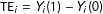
To fix ideas, we display one of our 1,000 data sets in the left panel of Figure 1, which highlights its three parts in separate colors. In blue in the upper right is the matched pair experiment with 25 treated units drawn uniformly from the $[-2,2]\times [-2,2]$ square and 25 control units which are slightly jittered versions of each of these treated units. In red, at the bottom right is a completely randomized experiment, with 50 random observations drawn uniformly from the $[-2,2]\times [-8,-4]$ rectangle and with 25 of these randomly assigned to treatment and 25 to control. Finally, we simulate part of an imbalanced observational study by adding 50 control observations in black, drawn uniformly from the $[-6,-4]\times [-8,2]$ square, and without corresponding randomly drawn (or otherwise overlapping) treated units.

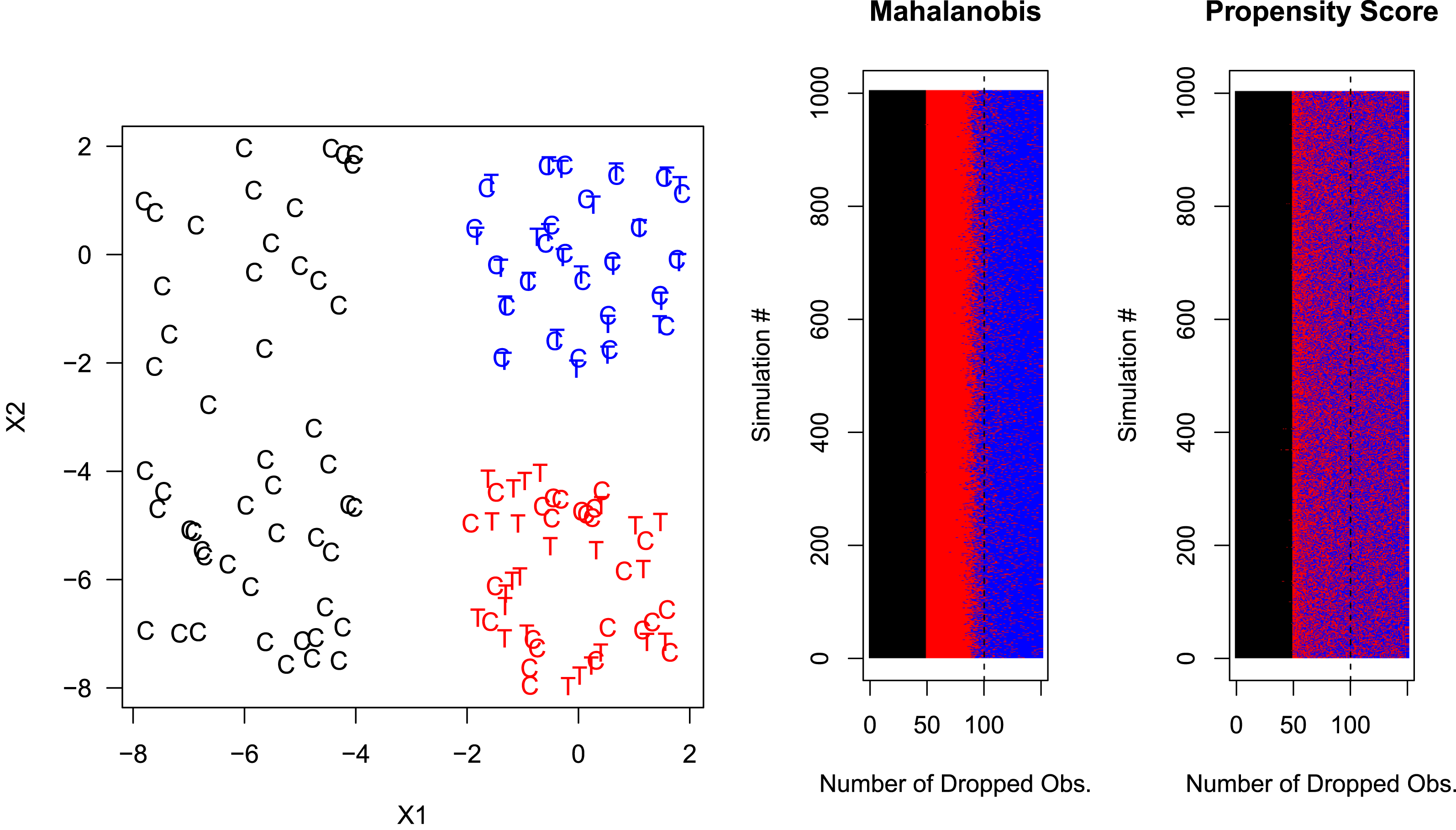
Figure 1. Finding experiments hidden in observational data, with PSM, but not MDM, blind to information from full blocking. Left panel: one (of 1,000) randomly generated data sets from a matched pair randomized experiment (in blue), a completely randomized experiment (in red), and control units from an imbalanced observational data set (in black). Right Panels: Each of the 1,000 simulations is represented by a separate row of pixels, color-coded by experiment type to indicate the order (from left to right) of which observations are pruned by MDM (left) and PSM (right).

We apply PSM and MDM, as per Section 3.2, to each data set, and iteratively remove the (next) worst observation as defined by each matching method. In the two panels at the right of Figure 1, each row of pixels stands for one simulated data set, with each individual pixel in a row representing one pruned observation color-coded by data set type. The results show that both MDM and PSM do well at removing the 50 control units that lack common support with any treated units (black is separate in both). MDM is able to separate the fully randomized experiment from the matched pair experiment (red is clearly separated from blue) but PSM is unable to separate the more informative matched pair experiment from the fully randomized experiment (red and blue are mixed).

In an application, a researcher may prefer to prune only the control units from the left part of the graph and no others. This would be best if SATT were the quantity of interest or, in some cases, to ensure that the variance is not increased too much by not pruning further. However, if the researcher chooses to prune more, and is willing to estimate FSATT, then using PSM would be a mistake. This simulation clearly shows that PSM cannot recover a matched pair experiment from these data. At best, it can recover something that looks like a fully randomized experiment, meaning that the covariates can no longer predict treatment on average. This is useful, since it makes possible estimation that is unbiased before conditioning on the treatment assignment. However, by definition some model dependence and researcher discretion remains which, when combined can lead to bias. The ideal is a fully blocked experiment, which is approximated by exact matching, not merely overlapping data clouds.

5.1 The Dangers of Random Matching

We show here that random pruning, a process of deleting observations in a data set independent of $(T,X)$ , not only reduces the information in the data; it also increases the level of imbalance. This may seem counterintuitive, and to our knowledge has not before been noted in the matching literature (cf. Imai, King, and Stuart Reference Imai, King and Stuart2008, p. 495). However, it is crucial, since pruning by PSM, when it succeeds in approximating complete randomization, is equivalent to random pruning. For intuition, we show this result in several ways (see also Section 1 in our Supplementary Appendix).

First, consider a completely randomized experiment with, for simplicity but no loss of generality, zero causal effects. That is, let $T$ be generated by Bernoulli random draws and $X$ by uniform random draws distributed over a nondegenerate space. If $k=3$ , then the expected distance of point $X_{i}$ to its nearest neighbor in the opposite treatment regime $X_{j(i)}$ (among $n_{1}$ such points) is $d(X_{i},X_{j(i)})=0.554n_{1}^{-1/3}$ (Bansal and Ardell Reference Bansal and Ardell1972). In a more general context, Abadie and Imbens (Reference Abadie and Imbens2006) show, in samples with $K$ continuous covariates from a distribution with bounded support, that the nearest neighbor in $X$ of a point is of order $n_{1}^{-1/K}$ . Thus, in either framework, when a matching method prunes observations randomly, $n_{1}$ declines, the distance increases, and imbalance $I(\mathbb{X})$ grows.

Second, for intuition, consider a simple discrete data set that happened to be perfectly balanced, with a treatment group composed of one male and one female, $M_{1},F_{1}$ , and a control group with the same composition, $M_{0},F_{0}$ . Then, randomly dropping two of the four observations leaves us with one matched pair among $\{M_{1},M_{0}\}$ , $\{F_{1},F_{0}\}$ , $\{M_{1},F_{0}\}$ , or $\{F_{1},M_{0}\}$ , with equal probability. This means that with 1/2 probability the resulting data set will be balanced ( $\{M_{1},M_{0}\}$ or $\{F_{1},F_{0}\}$ ) and with $1/2$ probability it will be completely imbalanced ( $\{M_{1},F_{0}\}$ or $\{F_{1},M_{0}\}$ ). Thus, on average in these data random matching will increase imbalance.

Finally, for a simple continuous example, consider a randomly assigned $T$ and a fixed univariate  $X$ . Consider, as a measure of imbalance, the squared difference in means between the treated and control group of  $X$ . The expected value of this measure (which equals the squared standard error of the difference in means) is proportional to $1/n$ . Thus, as we prune from this sample randomly, $n$ declines and our measure of imbalance increases.

Of course, if all the matching discrepancies are of the same size, pruning at random or by any other means will not change the average matching discrepancy (or most other measures of imbalance). But in more realistic simulations, and real data we have examined, random pruning increases imbalance. We also introduce a higher dimensional example with real data in Section 5.3.

5.2 Simulation

We now turn to a demonstration of how PSM generates model dependence and bias. We begin by hiding a completely randomized experiment within an imbalanced data set. Unlike Figure 1, we do not include a fully blocked experiment within these data. For each of two covariates, we randomly and independently draw 100 control units from a Uniform( $0,5$ ) and 100 treated units from Uniform( $1,6$ ). This leaves the overlapping $[1,5]\times [1,5]$ square as a completely randomized experiment and observations falling outside adding imbalance. We generate the outcome as $Y_{i}=2T_{i}+X_{i1}+X_{i2}+\unicode[STIX]{x1D716}_{i}$ , where $\unicode[STIX]{x1D716}\sim N(0,1)$ . We repeat the entire simulation 100 times. We assume, as usual, that the analyst knows the covariates necessary to achieve unconfoundedness but does not know the functional form.

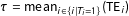
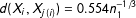
Figure 2. PSM Increases Model Dependence and Potential Bias. Top-left panel: the vertical axis measures model dependence as the average, over 100 data sets, of the variance in the causal effect estimate across 512 models applied to the same data. Top-right panel: the vertical axis shows the maximum estimated causal effect from 512 models applied to each of 100 data sets. For one simulated data set, the order of matches is indicated for MDM (bottom-left panel) and PSM (bottom-right panel).

To evaluate the methods, we compute both model dependence and potential for bias, each averaged over 100 simulated data sets. We measure model dependence by the variance in the estimate of the causal effect over 512 separate models (linear regression using every possible combination of $X_{1}$ and $X_{2}$ and their 3 second order and 4 third order effects) from the same simulated data set for each given caliper level; we do this for PSM and then also MDM as a comparison. The results, which appear in the top-left panel of Figure 2, show that at first the degree of model dependence drops for both MDM and PSM, but then, after PSM has pruned enough so that the PSM paradox kicks in, model dependence dramatically increases. Instead of benefiting from units being dropped, PSM is causing damage. (This is like walking into a shoe store, giving the cashier some money and, instead of handing you a new pair of shoes, he takes the shoes you walked in with.) Model dependence for MDM, as expected, declines monotonically as stricter calipers are applied and more units are pruned.

To show how the combination of model dependence and analyst discretion can result in bias, we implemented an estimator meant to simulate the common situation where the analyst chooses a preferred estimate to publish from many possible estimates. Suppose the researcher’s preferred hypothesis is that the causal effect is large, and that this preference intentionally or unintentionally affects their choice. Thus, for each caliper level of PSM and then MDM, we select the largest estimated treatment effect from among the estimates provided by the 512 possible specifications. The results, in the top-right panel of Figure 2, show that calipering initially does what we would expect by reducing the potential for bias for both MDM and PSM, with PSM even slightly outperforming MDM. However, as calipering continues, the PSM paradox kicks in, and PSM increases model dependence (as indicated in the top-left graph), the potential for bias with PSM dramatically grows even while the bias under MDM monotonically declines as we would expect and desire. (Although we do not show the graph, these patterns are unchanged for mean squared error as well.)

To provide intuition for how the paradox occurs in these data, we show which observations are matched and in which order in one of the 100 simulated data sets. Thus also in Figure 2, we plot $X_{1},X_{2}$ points from one simulated data set, with matches from MDM (bottom-left panel) and PSM (bottom-right panel) denoted by lines drawn between the points, colored in by when they were matched or pruned in the calipering process. (The outcome variable is ignored during the matching process, as usual.) Darker colors were pruned later (i.e., matched earlier).

As expected, the MDM results (bottom-left panel) show that treated (circles) and control (dots) pairs that are close to each other are matched first (or pruned last). These darker blue lines mostly appear within the (completely randomized) square in the middle. In stark contrast, PSM, in the bottom-right panel, finds many matches seemingly unrelated to local closeness of treated and control units and many even outside the middle square. The diagonal pattern in PSM dark lines comes from the propensity score logit which cannot distinguish high values of $X_{1}$ and low values of $X_{2}$ from low values of $X_{1}$ and high values of  $X_{2}$ .

Overall, the figure shows that PSM is trying to match globally—meaning it essentially has only one chance to get it right, rather than matching locally like other methods and having some additional degree of robustness. In fact, because the propensity score is outside the space of the original data, using it for analysis violates the congruence principle. This principle holds that the data space and analysis space should be the same. Statistical methods which violate this principle are known to generate nonrobust and counterintuitive properties (Mielke and Berry Reference Mielke and Berry2007).

5.3 Damage Caused in Real Data

In this section, we reveal the PSM paradox in real applications, with data selected and analyzed by others, including two published studies and a large number of others in progress. We obtained the data from the studies in progress by advertising to assist scholars in making causal inferences, in return for access to their data and a promise not to redistribute their data or publish their substantive results (or identities). For almost all the more than 20 data sets in progress we analyzed, we found patterns similar or analogous to the two we are about to present in detail. From this, we conclude that the PSM Paradox is prevalent in many real applications.

In this first published study we reanalyze, Finkel, Horowitz, and Rojo-Mendoza (Reference Finkel, Horowitz and Rojo-Mendoza2012) showed that civic education programs in Kenya cause citizens to have more civic competence and engagement and be more supportive of the political system, with $n=\text{3,141}$ survey responses, 1,347 of which received the program. They also measured a large number of socioeconomic, demographic, and leadership covariates. Second, Nielsen et al. (Reference Nielsen, Findley, Davis, Candland and Nielson2011) show that a sudden decrease in international foreign aid to a developing country (an “aid shock”) increases the probability of the onset of lethal conflict within that country. They collect data on developing countries from 1975 to 2006, in total representing $n=\text{2,627}$ country-years, including 393 (treated) aid shocks. The authors measure 18 pretreatment covariates representing national levels of democracy, wealth, population, ethnic and religious fractionalization, and prior upheaval and violence. Finally, we analyzed a large number of data sets obtained from scholars doing work in progress, which we received by trading offers of help with their analyses and promising not to cite or scoop them. The results of all sources of data yielded very similar conclusions to that from the two data sets we now reanalyze.

For both of the published studies we replicate, Figure 3 plots imbalance (vertically) by the number of pruned observations (horizontally). We measure imbalance (i.e., the difference between the empirical distribution of $X$ in the treated and control groups) by the “Mahalanobis Discrepancy,” proposed by Abadie and Imbens (Reference Abadie and Imbens2006), which as per Section 3.1 measures imbalance in the space of  $X$ .Footnote ⁵ In each plot, the open circle at the left summarizes the imbalance in original data set. For reference, we also add a solid triangle that summarizes the level of imbalance that would be present if $T$ were assigned via complete randomization.

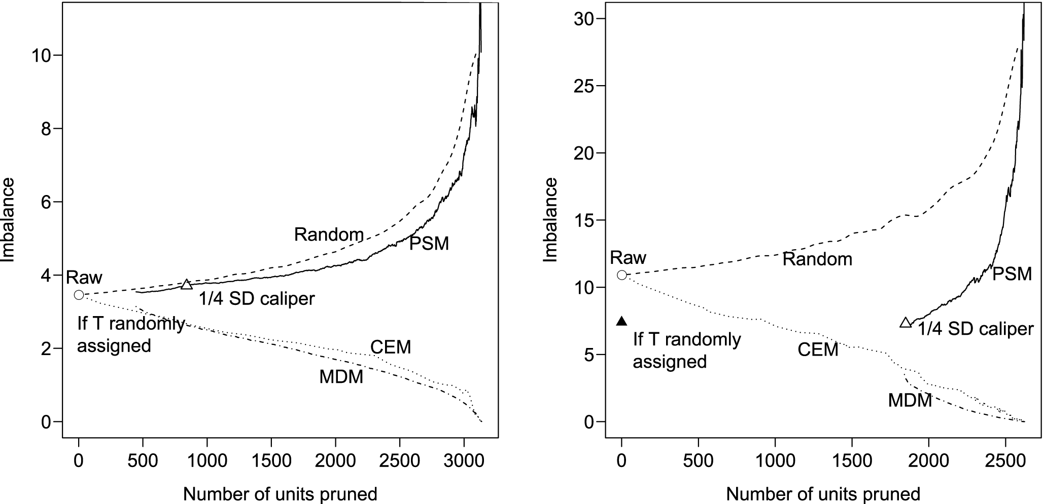
Figure 3. Imbalance-matched sample size graph, with data from Finkel, Horowitz, and Rojo-Mendoza (Reference Finkel, Horowitz and Rojo-Mendoza2012) for the left panel and Nielsen et al. (Reference Nielsen, Findley, Davis, Candland and Nielson2011) for the right.

The one-to-one PSM analysis (which in the case of Nielsen et al. Reference Nielsen, Findley, Davis, Candland and Nielson2011 is the published result and in both cases is estimated by all main effects in a logit model) is represented by the left end of the solid line. In the left panel, PSM’s initial result is worse than the original data; in the right panel it is an improvement, as Nielsen et al. (Reference Nielsen, Findley, Davis, Candland and Nielson2011) report. However, consider what happens in either data set if we caliper off the worst match according to the propensity score metric (i.e., the largest value of $|\hat{\unicode[STIX]{x1D70B}}_{i}-\hat{\unicode[STIX]{x1D70B}}_{j}|$ across all matched pairs), recalculate the level of imbalance, and repeat. These results, which are represented by the full black line in each panel, reveal the PSM paradox kicking in immediately and continuing until no data is left: That is, the more strict we are in applying PSM, the worse imbalance gets. (In a few of the unpublished data sets we analyzed that had much worse initial imbalance, PSM helped for initial pruning and then started increasing imbalance as in these graphs; simulated examples of this pattern appear in Section 3 of our Supplementary Appendix.)

If we use the venerated practice of setting the caliper to $1/4$ of a standard deviation of the propensity score (Rosenbaum and Rubin Reference Rosenbaum and Rubin1985a), imbalance is worse than the basic PSM solution for the left panel and provides no improvement for the right panel. Following the strictures of PSM even more closely, in the hopes of finding better balance and less model dependence, accomplishes precisely the opposite.

For comparison, in each graph, we also prune via MDM (dot-dashed line) and CEM (dotted line). For MDM, we do one-to-one matching (and so the line starts at the same horizontal point as PSM) and then caliper off the observations with the largest Mahalanobis distance, recompute imbalance, and repeat. For CEM, we begin with the loosest possible coarsening, so that all data fall in a single stratum and no observations are pruned (and so the line starts from the original data). We then randomly select a variable, add one cut-point to its coarsening (always arranging the cutpoints so they divide the space between the minimum and maximum values into equal sized bins), and compute the imbalance metric. Additional cutpoints eventually lead to more observations being dropped.

As can be seen in both panels in Figure 3, the MDM and CEM lines both tend downward through their entire range with no hint of the paradox that would be represented by an upward turn like PSM: in this case, the trade-off is as it should be, in that one can reasonably choose any point along this frontier to do an analysis. (The figure also includes a dashed line marked “Random” representing the average of a sequence of data sets constructed by random pruning; as with the simpler examples in Section 5.1, the figure shows that random pruning increases imbalance.)

6.1 Advice for PSM Users

Our results indicate that those who wish to continue to use PSM, perhaps due to familiarity or convenience in their established work flows, would improve their work by adhering to the following points.

First, researchers using any matching method must explicitly scale variables to represent their importance (in terms of prior knowledge about effects on the outcome variable), since imbalance combines with importance to affect bias. Some claim that PSM automatically solves the problem of scaling when some variables have unknown importance, but this is untrue. Scaling is less transparent with PSM than with MDM, Euclidean distance matching, or especially CEM, but PSM users cannot avoid representing prior research in the scaling of their variables. Ignoring the issue is an arbitrary choice that may well increase bias.

Second, choosing PSM introduces avoidable risks and so researchers should report on what techniques they used to avoid the resulting problems. They should clarify how much imbalance, and therefore model dependence and bias, is left after applying PSM, especially compared to how much existed in the original data. Readers deserve to know that the researcher is not making imbalance worse due to the PSM paradox. In particular, setting a more restrictive caliper, supposedly to meet the conditions of PSM more precisely, may well increase imbalance. We recommend the routine reporting of diagnostic plots like those in Figure 3. Even carefully using PSM will likely be suboptimal compared to other matching methods, but it can sometimes be an improvement relative to the original data if used much more carefully than has been common practice (see Section 3.2).

Third, researchers should be aware that PSM can help the most in data where valid causal inferences are least likely (i.e., with high levels of imbalance) and may do the most damage in data that are well suited to making causal inferences (i.e., with low levels of imbalance). PSM is better justified (i.e., still suboptimal but not as much) when very large sample sizes are available after matching, both so as not to go past the point of complete randomization and so that the difference after matching between fully blocked and completely randomized experiments is smaller and less consequential.

Finally, researchers should understand what happens when combining PSM with other matching methods, as is sometimes recommended in the literature. One option is running PSM first, being careful to stop pruning before the PSM paradox kicks in, followed by matching directly on $X$ with another method. The matched sample will likely be close to only applying the second method.

A second option is to precede PSM with exact or coarsened matching on a few important covariates. The advantage of this procedure is that its first step can take one closer to full blocking than PSM alone is capable of. Its disadvantage is that it makes applying PSM more dangerous: the closer the exact matching step comes to balancing all of  $X$ , the quicker pruning with PSM will lead to the paradox and begin to increase imbalance.

A final option that has been suggested is iteratively checking balance and respecifying the propensity score regression (see Section 3.2). To the extent that these methods wind up matching more on $X$ than the propensity score, they may sometimes perform better than PSM alone, although not as well as methods freed from the constraint of unnecessarily passing through a one dimensional propensity score. In addition to being used only rarely in the applied literature (see Section 3.2), the theoretical properties of most of these approaches have not been studied. We provide some information about this approach by replicating the PSM analyses in this paper and in our Supplementary Appendix with the automated iterative procedure proposed in Imbens and Rubin (Reference Imbens and Rubin2015, chap. 13) and several others. We find little change, and more damage the more the method relies on PSM. For one example, we replicated the top three graphs from Figure 5 in our Supplementary Appendix with the Imbens–Rubin iterative procedure and found almost imperceptible differences.

6.2 Advice for Users of Other Matching Methods

Any matching method that prunes in a manner independent of the covariates (and thus is pruning randomly) can increase imbalance. With PSM, this point, which we call the PSM paradox, kicks in after the point of complete randomization is reached, since PSM is blind to information in $X$ not represented in the propensity score.

For other matching methods that can detect all differences in  $X$ , pruning after approximating complete randomization will continue to help reduce imbalance. Much later, after we prune enough to approximate a fully blocked experimental design, all information in $X$ will have been exhausted. At that point, all the units are exchangeable aside from their treatment assignment and so any further pruning can only take place at random (with respect to  $X$ ), which would increase imbalance. Of course, at full blocking—such as for example after exact matching—it is obvious that further pruning serves no useful purpose. We can however contrive instances where the paradox occurs with other methods, and conceivably researchers might be fooled. To illustrate, we offer two simulations in Section 4 of our Supplementary Appendix that involve pruning with MDM after using all information in  $X$ .

In the end, discarding data, which violates a basic conceptual principle of statistical inference, must be done only if you get something positive from it, such as reducing imbalance. In all applications and with all matching methods, researchers should closely study the data, the units pruned, how much imbalance and model dependence is left, and whether the process of pruning is improving or degrading inferences.

In choosing a matching method, the most important considerations are (a) ensuring one can match on all of  $X$ , so that it is at least possible to approximate a fully blocked randomized experiment, and (b) being able to encode prior knowledge about the relative importance of the variables and their combinations. For data sets with solely continuous variables, Euclidean distance matching should work well. For data with continuous, discrete, and mixed variables (such as continuous variables with natural breakpoints), CEM is the most natural; it is also considerably faster than other methods and so also works well for much larger data sets. Many other approaches aside from PSM also fit these criteria.