


1 Introduction
Ideological scaling methods have long been a mainstay in legislative studies, and scholars are increasingly applying these methods to disparate sources of data beyond roll-call votes. The goal is to extract a simple, low-dimensional summary measure of ideology from votes, survey responses, or other types of political data.Footnote 1 Typically, researchers seek to align political actors on a simple left–right political spectrum, which can be used to characterize public opinion and to study representation. Despite the prevalence of ideological scaling methods, there remain unresolved debates about how to interpret the resulting estimates—especially when applied to noninstitutional actors such as survey respondents.
First, there is debate over the dimensionality of political conflict. In the study of American politics, the default setting is to estimate a one-dimensional left–right model, in line with conventional wisdom about the dimensionality of contemporary Congress (cf. Poole and Rosenthal Reference Poole and Rosenthal1997). Yet, some researchers suggest as many as eight dimensions are needed to explain Congressional voting patterns (Heckman and Snyder Reference Heckman and Snyder1997), and recent empirical work on American institutions has found value in accounting for multidimensional preference structures (Jeong et al. Reference Jeong, Lowry, Miller and Sened2014; Crespin and Rohde Reference Crespin and Rohde2010). Other scholars argue that one dimension is not enough, because voters think about politicians in multiple dimensions rather than just one (Ahler and Broockman Reference Ahler and Broockman2018). This is perhaps because the political preferences of voters are best captured by two or more dimensions (Treier and Hillygus Reference Treier and Hillygus2009).
Second, there is debate over how constrained attitudes are in the public relative to politicians, which determines the interpretability of any ideal point estimates. Some authors claim that most citizens do not have well-formed political opinions, let alone opinions that can be meaningfully placed on a left–right spectrum (e.g., Converse Reference Converse and Apter1964; Kinder Reference Kinder, MacKuen and Rabinowitz2003). In an extreme view, policy attitudes are unstable and entirely idiosyncratic, meaning that scaling methods have little hope of recovering a useful estimate of ideology. A slightly weaker formulation is that citizen preferences are somewhat constrained, but that they are not amenable to a low-dimensional summary (Broockman Reference Broockman2016; Lauderdale, Hanretty, and Vivyan Reference Lauderdale, Hanretty and Vivyan2018). In this case, only a small portion of variance in survey responses can be explained by a single dimension.
A common sentiment is that public opinion is multidimensional, while political conflict among the parties is one-dimensional. A natural implication is that a higher-dimensional model should better describe public opinion data. Under this view, low constraint and multidimensionality are synonyms (Broockman Reference Broockman2016). A population exhibiting high constraint must also have one-dimensional political preferences, and a population exhibiting low constraint has multidimensional preferences.
In this paper, we seek to distinguish between these two notions, dimensionality and constraint, in the context of ideal point models. We point out that dimensionality refers to the effective number of separate issues that are commonly understood and acted upon by all voters. In the language of Heckman and Snyder (Reference Heckman and Snyder1997), the dimensionality is the number of “attributes” of policy choices that are needed to rationalize votes. Constraint, in contrast, refers to how much political actors rely on these attributes (e.g., left–right ideology) in forming opinions on particular policies rather than idiosyncratic reasons. An example of an idiosyncrasy in American politics would be an otherwise fiscally conservative voter favoring generous unemployment benefits (perhaps because they were once unemployed themselves). In a highly constrained population of actors, knowing an actor’s opinions on one set of issues should enable accurate prediction of further opinions, relative to an appropriately chosen null model. In an unconstrained population, most policy attitudes are idiosyncratic and thus unrelated to each other.
From this new perspective, constraint and dimensionality are orthogonal concepts. Theoretically, any population can exhibit any level of constraint with any level of dimensionality. Instead of unidimensionality and high constraint going hand in hand, we could in fact observe low constraint and unidimensionality together or high constraint with multidimensionality. Thus, even if we are convinced a population like the mass public exhibit low constraint on average, it remains an empirical question whether public opinion should be characterized by one or more dimensions. Similarly, a high level of constraint in Congress does not guarantee that members of Congress vote in a manner consistent with one-dimensional political preferences.
Drawing on these ideas, we propose an out-of-sample model validation procedure for ideal point models that enables us to estimate the dimensionality of political preferences and the associated level of constraint for a given population. In contrast, extant model validation efforts in the literature have focused on in-sample fit or ad hoc measures of out-of-sample fit. We document evidence of significant overfitting in ideal point models, illustrating the importance of a theoretically motivated out-of-sample validation strategy.
We apply the validation procedure to the workhorse quadratic-utility ideal point model commonly used to estimate ideal points. With an array of datasets that encompass both politicians and the public, we draw three main empirical conclusions.
First, we find no evidence that multidimensional models of ideal points explain preferences better than one-dimensional models—in fact, due to overfitting, higher-dimensional models can perform worse than a model that does not estimate ideal points at all. Second, we find that ideal point models are considerably less predictive when applied to the public. In contrast with politicians, voter responses are dominated by idiosyncratic, rather than ideological, preferences. This suggests the public has low constraint, at least relative to politicians. We also document some heterogeneity in the public, suggesting that ideal point models are more informative about individual issue attitudes for some groups than for others. Third, we decompose this difference in model performance between the public and politicians. We find that nearly all of the divergence can be attributed to differences in the constraint of the actors, rather than different measurement tools or disparate incentives faced by the actors. When applied to high-quality survey data of politicians, scaling methods perform nearly as well as when applied to roll-call votes. We also take advantage of paired data sources of politicians and the public to show that this conclusion is not driven by differences in the agenda or survey design.
These results suggest caution in applying ideal point estimation methods to surveys in the mass public. The resulting estimates do indeed explain some of the variation in stated preferences. However, the variance in preferences for particular policies that is explained by ideal points is considerably lower than for politicians. Idiosyncratic preferences—rather than spatial preferences—tend to dominate voter attitudes. These results suggest that scholars should not limit themselves to ideal point estimates when studying political attitudes in the mass public (Ahler and Broockman Reference Ahler and Broockman2018).
The rest of the paper is structured as follows. First, we discuss the differences between dimensionality and constraint. Then, we propose out-of-sample validation procedures to measure them. Next, we address the debate about the dimensionality of political conflict. Finally, we examine differences in constraint across populations and contexts, while addressing possible explanations for the divergence between elites and the mass public.
2 Constraint and Multidimensionality
At least as far back as Converse (Reference Converse and Apter1964), scholars of public opinion have been aware of the fact that American voters do not fit as cleanly inside ideological lines as, say, members of Congress or state legislators. A common sentiment in this literature is that voters’ policy attitudes are not derived from a coherent ideological framework. Instead, attitudes are idiosyncratic or at least not structured in the same way as politicians’. This perspective emphasizes a notion of ideology as constraint. Constraint here refers to the degree to which policy attitudes on some issues are predictive of policy attitudes on other issues. For example, if there is high degree of ideological constraint in the population, then knowing a voter’s preferences for welfare spending should allow one to infer their preferred tax rate. If there is a low degree of constraint, then knowing the voter’s preference about the welfare spending tells us little about their preferred tax rate.
The primary evidence for the lack of constraint comes from the low interitem correlations between survey responses (Converse Reference Converse and Apter1964) and lack of knowledge about which issues “go together” (Freeder, Lenz, and Turney Reference Freeder, Lenz and Turney2019). Summarizing one view, Kinder (Reference Kinder, MacKuen and Rabinowitz2003, 16) writes that “Converse’s original claim of ideological naïveté stands up quite well, both to detailed reanalysis and to political change.” This view implies that a one-dimensional spatial model is simply not useful for understanding public opinion.
In contrast, some scholars have attempted to salvage the idea of constrained voters by arguing that a multidimensional model provides a more reasonable picture of how voters perceive politics. For example, Treier and Hillygus (Reference Treier and Hillygus2009) write, “Our analysis documents the multidimensional nature of policy preferences in the American electorate… [F]ailing to account for the multidimensional nature of ideological preferences can produce inaccurate predictions of voting behavior.” In some of these arguments, the additional dimensions are considered to be just as important as the first. For instance, Lauderdale et al. (Reference Lauderdale, Hanretty and Vivyan2018) claim that including a second dimension nearly doubles how much variance in stated preferences is attributable to ideology.Footnote 2 An implied sentiment is that observed levels of constraint increase with a more flexible notion of ideology that encompasses multiple dimensions.
The goal of this paper is to distinguish between these two notions, constraint and multidimensionality, and to provide rigorous measures of them. The dimensionality of policy attitudes refers to the number of distinct underlying issues that are common to all people responding to the survey (or voting on roll-call votes). For example, we may think of policies as occupying a space with both “economic” and “moral” issue dimensions that are understood in the same way by all political actors. Multidimensionality simply refers to the presence of multiple such issues. The level of constraint, in contrast, refers to how much knowledge of someone’s policy attitudes on some issues helps us predict their policy attitudes on other issues through the common policy space. There may be many idiosyncratic factors affecting individuals’ policy attitudes that have nothing to do with the common policy space. The level of constraint refers to how much variance the common policy space explains relative to the idiosyncratic components.
There are no trade-offs between constraint and multidimensionality: either can appear with or without the other. Whether voters have multidimensional preferences has little to do (logically) with whether they have constrained preferences. A natural implication of this point is that there is a limit to how well we can predict political attitudes from other attitudes, since modeling additional dimensions of ideology has diminishing returns.
2.1 Formalizing Constraint and Multidimensionality
We now formalize constraint and multidimensionality in the context of canonical ideal point models. This will result in some observable implications that we can use to empirically identify the level of constraint and dimensionality in a population given a sample of its political choices.
We couch our discussion in terms of the familiar quadratic-utility spatial voting model used in Clinton, Jackman, and Rivers (2004, hereafter CJR).Footnote
3
Specifically, we will suppose the political actors we are studying—whether they be members of Congress, survey respondents, and so on—have an ideal point
 $\gamma _{i}$
located in some common D-dimensional Euclidean space. When considering a choice between two policy proposals, a “yea” policy located at point
$\gamma _{i}$
located in some common D-dimensional Euclidean space. When considering a choice between two policy proposals, a “yea” policy located at point
 $\zeta _{j}$
and a “nay” policy located at
$\zeta _{j}$
and a “nay” policy located at
 $\psi _{j}$
, voters’ utility is a function of the distance between their ideal point
$\psi _{j}$
, voters’ utility is a function of the distance between their ideal point
 $\gamma _{i}$
and the policy positions, plus a mean-zero idiosyncratic preference shock independently distributed across actors and proposals. Under the assumption of normally distributed shocks, it is simple to obtain an expression for the probability actor i chooses the yea option on choice j, denoted
$\gamma _{i}$
and the policy positions, plus a mean-zero idiosyncratic preference shock independently distributed across actors and proposals. Under the assumption of normally distributed shocks, it is simple to obtain an expression for the probability actor i chooses the yea option on choice j, denoted
 $y_{ij}=1$
. Averaging over preference shocks, it is given by
$y_{ij}=1$
. Averaging over preference shocks, it is given by
 $$ \begin{align} P(y_{ij} = 1 \mid \alpha_{j}, \beta_{j}, \gamma_{i}) &= \Phi(\alpha_{j} + \beta_{j} {{}}^{\mkern-1.5mu\mathsf{T}} \gamma_{i}), \end{align} $$
where
 $\alpha _{j}$
and
$\alpha _{j}$
and
 $\beta _{j}$
are functions of the policy locations and the distribution of shocks.Footnote
4
$\beta _{j}$
are functions of the policy locations and the distribution of shocks.Footnote
4
We use this model to characterize the distinction between multidimensionality and constraint. Implicit in the model is the dimensionality of the common policy space. The parameters
 $\gamma _{i}$
and
$\gamma _{i}$
and
 $\beta _{j}$
lie in some D-dimensional Euclidean space
$\beta _{j}$
lie in some D-dimensional Euclidean space
 $\mathbb {R}^{D}$
representing the space of possible policies. For instance, Treier and Hillygus (Reference Treier and Hillygus2009) consider a two-dimensional policy space to reflect economic and social issues. We might label the positive end of this space in both directions to refer to “conservative” policies, so an actor with
$\mathbb {R}^{D}$
representing the space of possible policies. For instance, Treier and Hillygus (Reference Treier and Hillygus2009) consider a two-dimensional policy space to reflect economic and social issues. We might label the positive end of this space in both directions to refer to “conservative” policies, so an actor with
 $\gamma _{i} = (-1.5, 3.2)$
would prefer “liberal” economic policies and “conservative” social policies.
$\gamma _{i} = (-1.5, 3.2)$
would prefer “liberal” economic policies and “conservative” social policies.
To further unpack this, focus on the linear predictor of actor i and choice j:
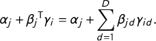 $$ \begin{align} \alpha_{j} + \beta_{j} {{}}^{\mkern-1.5mu\mathsf{T}} \gamma_{i} &= \alpha_{j} + \sum_{d=1}^{D} \beta_{jd}\gamma_{id}. \end{align} $$
Equation (2) suggests that choice j is analogous to a (generalized) linear regression. The “intercept”
 $\alpha _{j}$
and “coefficients”
$\alpha _{j}$
and “coefficients”
 $\beta _{j}$
change from choice to choice depending on the alternatives on offer, but the “covariates”
$\beta _{j}$
change from choice to choice depending on the alternatives on offer, but the “covariates”
 $\gamma _{i}$
stay the same for actor i across choices. For instance, the mapping from economic and moral preferences to a tax policy question will differ from how those same preferences map onto an immigration policy question (different intercepts and slopes), but the underlying economic and moral preferences (covariates) stay the same.
$\gamma _{i}$
stay the same for actor i across choices. For instance, the mapping from economic and moral preferences to a tax policy question will differ from how those same preferences map onto an immigration policy question (different intercepts and slopes), but the underlying economic and moral preferences (covariates) stay the same.
Thus, we can think of the dimensionality D as the number of underlying preferences needed to explain expected utilities. When D is small, there are only a few key attributes that meaningfully distinguish between policies in expectation—all of the other variables that determine utilities are too idiosyncratic to be organized into a common policy space. However, when D is large, there is a greater variety of systematic political conflict. The residual incentives for voting yea or nay are still idiosyncratic, but the systematic components of utility involve trade-offs between a higher number of issue dimensions. With high dimensionality, actors might be balancing preferences along, say, tax policy, morality policy, immigration policy, foreign policy, etc., provided these preferences are sufficiently uncorrelated.Footnote 5
If multidimensionality is the correct number of covariates needed to model expected choice in Equation (2), then constraint is the amount of variation those covariates can explain. As we alluded to previously, constraint captures the idea that knowing an actor’s ideal policy,
 $\gamma _{i}$
, improves our ability to predict their choices. In the linear regression analogy, constraint is similar to the
$\gamma _{i}$
, improves our ability to predict their choices. In the linear regression analogy, constraint is similar to the
 $R^{2}$
statistic: how much better we do in prediction after conditioning on the covariates
$R^{2}$
statistic: how much better we do in prediction after conditioning on the covariates
 $\gamma _{i}$
.
$\gamma _{i}$
.
To see precisely how knowledge of
 $\gamma _{i}$
might improve our ability to predict choices, recall that the probability of a yea vote conditional on
$\gamma _{i}$
might improve our ability to predict choices, recall that the probability of a yea vote conditional on
 $\gamma _{i}$
is given by Equation (1),
$\gamma _{i}$
is given by Equation (1),
 $P(y_{ij} = 1 \mid \alpha _{j}, \beta _{j}, \gamma _{i}) = \Phi (\alpha _{j} + \beta _{j} {{}}^{\mkern -1.5mu\mathsf {T}} \gamma _{i})$
. How does the probability of a yea vote change if we do not have knowledge of the ideal point
$P(y_{ij} = 1 \mid \alpha _{j}, \beta _{j}, \gamma _{i}) = \Phi (\alpha _{j} + \beta _{j} {{}}^{\mkern -1.5mu\mathsf {T}} \gamma _{i})$
. How does the probability of a yea vote change if we do not have knowledge of the ideal point
 $\gamma _{i}$
? To compute this, we must imagine drawing an actor at random, which means we must draw a value of their ideal point from the population distribution. For illustration, suppose we draw the ideal points from a standard multivariate normal:
$\gamma _{i}$
? To compute this, we must imagine drawing an actor at random, which means we must draw a value of their ideal point from the population distribution. For illustration, suppose we draw the ideal points from a standard multivariate normal:
 $\gamma _{i} \sim N(0, I_{D})$
. Then, the population average probability of a yea vote on choice j is given by
$\gamma _{i} \sim N(0, I_{D})$
. Then, the population average probability of a yea vote on choice j is given by
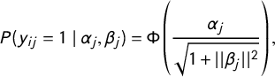 $$ \begin{align} P(y_{ij} = 1 \mid \alpha_{j}, \beta_{j}) &= \Phi\left(\frac{\alpha_{j}}{\sqrt{1 + ||\beta_{j}||^{2}}} \right), \end{align} $$
for all actors i. This is essentially an intercept-only probit model
 $\Phi (\delta _{j})$
with intercept
$\Phi (\delta _{j})$
with intercept
 $\delta _{j} = \alpha _{j} / \sqrt {1 + ||\beta _{j}||^{2}}$
that varies for each item j.Footnote
6
$\delta _{j} = \alpha _{j} / \sqrt {1 + ||\beta _{j}||^{2}}$
that varies for each item j.Footnote
6
Equation (3) is the appropriate null model for understanding to what extent ideal policy preferences explain choices. When Equations (1) and (3) are different, then knowledge of an actor’s ideal policy helps explain their choices. Before knowing someone’s ideal policy, the prediction for their choice should be the same for everyone, Equation (3). If choices are unconstrained, then idiosyncratic components determine choices completely and thus ideal points
 $\gamma _{i}$
would be uninformative. In that case, there would be no difference between predictions made with ideal points and predictions made without them. However, once we know an actor’s ideal policy, and there is a high degree of constraint, our prediction for their choice should alter dramatically as we go from
$\gamma _{i}$
would be uninformative. In that case, there would be no difference between predictions made with ideal points and predictions made without them. However, once we know an actor’s ideal policy, and there is a high degree of constraint, our prediction for their choice should alter dramatically as we go from
 $P(y_{ij} = 1 \mid \alpha _{j}, \beta _{j})$
to
$P(y_{ij} = 1 \mid \alpha _{j}, \beta _{j})$
to
 $P(y_{ij} = 1 \mid \alpha _{j}, \beta _{j}, \gamma _{i})$
.
$P(y_{ij} = 1 \mid \alpha _{j}, \beta _{j}, \gamma _{i})$
.
This discussion of constraint was specific to the individual actor i. To get a population measure of constraint, we can average over the population how much our predictions improve. This gives us the expected predictive power of ideal points relative to the null model.
To summarize our discussion, multidimensionality is a property of the agenda and how preferences are organized among the population as a whole. It is analogous to the (correct) number of covariates in a linear regression model. In contrast, constraint is how much individuals use these organized preferences to select the choices on offer. If the organized preferences matter, and we know actors’ ideal policies, we will make much different predictions than we would without that structure. Consequently, under high constraint, ideal points explain a large amount of variation in choices, while under low constraint ideal points are only mildly predictive of choices. Critically, multidimensionality and constraint are not mutually exclusive: any population/agenda combination can have high or low dimensionality and high or low constraint. There are no (logical) trade-offs between constraint and multidimensionality, and whether voters are multidimensional has nothing to do with whether they are constrained.
2.2 Empirical Implications
Having clarified the distinction between multidimensionality and constraint, we turn toward measuring these concepts in common data on political choices, such as surveys and roll-call votes.
First, we treated the dimensionality D as a fixed number in our theoretical discussion. Indeed, when fitting the ideal point model laid out above, we must make a choice about the dimensionality of the model we wish to fit. However, we do not know the true dimensionality D a priori, so it makes sense to think about D as a parameter we can infer. Measuring the dimensionality is, therefore, tantamount to learning the value of
 $D \in \{1,2,\dots \}$
that leads to the best approximation of the true data-generating process.
$D \in \{1,2,\dots \}$
that leads to the best approximation of the true data-generating process.
After learning the best-fitting dimensionality, we can assess the level of constraint by comparing the fraction of choices predicted by our fitted model to the fraction of choices predicted by the fitted null model that does not include ideal points. In a highly constrained population, nearly all of the variation that cannot be explained by the null model will be explained by the best-fitting ideal point model. However, in an unconstrained population, the best-fitting ideal point model will explain only slightly more variation than the null model. This perspective highlights that constraint is not binary, but is a matter of degree. Idiosyncratic preferences surely exist; the question is how important those preferences are in comparison to the systematic components determining political choices. In the next section, we describe our method for estimating this degree of constraint in any particular population–agenda combination.
3 Out-of-Sample Validation for Ideal Point Models
Our plan to measure dimensionality and constraint relies on estimating the predictive performance of fitted ideal point models. The goal of this section is to (1) explain why performance should be measured out-of-sample, rather than in-sample, for both substantive and methodological reasons and (2) explain how we estimate out-of-sample performance. By in-sample, we mean fitting and evaluating a model with the same data. By out-of-sample, we mean first fitting an ideal point model and then evaluating how well it predicts choices not used in fitting the model.
3.1 Arguments for Out-of-Sample Validation
First, out-of-sample prediction is more directly aligned with the original definitions of constraint. For instance, Converse (Reference Converse and Apter1964) clearly had out-of-sample prediction in mind:
Constraint may be taken to mean the success we would have in predicting, given initial knowledge that an individual holds a specified attitude, that he holds certain further ideas and attitudes (Converse Reference Converse and Apter1964, 207).
In other words, given some choices A, constraint is our ability to predict other choices B. It would not make sense to be given choices A and measure constraint as our ability to predict A with itself. An out-of-sample measure of constraint is more consistent with the notion that belief systems and ideologies are bundles of ideas, structured together through the common policy space.
Second, on methodological grounds, in-sample estimates of fit are biased toward measuring higher constraint and higher dimensionality. More complex models tend to overfit to training data (Hastie, Tibshirani, and Friedman Reference Hastie, Tibshirani and Friedman2009). Even if political preferences are low-dimensional, higher-dimensional ideal point models will tend to overfit and thus overstate the true dimensionality of preferences. The threat of overfitting is quite real in our data, and we present ample evidence of this in Section 5.
3.2 Out-of-Sample Validation for Ideal Point Models
To measure out-of-sample predictive power, we must have some data that are not in the sample used to fit the ideal point model parameters. A natural first reaction would be to simply drop some actors or some votes from the analysis, and then predict choices for those actors or votes. However, every actor and every vote in the ideal point model has a parameter that must be modeled—namely,
 $\alpha _{j}, \beta _{j}$
for votes and
$\alpha _{j}, \beta _{j}$
for votes and
 $\gamma _{i}$
for actors—so we cannot exclude whole actors (rows) or whole votes (columns) from the model fitting process.
$\gamma _{i}$
for actors—so we cannot exclude whole actors (rows) or whole votes (columns) from the model fitting process.
Our proposed validation scheme gets around this obstacle by randomly selecting actor-vote pairs, corresponding to individual cells the in data matrix Y, and hiding them from estimation. If we only randomly remove a few cells—perhaps 10% of the matrix Y—then almost all of any actor’s choices will still be available for learning
 $\gamma _{i}$
. Similarly, we will still have roughly 90% of the choices for vote j, so the vote parameters
$\gamma _{i}$
. Similarly, we will still have roughly 90% of the choices for vote j, so the vote parameters
 $\alpha _{j}, \beta _{j}$
can still be estimated with ease. With estimates of these parameters in hand, we can go back and evaluate how well the ideal point model can explain the held-out choices (cells). Figure 1 illustrates the hold-out strategy.
$\alpha _{j}, \beta _{j}$
can still be estimated with ease. With estimates of these parameters in hand, we can go back and evaluate how well the ideal point model can explain the held-out choices (cells). Figure 1 illustrates the hold-out strategy.
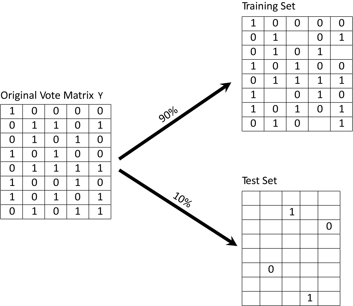
Figure 1 An illustration of our out-of-sample validation strategy with
 $N = 8$
actors and
$N = 8$
actors and
 $J = 5$
votes. Cells are randomly sampled to be in the test set.
$J = 5$
votes. Cells are randomly sampled to be in the test set.
Below, we implement two versions of this cell hold-out strategy to perform out-of-sample validation of ideal point models. The first approach is the simple train-test split we described above: one training sample is used to fit the model with 90% of the cells observed and a performance is evaluated on a test sample with the 10% of cells that were randomly held out. A second strategy is a cross-validation approach where we randomly divide all the cells into 10 groups and treat each of the 10 groups as a test sample in 10 different model fits. For each of these 10 model fits, we use the other 9 nontest groups as the training sample.Footnote 7 This second approach uses all of the data to estimate out-of-sample performance, since each cell appears exactly once in a test sample.Footnote 8
We show in a small simulation study, reported in Figure 4 in Online Appendix C, that the proposed strategy can accurately recover the true dimensionality of the data-generating process with datasets similar in size to those used in this paper.
In terms of identifying the most appropriate number of dimensions, our approach is an application of model selection from statistics and machine learning. We treat each possible dimension D as a separate model and identify the best model based on optimizing a statistic (Hastie et al. Reference Hastie, Tibshirani and Friedman2009). In our case, that statistic is hold-out accuracy, but we could have also made a case for using other well-established model-selection criteria such as AIC (Akaike Reference Akaike1973), BIC (Schwarz Reference Schwarz1978), etc. We have chosen hold-out accuracy, because it is both substantively more interpretable (how much constraint?) and closer to the original notion of constraint put forward in Converse (Reference Converse and Apter1964). Our substantive conclusions are not sensitive to this choice, as we document in Online Appendix E.
Political scientists have previously sought to validate ideal point models in a variety of ways. The most common strategy has been to focus entirely on in-sample measures of fit (i.e., without a hold-out sample). For example, in their work on congressional roll-call voting, Poole and Rosenthal (Reference Poole and Rosenthal1997) report that in-sample accuracy does not increase beyond two dimensions. Jessee (Reference Jessee2009) presents data supporting the same conclusion for survey respondents.
3.3 Estimating Ideal Point Models
Our proposed cross-validation approach requires refitting a multidimensional ideal point model on each dataset 10 separate times. To do this quickly while allowing for large amounts of missing data (due to item nonresponse), we wrote software based largely on the formulas of Imai, Lo, and Olmsted (Reference Imai, Lo and Olmsted2016).Footnote
9
It is described in detail in Online Appendix A and is available online.Footnote
10
 $^{,}$
Footnote
11
Also in Online Appendix B, we show that our one-dimensional ideal point estimates are highly correlated with one-dimensional DW-NOMINATE scores (
$^{,}$
Footnote
11
Also in Online Appendix B, we show that our one-dimensional ideal point estimates are highly correlated with one-dimensional DW-NOMINATE scores (
 $r = 0.97$
) for members of Congress (Poole and Rosenthal Reference Poole and Rosenthal1997) and Shor–McCarty scores (
$r = 0.97$
) for members of Congress (Poole and Rosenthal Reference Poole and Rosenthal1997) and Shor–McCarty scores (
 $r = 0.86$
) for state legislators (Shor and McCarty Reference Shor and McCarty2011).
$r = 0.86$
) for state legislators (Shor and McCarty Reference Shor and McCarty2011).
4 Data Sources
We use several sources of data to evaluate the performance of ideal point models. These datasets are drawn from typical uses in the literature on scaling and cover both politicians and the mass public. For survey questions with more than two ordered response options, we binarize the answers by classifying whether the answer is greater than or equal to the mean. Online Appendix D further describes the variables used in the analysis.
4.1 Senate Voting Data
As a benchmark, we use roll-call votes from the 109th Senate (2005–2007). These data are included in the R package pscl and contain 102 actors voting on 645 roll calls. About 4% of the roll-call matrix is missing.
4.2 NPAT
As a source of survey data among elites, we use data from Project Votesmart’s National Political Courage Test, formerly known as the National Political Awareness Test (NPAT). The NPAT is a survey that candidates take. The goal of the survey is to have candidates publicly commit to positions before they are elected. For political scientists, the data are useful, because they provide survey responses to similar questions across institutions. As such, one prominent use of the NPAT data is to place legislators from different states on a common ideological scale (Shor and McCarty Reference Shor and McCarty2011).
While there are some standardized questions, question wordings often change over time and across states, requiring researchers to merge together similar questions. The full matrix we observe has 12,794 rows and 225 columns. Unlike the roll-call data, however, there is a high degree of missingness: 79% of the response matrix is missing.
4.3 Paired Survey of State Legislators and the Public
We additionally use Broockman’s (Reference Broockman2016) survey of sitting state legislators. This survey contains responses from 225 state legislators on 31 policy questions. Question topics include Medicare, immigration, gun control, tax policy, gay marriage, and medical marijuana, among others. Only about 5% of the response matrix is missing. Additionally, we use a paired survey of the public that is also reported in Broockman (Reference Broockman2016). A subset of the questions are identical to those asked of state legislators. We only use the first wave of the survey, in which there are 997 respondents and no missing data.
4.4 2012 ANES
We use questions from the 2012 American National Election Studies Time Series File, drawn from the replication material of Hill and Tausanovitch (Reference Hill and Tausanovitch2015). There are 2,054 respondents and 28 questions. These questions cover a broad swath of politically salient topics, including health insurance, affirmative action, defense spending, immigration, welfare, and LGBT rights, as well as more generic questions about the role of government. About 10% of the response matrix is missing. We also use various subsets of the American National Election Study (ANES) to investigate heterogeneity in the public.
4.5 2012 CCES Paired Roll Call Votes
Finally, we use data from the 2012 Cooperative Congressional Election Survey. In particular, we focus on the “roll-call” questions, where respondents are asked how they would vote on a series of bills that Congress also voted on. These data have been used to jointly scale Congress and the public (Bafumi and Herron Reference Bafumi and Herron2010). There are 54,068 respondents, answering 10 such questions on the 2012 CCES. The questions cover bills such as repealing the Affordable Care Act, ending Don’t Ask Don’t Tell, and authorization of the Keystone XL pipeline. Only about 3% of the response matrix is missing.
We also match these survey responses to the corresponding roll-call votes in the Senate. These votes took place in the 111th, 112th, and 113th Congresses. We are able to match nine questions to roll-call votes.Footnote 12 A full list of the votes used for scaling is available in Online Appendix D.
5 Evidence on Dimensionality
This section has two goals: first, to demonstrate the existence of overfitting in higher-dimensional ideal point models; and second, to test for which dimensionality best explains variation in political choices. We focus on two sets of data: the 109th Senate (2005–2007) as a sample of political elites and the 2012 ANES as a sample of the mass public. We estimate the ideal point models for these datasets separately for
 $D \in \{0, 1, \dots , 25\}$
dimensions. A
$D \in \{0, 1, \dots , 25\}$
dimensions. A
 $D = 0$
dimensional model only includes an intercept term for each vote. As a measure of model fit, we focus on the estimated accuracy—i.e., the proportion of responses for which the observed choices are most likely according to the model fit. We use the simple 90/10 training/test split we described above. The difference between the accuracy in the training and test sets conveys the degree to which overfitting occurs at that dimensionality.
$D = 0$
dimensional model only includes an intercept term for each vote. As a measure of model fit, we focus on the estimated accuracy—i.e., the proportion of responses for which the observed choices are most likely according to the model fit. We use the simple 90/10 training/test split we described above. The difference between the accuracy in the training and test sets conveys the degree to which overfitting occurs at that dimensionality.
Figure 2 displays the results. For both samples, overfitting occurs within a few dimensions, suggesting that there is actually quite a bit of harm in attempting to model idiosyncrasy with additional dimensions. In the public, statistically significant overfitting occurs even after using just one dimension. In an effort to accommodate a low-dimensional structure model of policy preferences, the fitted model starts to find connections between idiosyncratic preferences that do not generalize beyond the training data. When these connections are applied to the data in the test set, the model is overconfident in its ability to explain idiosyncratic responses that are actually impossible to predict—resulting in a decrease in accuracy relative to the training set. It is clear from this figure that it would be a mistake to compute accuracy only using the training set, since doing so overestimates the generalizability of the model.
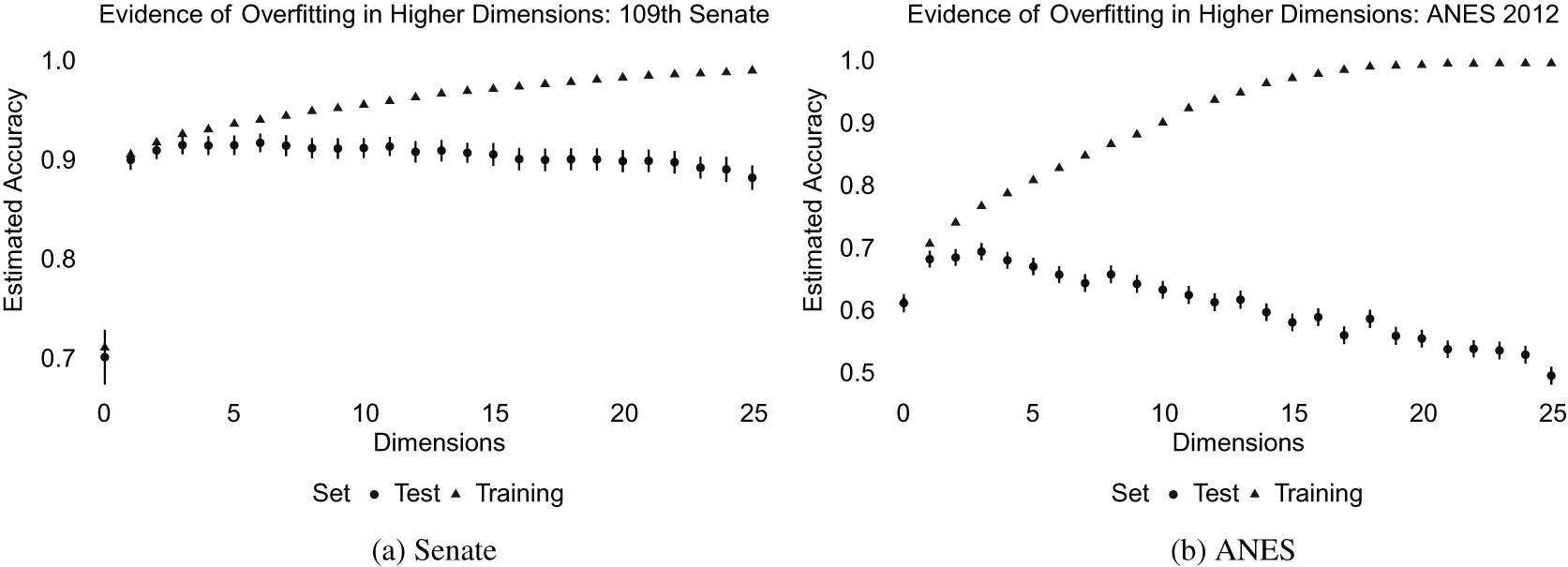
Figure 2 Estimated accuracy within the training and test sets for models fit with latent dimensions
 $D \in \{0, 1, \dots , 25\}$
. Model fit deteriorates after three dimensions for the Senate data and after one dimension for the ANES data. Error bars show 95% confidence intervals, clustered at the respondent level.
$D \in \{0, 1, \dots , 25\}$
. Model fit deteriorates after three dimensions for the Senate data and after one dimension for the ANES data. Error bars show 95% confidence intervals, clustered at the respondent level.
The conclusion from these figures is that the best-fitting model is very low dimensional for both samples. In the public, model fit decreases beyond a single dimension. In the Senate, a one-dimensional model is statistically no worse than any other model. In contrast to the conjectures offered in the literature on political attitudes, the overfitting problem is much more severe in the ANES than in the Senate. For both samples, we can confidently conclude that a one-dimensional model is the most reasonable model.Footnote 13
It might seem possible that these results are a property of the statistical model being applied, rather than a feature of the political actors in these datasets.Footnote 14 However, when these same ideal point models are applied to, say, ratings of movies on Netflix written by movie-watchers, the negative consequences of overfitting do not present themselves until after 30 or 60 dimensions of movie preferences are assumed (Salakhutdinov and Mnih Reference Salakhutdinov and Mnih2008).Footnote 15 It is hard to interpret overfitting results in political data as artifacts of the statistical model being used when those same models can uncover higher dimensions of latent structure in other choice settings. As a whole, the public appears to discriminate over many more attributes when making entertainment choices than when answering questions about politics and policy. This fact should not be too surprising, given that the parties neatly organize policies into two competing bundles. The entertainment market is much more fragmented.
6 Evidence on Constraint
Using the same framework, we now turn to a systematic investigation of ideological constraint. As noted above, we conceptualize constraint as how much better we can predict one set of policy opinions if we know another set of policy opinions, compared to an appropriately chosen null model. In the context of the item-response theory model, this corresponds to a comparison of the performance of an ideal point model, which allows responses to vary depending on an actor’s ideal point, to an intercept-only model, in which predicted responses do not depend on the actor’s ideal point. In the extreme case of no constraint, the predictive performance will be identical, and the difference between a one-dimensional model and an intercept-only model will be negligible. At the other extreme of perfect constraint, a model that includes ideal points will dramatically improve upon the intercept-only model.
The literature suggests that we should expect higher levels of constraint among politicians than among the mass public. We use a number of data sources from both of these populations, which enables a direct test of this hypothesis and allows us to estimate just how much more constrained politicians are than citizens. Our analysis is a “difference-in-differences” approach that compares the improvement in predictive performance among politicians to the improvement among the public. We are, therefore, interested in higher-precision estimates of predictive performance, so we turn to 10-fold cross-validation as outlined in Section 3.
For each dataset, we estimate models with
 $D \in \{0, \dots , 5\}$
dimensions, 10 times each, holding out a 10% sample each time to be used as a test set. For each holdout response, we calculate the likelihood, given the estimated model parameters, of the observed response, and classify its accuracy based on whether the likelihood is greater than
$D \in \{0, \dots , 5\}$
dimensions, 10 times each, holding out a 10% sample each time to be used as a test set. For each holdout response, we calculate the likelihood, given the estimated model parameters, of the observed response, and classify its accuracy based on whether the likelihood is greater than
 $0.5$
. We then calculate the average accuracy across all holdout responses for each model. Given the results in the previous section indicating that responses are best described as one-dimensional, our key measure of constraint is the increase in accuracy moving from the
$0.5$
. We then calculate the average accuracy across all holdout responses for each model. Given the results in the previous section indicating that responses are best described as one-dimensional, our key measure of constraint is the increase in accuracy moving from the
 $D=0$
intercept-only model to the
$D=0$
intercept-only model to the
 $D=1$
one-dimensional model.Footnote
16
$D=1$
one-dimensional model.Footnote
16
6.1 Constraint Among Elites and the Public
The main results are shown in Figure 3. The left-hand panel plots the average cross-validation accuracy for each dataset. The right-hand panel plots the increase in accuracy for
 $D \in \{1, \dots , 5\}$
compared to the intercept-only model.
$D \in \{1, \dots , 5\}$
compared to the intercept-only model.
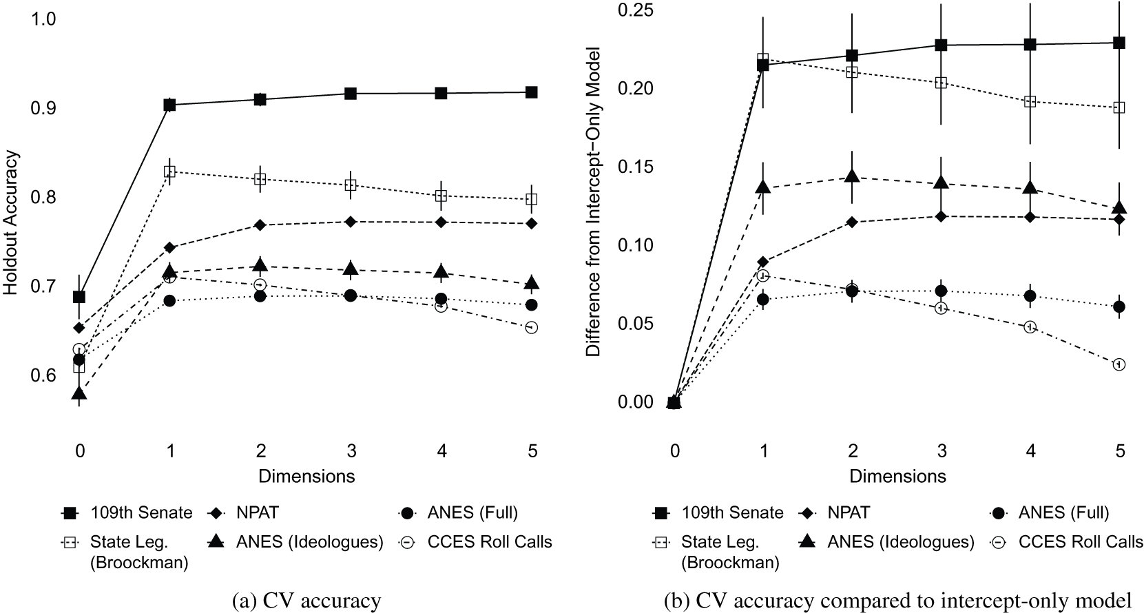
Figure 3 (Left) Cross-validation accuracy for models up to five dimensions. (Right) Increase in percent of accurately classified votes compared to an intercept-only model. Error bars show 95% confidence intervals, clustered at the respondent level.
Beginning at the top of the figures, the solid squares show the cross-validation accuracy of ideal point models for roll-call votes in the 109th Senate. The left-hand panel shows that nearly 90% of votes are correctly classified by a one-dimensional ideal point model. The right-hand panel shows that this is about a 20 percentage point increase over the intercept-only model. As discussed in the previous section, there is little additional gain in accuracy for the Senate data moving beyond a single dimension, though the out of sample performance does not degrade either.
Next, the hollow square shows the results when applied to data from Broockman’s (Reference Broockman2016) survey of state legislators. A one-dimensional model can accurately classify roughly 83% of responses. Again, this is an increase of over 20% percentage points compared to the intercept-only model. Here, the performance of the model begins to decay once we estimate more than a single dimension. This result again underscores the unidimensionality of political constraint among political elites.
The one-dimensional model performs less well when applied to the NPAT data, as illustrated by the solid diamonds. A one-dimensional model correctly classifies only about 75% of responses—an increase of less than 10 percentage points over the intercept-only model. This increase is less than half of the gain achieved with the other two sources of elite data. There is a mild increase in accuracy associated with a second dimension, though the increase is only about 2 percentage points.Footnote 17
Notwithstanding the NPAT results, the picture that emerges from this exercise confirms the conventional wisdom that politicians—at both the national and state level—are highly constrained in their preferences. Two-thirds of inexplicable votes under the null model are now predictable due to the inclusion of a one-dimensional ideal point.
Such a dramatic increase does not hold for the public. As noted above, we use data from the 2012 ANES and CCES. The nature of the questions included differs between these sources. For the ANES, the questions are typical of public opinion research. The CCES questions, however, ask respondents how they would vote on particular roll-call votes that were actually voted on in Congress. Despite the differences in question format, our substantive conclusions are identical for both datasets.
Consider the solid circles in Figure 3, which correspond to the full sample of ANES respondents. The left-hand side shows that an intercept-only model correctly classifies about 62% of responses. Adding a one-dimensional ideal point increases this classification accuracy to about 69%. Similarly, an intercept-only model correctly classifies about 63% of CCES roll-call responses, compared to 71% accuracy for the one-dimensional model. In both cases, additional dimensions do not increase the performance of the models and, in the case of the CCES, degrade the performance.
These results suggest that classification accuracy increases by about 12% in a one-dimensional model compared to an intercept-only model.Footnote 18 Despite using a different methodology, Lauderdale et al. (Reference Lauderdale, Hanretty and Vivyan2018) come to a similar conclusion; they report that about one-seventh of the variation in survey responses can be explained by a one-dimensional ideal point, while the rest they attribute to idiosyncratic or higher-dimensional preferences.
Overall, we take these results to mean that there is some constraint in the public, but the relationship between the estimated ideal points and the survey responses is much noisier among the public than it is among elites. For the ANES and CCES, a one-dimensional ideal point model only increases classification accuracy by about 7 or 8 percentage points compared to an appropriate null model. Only about 20% of unpredictable votes under the null model are now predictable using ideal point models. This number pales in comparison to the 67% of inexplicable-turned-predictable votes for the national and state political elites.
6.2 Investigating Heterogeneity in the Public
Of course, there is heterogeneity in the level of constraint in the public, and the overall results may mask constraint among a meaningful subset of the public. As a preliminary test of this possibility, we rerun the ANES analysis after subsetting to people who say self-identify as ideological (i.e., answer 1, 2, 6, or 7 on a 7-point ideology scale). This group of people is likely to have better-formed opinions about political issues and to perceive a common policy space, implying that we may observe more constraint in this population. These results are shown in the solid triangles in Figure 3. As expected, ideal point models have higher accuracy among this subset than among the ANES respondents as a whole. A one-dimensional model can correctly classify 73% of responses among this subset, compared to only 60% that are correctly classified by the intercept-only model. The right-hand panel also shows that the absolute increase in accuracy is actually larger than the increase for the NPAT. Still, compared to the Senate roll-call votes or the state legislator survey, the increase in accuracy is relatively small, again highlighting the higher level of constraint among elites than the public.
A fuller picture is presented in Figure 4, which shows the average increase in classification accuracy for each respondent from a one-dimensional model, relative to the intercept-only model, across a number of political and sociodemographic variables. The black points show the results when the cross-validation procedure is run on the full dataset, while the gray points show results when it is run on each subset separately.Footnote 19 The political variables include whether the respondent was contacted by or donated to a campaign, the respondent’s self-report ideology, party identification, and whether the respondent correctly places the Democratic Party to the left of the Republican Party on an ideology scale (Freeder et al. Reference Freeder, Lenz and Turney2019). The socioeconomic variables include age, education, gender, family income, and race.
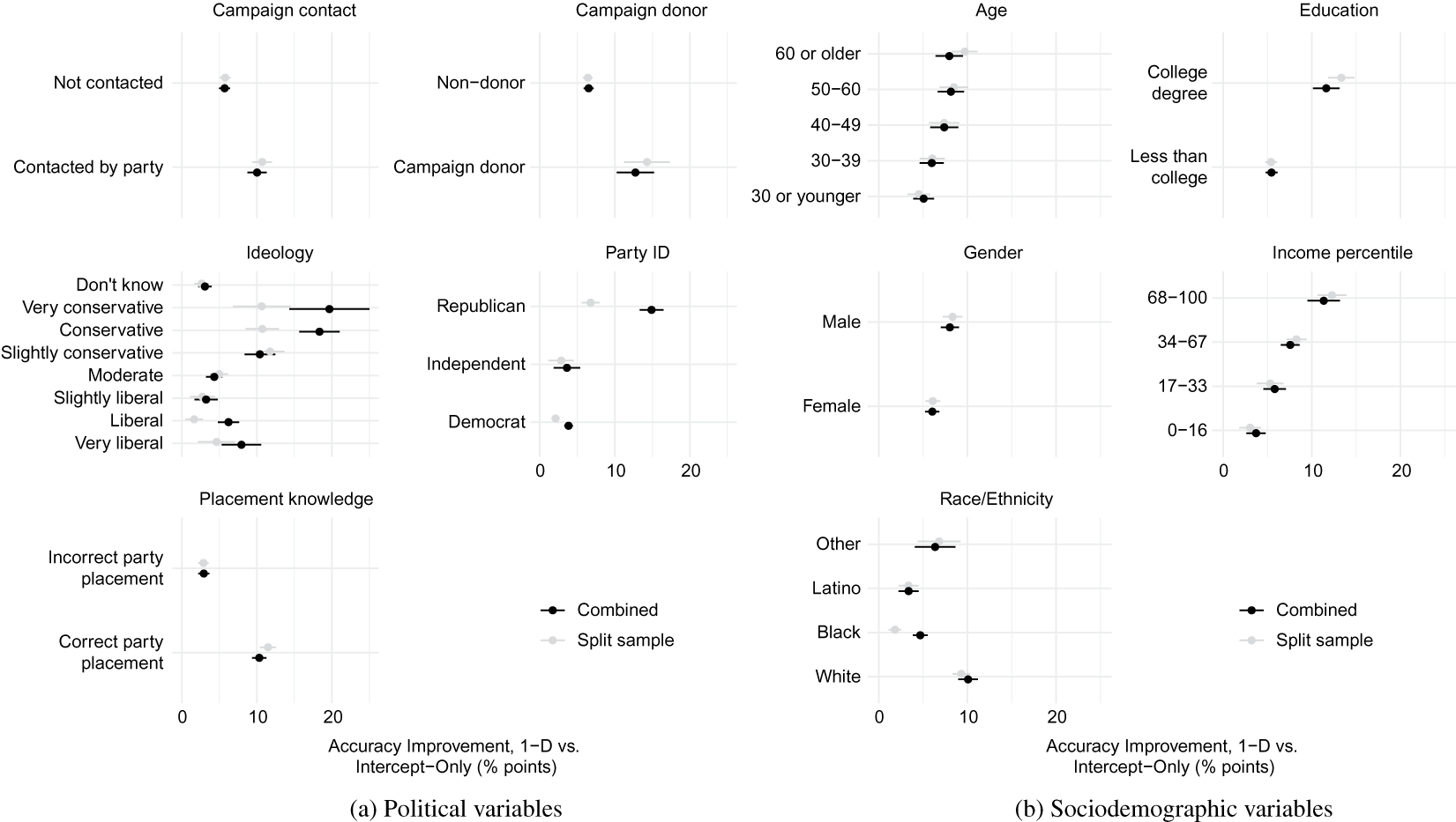
Figure 4 Constraint among subsets of the public. The points show the average respondent-level increase in classification accuracy obtained by a one-dimensional ideal point model relative to the intercept-only model. Bars show 95% confidence intervals. The black points show results when all respondents are used in the cross-validation procedure, while the gray points show results when cross-validation is performed on each subset separately. “Placement knowledge” refers to whether respondents place the Democratic Party to the left of the Republican Party on a 7-point ideology scale (Freeder et al. Reference Freeder, Lenz and Turney2019).
The results suggest that there is indeed heterogeneity in the public. Broadly, we find significantly more constraint among conservatives than liberals, Republicans than Democrats, and those who are more knowledgeable and engaged with politics. Similarly, we find greater constraint among people who are older, more highly educated, and richer.
Nonetheless, only in a few subgroups—namely, conservatives and Republicans—does the increase in out-of-sample predictive accuracy come close to the increase seen among politicians.Footnote 20 For the vast majority of subgroups we study, a one-dimensional ideal point model does help predict responses better than an intercept-only model, but the gains are very modest in comparison to politicians.
6.3 Explaining the Public-Politician Divide
Our results thus far suggest that ideal point estimates extract relatively little information from survey responses of the mass public—at least when compared to politicians. Our preferred interpretation is that the public simply has a lower degree of ideological constraint than political elites.
But there are at least three alternative explanations that we probe in this section. The first is that surveys and roll-call votes are very different environments. Survey respondents face few incentives to thoughtfully consider their responses before answering, which may lead to an increased amount of noise in their responses. In contrast, roll-call votes in Congress are “real-world” actions that provide obvious incentives to vote in particular ways.
Second, even if one grants that survey respondents reveal genuine preferences, one might object on the grounds that the set of topics covered in the datasets are not the same. If roll-call votes in Congress are simply better tools for discriminating ideology than survey questions, we would overestimate the degree of constraint in Congress relative to the public.
Third, given the results of the previous section showing some evidence of heterogeneity in the public, it could be that the increased constraint among politicians is simply explained by the unrepresentative demographics of politicians.
To assess the plausibility of these hypotheses, we take advantage of two paired datasets, in which politicians and the public respond to identical questions. Recall that the CCES questions correspond to roll-call votes that were recently held in Congress. This feature allows us to compare the performance of scaling methods using the exact set of issues in Congress and on the CCES. If differing agendas are the cause of the divergent results above, then we should see the divergence in constraint between the public and political elites shrinks when restricting ourselves to a common agenda. Additionally, we can run the analysis on both the full set of CCES respondents as well as a subset that is selected to mirror—to the extent possible—the demographics of the Senate.Footnote 21 If either the agenda or demographics explain our results, then this sample should show a similar degree of constraint as Senate roll-call voting.
The left-hand panel of Figure 5 shows the roll-call measures for the Senate and the CCES, for both the full sample and the sample matched to Senate demographics. Despite including only 8 roll-call votes in the Senate, a one-dimensional model accurately classifies nearly 90% of votes—compared to less than 60 in the intercept-only model. In contrast, the accuracy among the public on the same questions goes from 63% to 71% in the full sample. The CCES sample that is demographically matched is somewhere in between, with accuracy increasing from 63% in the intercept-only model to 79% in the one-dimensional model. This finding provides confirmation of the prior result that there is heterogeneity in the level of constraint across the public. Still, even among this group of respondents who are demographically similar to Senators, their survey responses are less predictable than Senators’ roll-call votes. Some, but not all, of the increased constraint seen among politicians can be explained by their demographics.
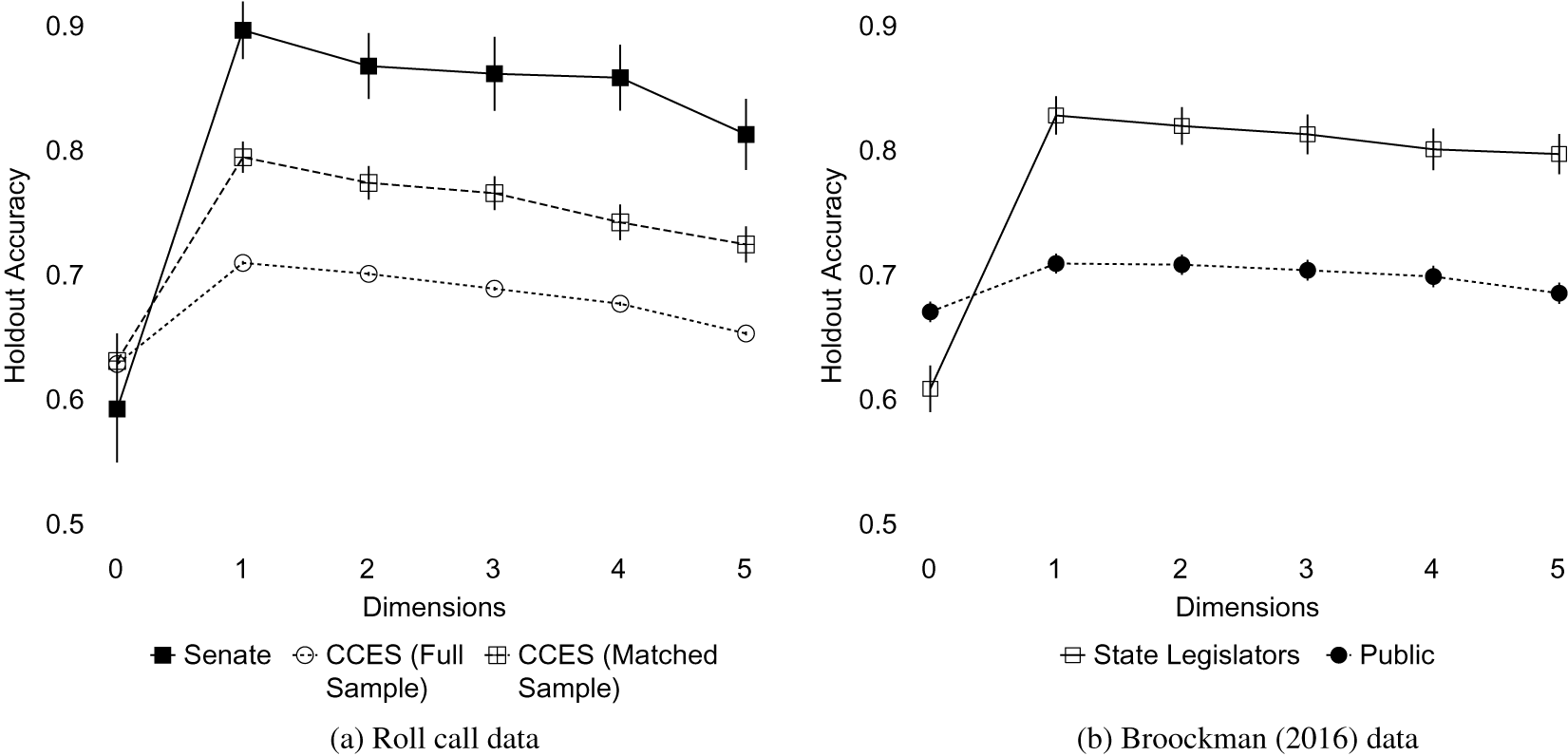
Figure 5 Comparison of cross-validation accuracy in the public and among elites, holding the survey items constant. Error bars show 95% confidence intervals, clustered at the respondent level. Even with common agendas and incentives, politicians exhibit a higher degree of constraint than the public.
Finally, returning now to the first objection, if there are different incentives created by the roll-call context, we might still observe differences. To probe this question, we take advantage of a parallel survey of the mass public that Broockman (Reference Broockman2016) conducted along with the state legislator survey. Here, legislators’ responses were anonymous, so the incentive structure inherent to survey-taking is the same for both the mass public and elites.
The results are shown in the right-hand panel of Figure 5. They tell an even more stark story when the survey context is held fixed: politicians’ responses are quite predictable, while the public’s are not. This result suggests that it is not the use of surveys per se that is driving the difference between politicians and the public.
These results suggest that the driving force behind the divergent performance of ideal point models in the public relative to elites is primarily the differing levels of constraint of politicians as politicians—not a different agenda, different incentives faced by actors operating in public and private, nor the demographic characteristics of politicians, although this last element does play a part.
7 Conclusion
The main contributions of this paper are twofold. First, we formalize the notions of multidimensionality and constraint in a theory of political choices based on the canonical spatial voting model. From this discussion, we highlight observable implications that relate to the dimensionality of political conflict and the level of constraint in a given population. Second, we propose an out-of-sample validation strategy to evaluate empirically the structure of political choices in a broad range of data sources. We focus on out-of-sample validation both for substantive reasons—“constraint” naturally refers to how well a person’s opinion on one set of issues predicts her opinion on others—and for methodological reasons—in-sample measures of model fit are biased toward finding more dimensions and more constraint than are actually present.
The importance of out-of-sample validation is apparent from our empirical results: we find that ideal point models that contain more than a single dimension are counterproductive. Political choices in the United States, whether by survey respondents or Senators, are best approximated as one-dimensional.
In the Senate, this result is unsurprising. However, conventional wisdom holds that political opinions among the mass public may be more nuanced than a single left–right scale, implying that a higher-dimensional structure may exist. We find no evidence of such a higher-dimensional structure. If anything, moving beyond a single dimension tends to produce worse inferences in the public than among politicians due to overfitting.
Next, we turn to the issue of constraint. We operationalize constraint as the increase in predictive performance that can be achieved by a model that explicitly incorporates an actor’s ideal point, relative to a model that does not. Using cross-validation, we show that political elites are highly constrained, while members of the mass public are relatively unconstrained. About two-third of the choices among politicians that cannot be predicted by an intercept-only model can be predicted when we estimate a model with a one-dimensional ideal point. In contrast, only about 20% of survey responses in the mass public that are unpredictable in an intercept-only model become predictable when the model includes an ideal point.
Using a series of paired datasets, we show that this difference in predictive performance cannot be attributed to the survey instrument, nor to differences in the agenda, nor to differing incentives faced by politicians and regular citizens. The most likely explanation, in our view, is the most simple: politicians organize politics in a more systematic way than most citizens. There is also evidence of heterogeneity in the public. Ideal point models fare better at predicting individual issue attitudes among people who look demographically more similar to politicians.
Substantively, these results suggest caution when applying ideal point models to survey responses from the mass public. While the public is best approximated as having one-dimensional ideal points, this ideal point does not predict attitudes on any given issue particularly well. In the public, it appears that idiosyncratic, rather than ideological, preferences explain the majority of voter attitudes. Our work suggests that scholars of public opinion should pay heed to both ideological and idiosyncratic portions of policy attitudes.
Acknowledgments
For helpful discussions and comments, we thank Adam Bonica, David Broockman, Justin Grimmer, Andy Hall, and Jonathan Rodden. We are especially grateful to Adam Bonica for sharing the NPAT data. We also thank the participants of the Political Economy Breakfast and the Workshop for Empirical American Politics Research at Stanford.
Data Availability Statement
An R package for implementing the MultiScale algorithm is available at https://github.com/matthewtyler/MultiScale. Replication code for this article has been published in Code Ocean, a computational reproducibility platform that enables users to run the code and can be viewed interactively at Tyler and Marble (Reference Tyler and Marble2020a) at https://doi.org/10.24433/CO.3851328.v1. A preservation copy of the same code and data can also be accessed via Dataverse at Tyler and Marble (Reference Tyler and Marble2020b) at https://doi.org/10.7910/DVN/SWZUUE.
Supplementary Material
For supplementary material accompanying this paper, please visit https://doi.org/10.1017/pan.2021.3.


