2 The Limitations of Existing Methods

Researchers have a number of tools to assess attentiveness on self-administered surveys. Among those most often used are IMCs or screener questions (e.g., Berinsky et al. Reference Berinsky, Margolis and Sances2014; Oppenheimer, Meyvis, and Davidenko Reference Oppenheimer, Meyvis and Davidenko2009). These questions mirror other regular survey questions in length and format but ask the respondent to ignore the standard response format and instead confirm they have read the question by providing specific answers. Researchers can then analyze participants’ responses to this question to identify those who carefully read and followed the hidden instruction. However, introducing screener questions comes at a cost. Scholars recommend the inclusion of multiple such questions to measure attentiveness accurately (Berinsky et al. Reference Berinsky, Margolis, Sances and Warshaw2019), which means increased questionnaire length and completion time. This strategy might also result in greater respondent fatigue, and thus influence responses to latter questions (Alvarez et al. Reference Alvarez, Atkeson, Levin and Li2019). Moreover, there are no standardized screener questions, and question length can be a powerful predictor of a respondent’s likelihood to fail the screener (Anduiza and Galais Reference Anduiza and Galais2016).

An unobtrusive alternative is the use of survey response time to assess respondent attentiveness. Response time (or response latency) is the amount of time a respondent takes to answer a question, measured as the number of seconds between the respondent’s first click onto a page and last click leaving a page. Response times are an example of paradata, like mouse-clicking or eye-tracking patterns, that provide insight into how respondents are taking surveys (Yan and Olson Reference Yan, Olson and Kreuter2013). Response time correlates with other proxies of response quality, such as self-reported effort (Wise and Kong Reference Wise and Kong2005), attention to detail (Börger Reference Börger2016), response consistency throughout the survey (Wood et al. Reference Wood, Harms, Lowman and DeSimone2017), straight-lining (Zhang and Conrad Reference Zhang and Conrad2014), and susceptibility to survey design effects (Malhotra Reference Malhotra2008).

Yet how to effectively use response-time data remains an active area of research. As Fazio (Reference Fazio1990, p. 89) writes, “there may be nothing scientifically less meaningful than the simple observation that subjects responded in X milliseconds.” Making these data meaningful involves three steps. First, researchers must decide whether to only use response-time indicators for some survey items, or to aggregate all items together into one response-time metric. Second, they must decide which response times represent markedly fast and slow answers, and determine cutoff thresholds for categorization. Finally, researchers must determine how respondents’ response-time metric maps onto the latent measure of survey-taking behavior that researchers wish to examine. For example, are slow respondents distracted or confused?

To address the first issue of how to aggregate response-time patterns across questions, many studies assess response time globally (Malhotra Reference Malhotra2008), looking at the raw total response time for survey completion. Other researchers develop attentiveness measures that look at single question response times (Zandt Reference Zandt, Pashler and Wixted2002) or compare response times within or between specific modules (Vandenplas, Beullens, and Loosveldt Reference Vandenplas, Beullens and Loosveldt2019) and experimental conditions (Fazio Reference Fazio1990). From there, researchers will often calculate an aggregate score that indicates the proportion of survey questions which the respondent answered above or below a time threshold (see, e.g., Barge and Gehlbach Reference Barge and Gehlbach2012; Greszki, Meyer, and Schoen Reference Greszki, Meyer and Schoen2015; Wise and Kong Reference Wise and Kong2005; Yan et al. Reference Yan, Ryan, Becker and Smith2015).

However, there is no consensus as to what such a response-time threshold should look like; whether it should be a common threshold, or dependent on the question content or the distribution of response times (Huang et al. Reference Huang, Curran, Keeney, Poposki and DeShon2012; Kong, Wise, and Bhola Reference Kong, Wise and Bhola2007). Even if researchers do not pick a threshold and use the raw data, they still must decide whether attentiveness is increasing or decreasing with response times, or if the relationship is curvilinear.

This brings us to our third conceptual decision. Researchers need to determine what it means substantively when respondents rush through or drag throughout surveys. Here, researchers are divided in their interpretation of response time. One cohort of scholars argue that response time is a measure of attitude accessibility (Huckfeldt et al. Reference Huckfeldt, Levine, Morgan and Sprague1999; Johnson Reference Johnson2004; Mulligan et al. Reference Mulligan, Grant, Mockabee and Monson2003) or the clarity of the survey instrument itself (Bassili and Scott Reference Bassili and Scott1996; Olson and Smyth Reference Olson and Smyth2015). For these researchers, long response times indicate either that respondents are struggling to connect attitudes to questions, or that the survey instrument is impenetrable. Notably, these scholars largely focus on response time in interviewer-administered surveys (face-to-face or phone surveys), where respondents are less able to multitask than with self-administered web surveys.

Researchers examining response time in web-based surveys, however, are usually concerned with the fast end of the spectrum, suggesting that when respondents answer very quickly, they have not taken enough time to understand the question and provide an accurate answer. Instead, they are satisficing (Callegaro et al. Reference Callegaro, Yang, Bhola, Dillman and Chin2009; Greszki et al. Reference Greszki, Meyer and Schoen2015). The assumption here is that rushing respondents are inattentive. We join these scholars in arguing that response times are indeed a clear indicator of attentiveness, rather than respondent comprehension. Our validation exercises show that this is likely the case. While we generally agree that response time can be an indicator of respondent attentiveness, we argue that the relationship between the two variables is not strictly monotonic. In particular, respondents’ ability to multitask and propensity to be distracted in web-based surveys means that very long response times, not just particularly short ones, can also be indicative of inattentiveness.

To highlight these points, we visualize trends in actual response-time behavior. We present data on response time from a survey fielded in 2016 using Survey Sampling International (SSI)Footnote ² to illustrate response-time fluctuation throughout a survey, and the degree to which different questions provide vastly different amounts of information about survey-taking behavior.

The first important trend that emerges from the data is that global measures of response time obscure important within-respondent variation. Response-time behavior often fluctuates throughout the course of a single survey. Figure 1 shows the per-question response time for two illustrative survey-takers. Both respondents have similar average and global response times; the difference between their aggregate response times is less than a one-hundredth of a standard deviation. Yet they behave very differently. One respondent takes considerably more time to answer complex ranking and grid questions. The other spends significantly more time on basic factual questions about the respondent’s gender, education, religion, and ideological affinity. These important differences are concealed under any approach that looks at aggregated response times.

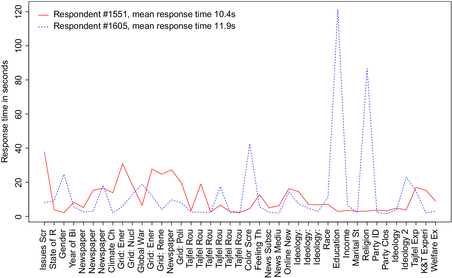
Figure 1 Average response time conceals important cross-question variation. This figure shows the per-question response time for two respondents who have similar average question and global survey response times. Respondent #1551 has an average question response time of 10.4 s, 1.5 s less than Respondent #1613, a difference of less than a one-hundredth of a standard deviation. Despite similar average response times, these two respondents behave very differently. Respondent #1551 spends more time on complex grid and ranking questions (Climate Ch and Grid), whereas Respondent #1605 dwells on questions that ask about the respondent’s gender, favorite color, educational background, religion, and ideology.

Moreover, such an approach inherently assumes that each question provides the researcher with the same amount of information about the respondent’s overall attentiveness. This assumption seems problematic. When the question is short, the answering process is straightforward. Both attentive and inattentive respondents answer quickly. It is when respondents encounter longer and more complex questions that actually require respondents to process the question setup and think carefully about their answers that we should expect response times to be a good indicator of a survey-taker’s attentiveness. To illustrate, Figure 2 shows boxplots for the response times for all questions in our 2016 survey. The distributions highlight that there is a great deal of variation in the amount of information contained in each question. Importantly, for some questions, most respondents are relatively fast. On other questions, however, there are respondents who are both much faster and much slower than the middle 50% of the response times. These latter types of questions are likely to offer us more information on respondent attentiveness than the former type. Figure 2 clearly suggests that it is in more complicated questions, such as experiments (Tajfel and KT Experiment), that we can find the most response-time variability.

Figure 2 Questions with larger response-time variation provide more information on attentiveness. This figure displays a boxplot for each question contained in our data with the distribution of response time across respondents. We can see that for some questions, for example, Party ID, the bulk of the respondents are relatively fast. On other questions, however, there are respondents who are both much faster and much slower than the middle 50% of the response times (e.g., Grid: Energy Tax). These latter types of questions are likely to better distinguish attentive from inattentive respondents than the former type.

Figures 1 and 2 also highlight a final important point: some respondents can take a very long time to complete survey questions. The existing literature often overlooks this type of slow respondent. Focusing primarily on “rushing” respondents, existing measures assume that extremely short response times are indicative of satisficing. That is, past a certain extremely short threshold time, response times do not provide much information about attentiveness or satisficing. Yet there is a substantial amount of variation to explore at the slower end of the distribution. Simply put, if rushing were the only deviation from typical survey-taking behavior, we would see more outliers toward the fast end of the scale, and fewer toward the slow end. Instead, modeling respondent behavior on self-administered online surveys needs to take into account Internet browsing behavior, which may include switching between different tabs and engaging in several activities at the same time. Using response time as a proxy for respondent attentiveness could therefore benefit empirically from incorporating all respondent data, and theoretically from introducing slow respondents as a third category of inattentive respondents.

3 A New Approach to Estimating Response Time

The first step in our approach lies in conceptualizing attentiveness as a latent variable.Footnote ³ It is not a single observable variable but a multidimensional concept that incorporates how closely respondents read questions, how deeply they understand the text, how thoughtfully they answer the questions, and how well they are able to remember survey content over several pages of questions. None of these metrics, however, can be directly observed and recorded by the researcher; thus, researchers rely on observable behaviors to proxy for respondent attentiveness. To translate response-time paradata to attentiveness, we introduce RTAC to proxy for attentiveness.

3.2 The Empirical Framework

Thus, conceptually, there are not only different types of inattentive respondents, but also respondents who take surveys at similar paces might be different. Response time, as a measure of attentiveness, is therefore a multidimensional concept. The average response time across all questions tells us one thing, but the variation in how long respondents spend on each question tells us another crucial piece of information about attentiveness. Figure A.2 in the Online Appendix provides empirical support for this interpretation, showing that there is a strong and positive correlation between response time and variance for respondents across all questions, suggestive of a different data-generating process for very fast and very slow respondents. RTAC takes both these patterns—average time across all questions, and fluctuations in timers across all questions—into account.

Building on previous research on response time, and attempting to account for some of its short-comings, RTAC needs to perform several specific functions. First, it needs to use all the response-time data in a parsimonious fashion to avoid making arbitrary decisions about which variables to include or exclude. Second, it should include a trifold classification of survey attentiveness to allow for the inclusion of slow respondents and account for nonmonotocity in the relationship between response time and attentiveness. Third, it should provide a disciplined way of identifying who is slow or fast that is based on similarities in response-time behaviors across respondents, rather than subjective cutoff thresholds for response time.

For this, we rely on two methods: PCA, which extracts the maximum amount of variation from the data to provide an optimal low-dimensional representation of the data and captures multiple dimensions of variation (e.g., total time and variation in timing between questions), and EM, which fits a GMM to cluster our response-time data into categories based on underlying similarities in the data. Together, these methods meet the criteria for RTAC expressed above.

Figure 3 provides an overview of the process. After transforming the response-time data to avoid overfitting the clusters of respondent attentiveness, we perform two empirical steps. First, we preprocess the response-time data with PCA to reduce its dimensionality. This reduces the number of dimensions of response time that we need to incorporate into our model from a dimension for each question to a smaller, parsimonious set of uncorrelated dimensions. If we believe that each per-question response-time indicator does not capture wholly different information about how a respondent takes a survey, then PCA will collapse the response-time data into a set of orthogonal dimensions that combine similar features of the data.

Figure 3 Overview of estimation process.

We use the transformed response-time data to cluster respondents into three attentiveness categories. To do this, we use the EM algorithm to estimate membership in a GMM. This type of model assumes that the data at hand are not drawn from the same one distribution, but rather from multiple distinct normal distributions, each with its own parameters (mean and variance). The algorithm then estimates both the shapes of those normal distributions, and calculates the probability that a data point belongs to each of those distributions. Under our theoretical framework, we assume there to be three distinct groups of survey-takers, and each is drawn from a distribution of response times with a distinct mean and variance: fast/inattentive, slow/inattentive, and baseline/attentive. The algorithm we employ therefore calculates the probability that a respondent belongs to one of three clusters, each representing a different type of survey-taking behavior. From here, we explain the methodology in greater detail. Readers who are less interested with the technical details behind the method should skip to Section 3.3.

The first step of our approach is preprocessing: taking high dimensional data—response time for each question—and condensing them such that the data are parsimonious while still capturing sufficient variation to characterize respondents. This focuses our analysis on those parts of the data where we can find the most information about respondents’ survey behavior. As highlighted in Figure 2, many survey questions contain very little information about how long different respondents take to answer the questions (i.e., have low variance), while others are much more discriminating. Therefore, the full matrix of per-question response times is likely to have a high noise to signal ratio. To reduce such noise, researchers might be tempted to subset the data to only those questions with high variance in response times; however, this would require a subjective evaluation of what “high variance” means. We therefore prefer to use PCA to extract the meaningful variance from the data.

PCA transforms highly correlated variables into a smaller set of uncorrelated variables for the purpose of dimension reduction, allowing researchers to use a parsed-down number of variables to represent variation in the original data. By projecting data onto a lower-dimensional space, the PCA algorithm identifies directions in which the data vary. The first principal component contains the most variation, while the second principal component contains the most variation orthogonal to the first component. The process continues until it has projected the data onto a k-dimensional space, where k is the number of variables in the original dataset.

We proceed by performing a PCA on a matrix of logged response timesFootnote ⁵ for each question and each respondent.Footnote ⁶ Often, researchers use PCA to develop an index measure constructed of several correlated measures. For example, if someone wanted to measure ideology using a battery of questions concerning political beliefs, they might run a PCA, extract the first two dimensions, and name them the “economic” and “social” dimensions of opinion. However, we use PCA for a different purpose. We employ PCA to weight the response-time indicators according to how much information each indicator contains about overall response-time behavior. Each variable input to the PCA measures the same thing: how respondents interact with the survey instrument. The PCA extracts the maximum amount of information from that data and provides us with appropriate weights that allow us to glean as much information as possible from response time without having a very sparsely populated dataset. Thus, unlike most PCA users, we are not interested in interpreting what each PCA dimension means.

That said, examining the PCA loadings can help illustrate how the PCA is working in practice. We show the first component’s loadings—i.e., the weights that indicate the relationship between each variable and principal component—in Figure 4. As expected, we observe that longer and more complex questions, including those of two survey experiments (K&T Experiment and Tajfel Experiment), those where respondents had to evaluate their own position on a scale (questions starting with Ideology), and large grid questions (those starting with Grid) are the main variables loading onto the first dimension. These variables therefore contribute to a great deal of the variation contained in the first component. Indeed, we would expect longer and more complex questions to exhibit the greatest amount of variation as attentive respondents will take the time to read a block of text, whereas fast respondents will continue rushing through. In contrast, easy questions that require very little processing and recall, like questions about the respondent’s race, year of birth, and gender, contribute the least amount of the variation to the first component.

Figure 4 Variable loadings on first principal component. This plot shows the degree to which question response times are included in the first component of the PCA, and the complexity (word count) of those questions. Complex questions, including experimental questions (K&T Experiment and Tajfel Round), grid questions (those starting with Grid), and scale questions (those starting with Ideology) contribute the most to the first component.

We confirm this relationship in Figure 4b, showing that there is a positive trend between word count and contribution to the PCA’s first dimension. In plain English, this means that longer questions have the most variation in response time, providing the PCA a good deal of variation with which to work. Longer questions are most informative. However, this does not mean we should only include the first principal component in our analysis. While the first dimension captures variation in response times for long and complex questions, subsequent dimensions capture variation in shorter questions and within-respondent differences across questions (e.g., respondents who take a long time to answer grid questions but are quicker on scale questions). Those dimensions therefore contain meaningful information about survey-taking behavior that should not be discarded, as is often done in response-time aggregation methods.

There are few clear methods for deciding how many components to retain in dimensional reduction. The central question to ask is how much variation is needed to understand the patterns in the data. There is no correct answer to this question; inherent in this decision is a trade-off between capturing variance (retaining more components), and losing parsimony (retaining fewer components). Some researchers rely on the visual examination of a scree plot, which shows the eigenvalues of the principal components, to determine the point at which these eigenvalues level off. We prefer to follow the procedure of examining the proportion of variance explained cumulatively by the principal components, and retain those components that explain 80% of the total variation. In our case, this means retaining the 19 first principal components. We examine the robustness of this decision in Section 3.3, and show empirically in the Online Appendix that estimation becomes stable once about 80% of the variation is used, as well as provide an example of how users can conduct their own robustness checks on PCA.

The PCA weights provide the preprocessed inputs used to assign attentiveness cluster membership for each respondent. Given the latency of respondent attentiveness as a variable, previous work relies on observable outcomes (choice patterns, IMC passage, and response time) to group respondents into different categories of survey attentiveness. Grouping this latent variable into a discrete number of categories allows researchers to have a number of theoretically driven clusters to categorize respondents, providing comparability across surveys with different distributions of respondent attentiveness, and numbers and types of questions.

Clustering algorithms lend themselves particularly well to the task of estimating latent attentiveness. Generally speaking, these unsupervised machine learning techniques can identify similarities in data points and thus group similar data points together. In our case, we use the response-time data weighted by the first 19 principal components as our input data. A clustering algorithm can then group respondents according to similar patterns in their response times, using both response times and their variability within and across respondents. This approach presents a number of advantages over other measurement strategies. First, as an unsupervised machine learning technique, we are not required to make ad hoc decisions about which response times count as slow, baseline, and fast. Previous literature made idiosyncratic decisions about the answer time thresholds that classified as “too fast” (see Kong et al. Reference Kong, Wise and Bhola2007, for a discussion). An unsupervised clustering algorithm does not require such decisions. It groups data points according to their multidimensional characteristics. The researcher can then inspect those groups and ascertain which one is faster or slower. Second, the input data for such algorithms can be multidimensional. In other words, instead of limiting ourselves to just using one data point per respondent, such as the global or average question response time or response time during survey experiments (Harden, Sokhey, and Runge Reference Harden, Sokhey and Runge2019), we are able to retain all the data and use it to estimate the parameters of multivariate normal distributions.

Many methods for clustering exist, with centroid models (e.g., K-Means clustering) and distributional models like GMMs, which are fit with methods like EM, being two main contenders for this task. The K-Means algorithm finds groups by starting with initially random group centers, and then assigns each data point to the group center to which it is closest, improving the clusters in each iteration. This approach suffers from a few drawbacks. First, data points are “hard assigned” to a group; group membership is binary, and researchers are unable to see the probabilistic assignment into a particular group. Second, the underlying models from which these data points are generated are assumed to be centroids and not full distributions. This is problematic for our approach, because theoretically, we think that slow, distracted respondents would have different distributions of response times across questions, rather than simply different means.

GMMs, fit with an EM algorithm, find groups by determining a mixture of normal distributions that best fit the data. More specifically, this model assumes that each group is a Gaussian distribution with a mean and variance–covariance matrix, and each data point has been drawn from the distribution associated with its group. An EM algorithm proceeds iteratively. In the E-step, given the current assignment of data points to groups or distributions (initially done at random), each groups’ distributional parameters are updated. In the M-step, we estimate the posterior probability of group membership given each group’s updated parameters. In other words, the algorithm looks for a better group assignment and reassigns data points to the distributions they are most likely to come from, conditional on the distribution’s updated mean and variance–covariance matrix. The algorithm iterates through this process until it converges, and produces as an output the maximum a posteriori estimate of each respondent’s probability of belonging to each group. This approach presents a number of advantages. First, it allows for three different categories of respondents, each of which behaves very differently in responding to the survey, corresponding to different time distributions. Second, it provides us with a “soft” group assignment that indicates the probability that a respondent belongs to a specific group, rather than a hard assignment that leaves no room for uncertainty. We can thus determine how likely a respondent is to belong to a certain cluster.

In this algorithm, random variable x is the weighted sum of a mixture of K Gaussian distributions or groups. We treat respondent group membership as an unobserved variable z and are then able to calculate the joint distribution of $p(x,z)$ according to the marginal distribution of $p(z)$ . With latent variable z, respondents take a value of 1 if they are assigned to group $z_k$ and a 0 otherwise. Finally, we are also able to calculate the conditional probability of z given x, which allows us to estimate the posterior probability of membership in each of k categories according to the observed x. The EM algorithm also allows us to calculate the responsibility for each observation, which is the probability that each observation fits into each of k categories. These probabilities sum to 1.

Given our theoretical motivation, we model a Gaussian mixture distribution with three distinct Gaussian distributions or groups, using the response-time scores weighted by the first 19 principal components. We find that the algorithm clearly assigns the vast majority of respondents into one of the three categories. Graphic inspection of the EM sorting, available in the Online Appendix, shows that for each cluster, most respondents have a responsibility of either 1 or 0, meaning the algorithm assigns them probabilities of close to 1 or close to 0 of belonging to that group. From there, we hard assign each respondent to the cluster of which he or she is most likely to be a member (i.e., the cluster with the highest posterior responsibility (McLachlan, Lee, and Rathnayake Reference McLachlan, Lee and Rathnayake2019)).Footnote ⁷

We then inspect the group membership assignment more closely. Figure 5 shows the per-question response time from three illustrative respondents from our survey, one from each cluster. Recall Respondents #1551 and #1605 from Figure 1. Despite having similar global and average response times, these two respondents behave very differently. Respondent #1551, assigned to Cluster 1, takes relatively longer on more complex ranking, grid, and experimental questions (e.g., those starting with Grid:), while Respondent #1605, assigned to Cluster 3, dwells on questions about their gender, education, and religious affiliation. Respondent #2094, assigned to Cluster 2, takes the longest on the longer and most complex questions, including the experimental questions.

Figure 5 Different response-time patterns in each cluster. This figure displays the response time for each question for three illustrative respondents, one from each cluster. The respondent assigned to the attentive cluster takes considerably longer on the more complex questions, including grid and ranking questions (Climate Ch and those starting with Grid), as well as experimental questions (Tajfel and KT Experiment). The respondent assigned to the fast and inattentive cluster exhibits a similar pattern but takes significantly less time on more complex questions. The respondent assigned to the slow and inattentive cluster takes a considerable amount of time to answer supposedly easy questions about their race, gender, and ideology, and is much faster to answer many of the more complex questions.

Consistent with this qualitative inspection, when we examine the mean global response time per cluster, respondents in the slowest cluster ( $n = 362$ ) have much higher variance compared with respondents in the fastest cluster ( $n = 1,168$ ) and the baseline—attentive—cluster ( $n = 987$ ). Respondents assigned to Cluster 1 are the fastest, Cluster 2 the baseline respondents, and Cluster 3 the slowest. We therefore label the respondents assigned to the first and fastest cluster fast inattentive, those in the third and slowest cluster as slow inattentive, and those in the middle cluster “baseline duration,” against whom we benchmark attentiveness. These frequencies correspond to 46% of our respondents being classified as fast inattentive, with 40% of respondents being classified as baseline.Footnote ⁸ Only 14% of the respondents are classified as slow inattentive, but as we show below, the algorithm fails to distinguish between the fast and attentive mixtures when we do not model and estimate a third cluster. The variance of global response time in each group also provides insight. While the global response time of the first and second clusters are just over a minute apart, their variances are quite different, pointing to very different distributions between the two groups.

4 Validation Strategy

RTAC clearly captures different speeds at which respondents take the survey, but to what extent are we actually capturing attentiveness? Moreover, are those survey-takers assigned to the slow cluster actually slow and inattentive? Or are they simply slow because of potential cognitive restraints, yet still attentive and willing to spend time and effort to answer questions? We conduct three validation exercises to show that three-state classification by response time does appear to capture respondent attentiveness. The results of these three validation exercises are presented in the main text, while results from replications using different surveys are presented in Online Appendix C. By validating this approach across surveys, we show that our findings are generalizable across a variety of respondent pools, survey designs, and online survey firms.

First, we look at respondents’ answer to an open-ended question in which they were asked to share as much or as little as they like with us about the most recent book they read or movie they watched. We hypothesized that attentive respondents are likely to provide longer answers, whereas inattentive and satisficing respondents would write much shorter answers. If those assigned to the slow cluster are not satisficing and instead attentive and willing to exert effort, we would expect them to write answers of similar length than those who are assigned to the baseline cluster. If they are indeed inattentive and trying to minimize the amount of effort needed to complete the survey, the word count of their answers should be closer to that of the fast-inattentive cluster, whose members are rushing through the survey.

Figure 6 reports the results from that test, showing the average number of words provided in the answers of respondents to this open-ended question by assigned cluster. Not only do we find that those assigned to the baseline cluster write the longest answers (roughly 160 words), we also confirm that those assigned to the slow cluster provide on average the shortest answers (about 80 words), meaning they are not just slow in answering survey questions but also exert minimal effort. A qualitative inspection of the answers confirms this: respondents in either of the inattentive clusters tend to write just the title of their most recent book or film and give one-sentence summaries, whereas those assigned to the attentive cluster often describe the plot at length, and detail why they chose to read the book or see the film.

Figure 6 Word count of open-ended question by assigned cluster. This plot shows the average number of words provided in an open-ended question that asked about the respondents’ most recently read book or watched movie or TV show. With roughly 160 words, respondents assigned to the baseline cluster provide the longest answers on average, while both those taking less and more time to complete the survey, that is, respondents assigned to the fast-inattentive and slow-inattentive groups, exert much less effort and provide much shorter answers, with 112 and 80 words, respectively.

We then evaluated how our cluster assignment corresponds to two other survey patterns that provide hints as to respondent attentiveness: responding to a well-replicated and classic survey experiment, and noticing a flipped scale in a series of ideological questions. We first replicate a survey experiment to see how attentive and fast- and slow-inattentive survey-takers respond to a classic experimental treatment. Previous work had noted that inattentive survey respondents may introduce enough noise in the data to attenuate or even nullify experimental results. Berinsky et al. (Reference Berinsky, Margolis and Sances2014) in particular show that the average treatment effect of a well-known and widely replicated survey experiment first introduced by social psychologists Tversky and Kahneman (Reference Tversky and Kahneman1981) is substantially lower for those respondents who fail to pass IMCs. The experiment asks survey respondents about their preference among two proposed policies to stop the outbreak of a contagious disease, where some respondents receive the proposed policies framed as potential gains and others as potential losses. We too replicate this survey experiment, finding that the change in framing of the disease is associated with a roughly 27% change in support.

Yet when we stratify by attentiveness cluster, a different picture emerges. In addition to the global average treatment effect, shown as the dot-dashed line, Figure 7a also displays the estimated treatment effect for each assigned cluster of respondents. Respondents in the attentive cluster display a high and significant treatment effect, whereas those assigned to one of the inattentive clusters have much lower and close to null effects. When examining the treatment effect only among those who complied with the treatment by paying attention to the survey, the average treatment effect jumps almost 10 percentage points. Fast-inattentive respondents have a significantly smaller treatment effect, and slow-inattentive respondents have a smaller and much noisier treatment effect.

Figure 7 This left-hand figure shows the average treatment effect of a well-known and replicated framing experiment first introduced by Tversky and Kahneman (Reference Tversky and Kahneman1981). Survey respondents in the attentive group display a high and significant treatment effect, whereas those assigned to one of the inattentive clusters display a much weaker and close to null effect. The right-hand figure shows Cronbach’s alpha for three related ideology questions in which respondents had to position themselves on a scale ranging from liberal to conservative. Crucially, the scale was reversed for one of the questions, meaning that the correlation across the three questions will be lower for those respondents who simply click through the questions without carefully reading the instructions and thus noticing the change in the scale. While Cronbach’s alpha is similar for all clusters when computed just over the two questions with the same scale, the coefficient dramatically decreases for all but the baseline cluster when computed over all three ideology questions when the reversed scale item is included.

Of course, if we take seriously concerns about posttreatment bias, some researchers may be concerned that stratifying on response time for an entire survey, in which some items are measured posttreatment, would complicate interpretation. This issue can easily be addressed if researchers omit posttreatment timers from their response-time dataset. In Online Appendix B, we show that omitting timers from either experimental items alone, or all posttreatment measures, does not meaningfully change the replication exercise. In other words, by using RTAC to identify attentive respondents, researchers can stratify their analysis on respondent attentiveness—regardless of whether they include or omit posttreatment timers.

Finally, we examine attitude consistency. Previous work identified high correlations between questions measuring similar attitudes and whose wording requires close reading as a marker of attentive survey respondents (Alvarez et al. Reference Alvarez, Atkeson, Levin and Li2019; Berinsky et al. Reference Berinsky, Margolis and Sances2014). We therefore expect those respondents labeled as attentive to be more consistent on a number of topically related questions with response scales coded in different directions than respondents classified as inattentive. These questions, which are designed to test ideologically consistent concepts, ask about attitudes toward government employment support, government involvement in health and education, and income redistribution. The first and third questions anchor more liberal values (a more interventionist government that provides public services) on the left-most side of the scale, and more conservative values on the right. In the second question, this scale is flipped. More interventionist beliefs are associated with higher values on the right-most side of the scale, while more conservative beliefs are on the left-hand side of the scale. If respondents are not taking the care to read the questions, they will likely pick similar points on the scale across all three questions, failing to catch the subtle directional change.

We use Cronbach’s alpha to measure consistency across those three ideological questions. A higher Cronbach’s alpha indicates that the responses to the three distinct questions are consistent with one another. Therefore, attentive respondents should have a high Cronbach’s alpha across all three items, whereas inattentive respondents should have a lower Cronbach’s alpha, as failing to notice the flipped scale would reduce internal consistency across the measures. We can extend this test by comparing Cronbach’s alpha when the reverse scaled item is included or excluded. If inattentive respondents are answering the items consistently but simply miss the reversal, then they should be highly consistent without Item 2, but exhibit lower consistency when it is included.

Figure 7b shows our results graphically. The left-hand points show the Cronbach’s alpha for only the directional consistent items, whereas the right-hand points show the Cronbach’s alpha for all three items. The graph shows that when only directionally consistent measures are included, all groups exhibit similar response consistency. Yet, when the flipped scale item is included, inattentive fast and slow respondents have substantially lower levels of internal consistency, while the level of consistency for attentive respondents remains largely unchanged. This result suggests that our measure of response time is able to discriminate between respondents who are attentive enough to notice and respond to the flipped scale, and those who are not.

5 Consistency with Other Attentiveness Measures

The analyses thus far suggest that RTAC can indeed distinguish between fast, slow, and attentive respondents. Yet how does this approach compare to, and improve upon, other attentiveness measures? Although other approaches—particularly IMCs—are imperfect proxies of respondent attentiveness, we should nonetheless expect that those who are categorized as attentive using our approach to be more likely to pass screener questions. However, as we show below, our approach still outperforms competing strategies for estimating attentiveness. We compare RTAC to three alternative proxies of response time: IMCs, outlined and used by—among others—Berinsky (Reference Berinsky2017), Berinsky et al. (Reference Berinsky, Margolis and Sances2014), and Oppenheimer et al. (Reference Oppenheimer, Meyvis and Davidenko2009), global response time, as seen in Malhotra (Reference Malhotra2008), and two-state response time, which distinguishes between only fast and attentive respondents (Greszki et al. Reference Greszki, Meyer and Schoen2015).

IMCs are one of the most common approaches for identifying inattentive respondents; therefore, it is prudent that we benchmark our approach against this common alternative. To compare to screener questions, we included in our survey four IMCs or screener questions, against which we can benchmark our method for estimating latent respondent attentiveness. In Figure 8, we show that screener passage rates are largely consistent with our response-time-based measure of attentiveness. The left-hand side figure shows boxplots for the number of IMCs passed by members of the three clusters we identified. While those classified as either fast or slow and inattentive pass a median number of one IMC and only two at the 75th percentile, those identified as attentive pass a median number of two IMCs and all four IMCs at the 75th percentile. Yet Figure 8 suggests that screener passage and response-time categorization are distinct. The measures are most consistent at the extremes of correctly answering zero or four screener questions, perhaps because of fluctuating survey-taking behavior within the same respondent.

Figure 8 Respondents classified as attentive pass more instructional manipulation checks (IMCs). The left-hand plot (a) shows boxplots for the number of IMCs passed by respondents, disaggregated by the group to which they were assigned. The median number of IMCs passed by a respondent identified as fast and inattentive and slow and inattentive is one, with the 75th percentile correctly answering only two IMCs. Respondents assigned to the attentive cluster, on the other hand, have a median number of correctly answered IMCs of two, with the 75th percentile answering all four IMCs correctly. The right-hand side plot (b) shows that the vast majority of respondents who pass not a single IMC are assigned to the fast and inattentive cluster, whereas those who pass all four IMCs are predominantly assigned to the attentive cluster.

In Figure 9, we show that RTAC outperforms the alternative measures when we stratify by attentiveness group to examine responsiveness to the Tversky and Kahneman survey experiment, and detecting the flipped ideological scale. The left-hand panel shows the average treatment effect (ATE) for inattentive and attentive respondents separately (collapsing both fast- and slow-inattentive respondents into one category). The right-hand panel shows the difference in Cronbach’s alpha scores including and omitting the flipped scale. If a particular measure is a good indicator of attentiveness, we should expect there to be little difference between the Cronbach’s alpha scores when the flipped scale is included or excluded. For inattentive respondents, there should be a sizeable difference, as we would not expect inattentive respondents to notice the flipped scale, and therefore should have lower consistency among the three items. This is precisely what we see for both RTAC and screeners. In particular, both global response time and a two-state GMM model identify “attentive” respondents that neither exhibit larger experimental treatment effect, nor do they detect the flipped scale in the battery of ideology questions.

Figure 9 Response-time attentiveness clustering (RTAC) measure outperforms other measures. Panel (a) shows the average treatment effect for the well-replicated Tversky and Kahneman experiment by attentiveness group. Respondents classified as attentive by both RTAC and screener questions behave as expected, with attentive respondents have higher treatment effects than inattentive respondents. However, for both global response-time measures and the two-state measure, the opposite is true. Inattentive respondents are more reactive to the experimental treatment than attentive respondents. Panel (b) replicates the flipped ideological scale validation measure, but displays the difference in Cronbach’s alpha scores including and omitting the flipped scale. Negative differences indicate that the flipped scale resulted in lower consistency between the three items. In both panels (a) and (b), both fast- and slow-inattentive respondents in the global and RTAC measures are collapsed into one category of inattentive.

Taken as a whole, screener question passage rates and response-time-based attentiveness categorization suggest these measures are capturing similar underlying concepts of attentiveness. In comparison to these measures, however, RTAC allows for researchers to leverage information taken from the whole survey, rather than snippets, more clearly capturing variation in survey-taking behavior across the survey. At the same time, this measure is one that researchers can collect unobtrusively, preserving space in the survey instrument for substantively important questions, rather than data quality checks, without sacrificing information about how respondents are taking the survey.