


1 Introduction
The analysis of text is central to a large and growing number of research questions in the social sciences. While analysts have long been interested in the tone and content of such things as media coverage of the economy (De Boef and Kellstedt Reference De Boef and Kellstedt2004; Tetlock Reference Tetlock2007; Goidel et al. Reference Goidel, Procopio, Terrell and Wu2010; Soroka, Stecula, and Wlezien Reference Soroka, Stecula and Wlezien2015), congressional bills (Hillard, Purpura, and Wilkerson Reference Hillard, Purpura and Wilkerson2008; Jurka et al. Reference Jurka, Collingwood, Boydstun, Grossman and van Atteveldt2013), party platforms (Laver, Benoit, and Garry Reference Laver, Benoit and Garry2003; Monroe, Colaresi, and Quinn Reference Monroe, Colaresi and Quinn2008; Grimmer, Messing, and Westwood Reference Grimmer, Messing and Westwood2012), and presidential campaigns (Eshbaugh-Soha Reference Eshbaugh-Soha2010), the advent of automated text classification methods combined with the broad reach of digital text archives has led to an explosion in the extent and scope of textual analysis. Whereas researchers were once limited to analyses based on text that was read and hand-coded by humans, machine coding by dictionaries and supervised machine learning (SML) tools is now the norm (Grimmer and Stewart Reference Grimmer and Stewart2013). The time and cost of the analysis of text has thus dropped precipitously. But the use of automated methods for text analysis requires the analyst to make multiple decisions that are often given little consideration yet have consequences that are neither obvious nor benign.
Before proceeding to classify documents, the analyst must: (1) select a corpus; and (2) choose whether to use a dictionary method or a machine learning method to classify each document in the corpus. If an SML method is selected, the analyst must also: (3) decide how to produce the training dataset—select the unit of analysis, the number of objects (i.e., documents or units of text) to code, and the number of coders to assign to each object.Footnote 1 In each section below, we first identify the options open to the analyst and present the theoretical trade-offs associated with each. Second, we offer empirical evidence illustrating the degree to which these decisions matter for our ability to predict the tone of coverage of the US national economy in the New York Times, as perceived by human readers. Third, we provide recommendations to the analyst on how to best evaluate their choices. Throughout, our goal is to provide a guide for analysts facing these decisions in their own work.Footnote 2
Some of what we present here may seem self-evident. If one chooses the wrong corpus to code, for example, it is intuitive that no coding scheme will accurately capture the “truth.” Yet less obvious decisions can also matter a lot. We show that two reasonable attempts to select the same population of news stories can produce dramatically different outcomes. In our running example, using keyword searches produces a larger corpus than using predefined subject categories (developed by LexisNexis), with a higher proportion of relevant articles. Since keywords also offer the advantage of transparency over using subject categories, we conclude that keywords are to be preferred over subject categories. If the analyst will be using SML to produce a training dataset, we show that it makes surprisingly little difference whether the analyst codes text at the sentence level or the article-segment level. Thus, we suggest taking advantage of the efficiency of coding at the segment level. We also show that maximizing the number of objects coded rather than having fewer objects, each coded by more coders, provides the most efficient means to optimize the performance of SML methods. Finally, we demonstrate that SML outperforms dictionary methods on a number of different criteria, including accuracy and precision, and thus we conclude that the use of SML is to be preferred, provided the analyst is able to produce a sufficiently high-quality/quantity training dataset.
Before proceeding to describe the decisions at hand, we make two key assumptions. First, we assume the analyst’s goal is to produce a measure of tone that accurately represents the tone of the text as read by humans.Footnote 3 Second, we assume, on average, the tone of a given text is interpreted by all people in the same way; in other words, there is a single “true” tone inherent in the text that has merely to be extracted. Of course, this second assumption is harder to maintain. Yet we rely on the extensive literature on the concept of the wisdom of the crowds—the idea that aggregating multiple independent judgments about a particular question can lead to the correct answer, even if those individual assessments are coming from individuals with low levels of information.Footnote 4 Thus we proceed with these assumptions in describing below each decision the analyst must make.
2 Selecting the Corpus: Keywords versus Subject Categories
The first decision confronting the analyst of text is how to select the corpus. The analyst must first define the universe, or source, of text. The universe may be well defined and relatively small, for example, the written record of all legislative speeches in Canada last year, or it may be broad in scope, for example, the set of all text produced by the “media.” Next, the analyst must define the population, the set of objects (e.g., articles, bills, tweets) in the universe relevant to the analysis. The population may correspond to the universe, but often the analyst will be interested in a subset of documents in the universe, such as those on a particular topic. Finally, the analyst selects the set of documents that defines the corpus to be classified.
The challenge is to adopt a sampling strategy that produces a corpus that mimics the population.Footnote 5 We want to include all relevant objects (i.e., minimize false negatives) and exclude any irrelevant objects (i.e., minimize false positives). Because we do not know a priori whether any article is in the population, the analyst is bound to work with a corpus that includes irrelevant texts. These irrelevant texts add noise to measures produced from the sample and add cost to the production of a training dataset (for analysts using SML). In contrast, a strategy that excludes relevant texts at best produces a noisier measure by increasing sampling variation in any measure produced from the sample corpus.
In addition to the concern about relevance is a concern about representation. For example, with every decision about which words or terms to include or omit from a keyword search, we run the risk of introducing bias. We might find that an expanded set of keywords yields a larger and highly relevant corpus, but if the added keywords are disproportionately negatively toned, or disproportionately related to one aspect of the economy compared to another vis a vis the population, then this highly relevant corpus would be of lower quality. The vagaries of language make this a real possibility. However, careful application of keyword expansion can minimize the potential for this type of error. In short, the analyst should strive for a keyword search that maximizes both relevance and representation vis a vis the population of interest.
One of two sampling strategies is typically used to select a corpus. In the first strategy, the analyst selects texts based on subject categories produced by an entity that has already categorized the documents (e.g., by topic). For example, the media monitoring site LexisNexis has developed an extensive set of hierarchical topic categories, and the media data provider ProQuest offers a long list of fine-grained topic categories, each identified through a combination of human discretion and machine learning.Footnote 6
In the second strategy, the analyst relies on a Boolean regular expression search using keywords (or key terms). Typically the analyst generates a list of keywords expected to distinguish between articles relevant to the topic compared to irrelevant articles. For example, in looking for articles about the economy, the analyst would likely choose “unemployment” as a keyword. There is a burden on the analyst to choose terms that capture documents representative of the population being studied. An analyst looking to examine articles to measure tone of the economy who started with a keyword set including “recession”, “depression”, and “layoffs” but omitting “boom” and “expansion” runs the risk of producing a biased corpus. But once the analyst chooses a small set of core keywords, there are established algorithms an analyst can use to move to a larger set.Footnote 7
What are the relative advantages of these two sampling strategies? We might expect corpora selected using subject categories defined at least in part by humans to be relatively more likely than keyword-generated samples to capture relevant documents and omit irrelevant documents precisely because humans were involved in their creation. If humans categorize the text synchronous with its production, it may also be that category labels account for differences in vocabulary specific to any given point in time. However, if subject categories rely on human coders, changing coders could cause a change in content independent of actual content, and this drift would be invisible to the analyst. More significantly, often, and specifically in the case of text categorized by media providers such as LexisNexis and ProQuest, the means of assigning individual objects to the subject categories provided by the archive (or even by an original news source) are proprietary.
The resulting absence of transparency is a huge problem for scientific research, even if the category is highly accurate (a point on which there is no evidence). Further, as a direct result, the search is impossible to replicate in other contexts, whether across publications or countries. It makes updating a dataset impossible. Finally, the categorization rules used by the archiver may change over time. In the case of LexisNexis and ProQuest, not only do the rules used change, but even the list of available subject categories changes over time. As of 2019, LexisNexis no longer even provides a full list of subject categories.Footnote 8
The second strategy, using a keyword search, gives the analyst control over the breadth of the search. In this case, the search is easily transported to and replicable across alternative or additional universes of documents. Of course, if the analyst chooses to do a keyword search, the choice of keywords becomes “key.” There are many reasons any keyword search can be problematic: relevant terms can change over time, different publications can use overlooked synonyms, and so on.Footnote 9
Here, we compare the results produced by using these two strategies to generate corpora of newspaper articles from our predefined universe (The New York Times), intended to measure the tone of news coverage of the US national economy.Footnote 10 As an example of the first strategy, Soroka, Stecula, and Wlezien (Reference Soroka, Stecula and Wlezien2015) selected a corpus of texts from the universe of the New York Times from 1980–2011 based on media-provided subject categories using LexisNexis.Footnote 11 As an example of the second strategy, we used a keyword search of the New York Times covering the same time period using ProQuest.Footnote 12 We compare the relative size of the two corpora, their overlap, the proportion of relevant articles in each, and the resulting measures of tone produced by each. On the face of it, there is little reason to claim that one strategy will necessarily be better at reproducing the population of articles about the US economy from the New York Times and thus a better measure of tone. The two strategies have the same goal, and one would hope they would produce similar corpora.
The subject category search listed by Soroka et al. captured articles indexed in at least one of the following LexisNexis defined subcategories of the subject “Economic Conditions”: Deflation, Economic Decline, Economic Depression, Economic Growth, Economic Recovery, Inflation, or Recession. They also captured articles in the following LexisNexis subcategories of the subject “Economic Indicators”: Average Earnings, Consumer Credit, Consumer Prices, Consumer Spending, Employment Rates, Existing Home Sales, Money Supply, New Home Sales, Productivity, Retail Trade Figures, Unemployment Rates, or Wholesale Prices.Footnote 13 This corpus is the basis of the comparisons below.
To generate a sample of economic news stories using a keyword search, we downloaded all articles from the New York Times archived in ProQuest with any of the following terms: employment, unemployment, inflation, consumer price index, GDP, gross domestic product, interest rates, household income, per capita income, stock market, federal reserve, consumer sentiment, recession, economic crisis, economic recovery, globalization, outsourcing, trade deficit, consumer spending, full employment, average wage, federal deficit, budget deficit, gas price, price of gas, deflation, existing home sales, new home sales, productivity, retail trade figures, wholesale prices AND United States.Footnote
14
 $^{,}$
Footnote
15
$^{,}$
Footnote
15
 $^{,}$
Footnote
16
$^{,}$
Footnote
16
Overall the keyword search produced a corpus containing nearly twice as many articles as the subject category corpus (30,787 vs. 18,895).Footnote
17
This gap in corpus size begs at least two questions. First, do they share common dynamics and, second, is the smaller corpus just a subset of the bigger one? Addressing the first question, the two series move in parallel (correlation
 $\unicode[STIX]{x1D70C}=0.71$
). Figure 1 shows (stacked) the number of articles unique to the subject category corpus (top), the number unique to the keyword corpus (bottom) and the number common to both (middle).Footnote
18
Notably, not only do the series correlate strongly, but the spikes in each corpus also correspond to periods of economic crisis. But turning to the second question, the subject category corpus is not at all a subset of the keyword corpus. Overall only 13.9% of the articles in the keyword corpus are included in the subject category corpus and only 22.7% of the articles in the subject category corpus are found in the keyword corpus. In other words, if we were to code the tone of media coverage based on the keyword corpus we would omit 77.3% of the articles in the subject category corpus, while if we relied on the subject category corpus, we would omit 86.1% of the articles in the keyword corpus. There is, in short, shockingly little article overlap between two corpora produced using reasonable strategies designed to capture the same population: the set of New York Times articles relevant to the state of the US economy.
$\unicode[STIX]{x1D70C}=0.71$
). Figure 1 shows (stacked) the number of articles unique to the subject category corpus (top), the number unique to the keyword corpus (bottom) and the number common to both (middle).Footnote
18
Notably, not only do the series correlate strongly, but the spikes in each corpus also correspond to periods of economic crisis. But turning to the second question, the subject category corpus is not at all a subset of the keyword corpus. Overall only 13.9% of the articles in the keyword corpus are included in the subject category corpus and only 22.7% of the articles in the subject category corpus are found in the keyword corpus. In other words, if we were to code the tone of media coverage based on the keyword corpus we would omit 77.3% of the articles in the subject category corpus, while if we relied on the subject category corpus, we would omit 86.1% of the articles in the keyword corpus. There is, in short, shockingly little article overlap between two corpora produced using reasonable strategies designed to capture the same population: the set of New York Times articles relevant to the state of the US economy.

Figure 1. Comparing Articles Unique to and Common Between Corpora: Stacked Annual Counts New York Times, 1980–2011. Note: See text for details explaining the generation of each corpus. See Appendix Footnote 1 for a description of the methods used to calculate article overlap.
Having more articles does not necessarily indicate that one corpus is better than the other. The lack of overlap may indicate the subject category search is too narrow and/or the keyword search is too broad. Perhaps the use of subject categories eliminates articles that provide no information about the state of the US national economy, despite containing terms used in the keyword search. In order to assess these possibilities, we recruited coders through the online crowd-coding platform CrowdFlower (now Figure Eight), who coded the relevance of: (1) 1,000 randomly selected articles unique to the subject category corpus; (2) 1,000 randomly selected articles unique to the keyword corpus, and (3) 1,000 randomly selected articles in both corpora.Footnote 19 We present the results in Table 1.Footnote 20
Table 1. Proportion of Relevant Articles by Corpus.

Note: Cell entries indicate the proportion of articles in each dataset (and their overlap) coded as providing information about how the US economy is doing. One thousand articles from each dataset were coded by three CrowdFlower workers located in the US. Each coder was assigned a weight based on her overall performance before computing the proportion of articles deemed relevant. If two out of three (weighted) coders concluded an article was relevant, the aggregate response is coded as “relevant”.
Overall, both search strategies yield a sample with a large proportion of irrelevant articles, suggesting the searches are too broad.Footnote 21 Unsurprisingly the proportion of relevant articles was highest, 0.44, in articles that appeared in both the subject category and keyword corpora. Nearly the same proportion of articles unique to the keyword corpus was coded as relevant (0.42), while the proportion of articles unique to the subject category corpus coded relevant dropped by 13.5%, to 0.37. This suggests the LexisNexis subject categories do not provide any assurance that an article provides “information about the state of the economy.” Because the set of relevant articles in each corpus is really a sample of the population of articles about the economy and since we want to estimate the population values, we prefer a larger to a smaller sample, all else being equal. In this case, the subject category corpus has 7,291 relevant articles versus the keyword corpus with 13,016.Footnote 22 Thus the keyword dataset would give us on average 34 relevant articles per month with which to estimate tone, compared to 19 from the subject category dataset. Further, the keyword dataset is not providing more observations at a cost of higher noise: the proportion of irrelevant articles in the keyword corpus is lower than the proportion of irrelevant articles in the subject category corpus.
These comparisons demonstrate that the given keyword and subject category searches produced highly distinct corpora and that both corpora contained large portions of irrelevant articles. Do these differences matter? The highly unique content of each corpus suggests the potential for bias in both measures of tone. And the large proportion of irrelevant articles suggests both resulting measures of tone will contain measurement error. But given that we do not know the true tone as captured by a corpus that includes all relevant articles and no irrelevant articles (i.e., in the population of articles on the US national economy), we cannot address these concerns directly.Footnote 23 We can, however, determine how much the differences between the two corpora affect the estimated measures of tone. Applying Lexicoder, the dictionary used by Soroka, Stecula, and Wlezien (Reference Soroka, Stecula and Wlezien2015), to both corpora we find a correlation of 0.48 between the two monthly series while application of our SML algorithm resulted in a correlation of 0.59.Footnote 24 Longitudinal changes in tone are often the quantity of interest and the correlations of changes in tone are much lower, 0.19 and 0.36 using Lexicoder and SML, respectively. These low correlations are due in part to measurement error in each series, but these are disturbingly low correlations for two series designed to measure exactly the same thing. Our analysis suggests that regardless of whether one uses a dictionary method or an SML method, the resulting estimates of tone may vary significantly depending on the method used for choosing the corpus in the first place.
The extent to which our findings generalize is unclear—keyword searches may be ineffective and subject categorization may be quite good in other cases. However, keyword searches are within the analyst’s control, transparent, reproducible, and portable. Subject category searches are not. We thus recommend analysts use keyword searches rather than subject categories, but that they do so with great care. Whether using a manual approach to keyword generationFootnote 25 or a computational query expansion approach it is critical that the analyst pay attention to selecting keywords that are both relevant to the population of interest and representative of the population of interest. For relevance, analysts can follow a simple iterative process: Start with two searches: (1) narrow and (2) broader, and code (a sample of) each corpus for relevance. As long as (2) returns more objects without a decline in the proportion of relevant objects than (1), then repeat this process now using (2) as the baseline search and comparing it to an even broader one. As soon as a broader search yields a decline in the proportion of relevant objects, return to the previous search as the optimal keyword set.
Note there will always be a risk of introducing bias by omitting relevant articles in a non-random way. Thus, we recommend analysts utilize established keyword expansion methods but also domain expertise (good old-fashioned subject-area research) so as to expand the keywords in a way that does not skew the sample toward an unrepresentative portion of the population of interest. There is potentially a large payoff to this simple use of human intervention early on.

3 Creating a Training Dataset: Two Crucial Decisions
Once the analyst selects a corpus, there are two fundamental options for coding sentiment (beyond traditional manual content analysis): dictionary methods and SML methods. Before comparing these approaches, we consider decisions the analyst must make to carry out a necessary step for applying SML: producing a training dataset.Footnote 26 To do so, the analyst must: a) choose a unit of analysis for coding, b) choose coders, and c) decide how many coders to have code each document.Footnote 27
To understand the significance of these decisions, recall that the purpose of the training data is to train a classifier. We estimate a model of sentiment (
 $Y$
) as labeled by humans as a function of the text of the objects, the features of which compose the independent variables. Our goal is to develop a model that best predicts the outcome out of sample. We know that to get the best possible estimates of the parameters of the model we must be concerned with measurement error about
$Y$
) as labeled by humans as a function of the text of the objects, the features of which compose the independent variables. Our goal is to develop a model that best predicts the outcome out of sample. We know that to get the best possible estimates of the parameters of the model we must be concerned with measurement error about
 $Y$
in our sample, the size of our sample, and the variance of our independent variables. Since, as we see below, measurement error about
$Y$
in our sample, the size of our sample, and the variance of our independent variables. Since, as we see below, measurement error about
 $Y$
will be a function of the quality of coders and the number of coders per object, it is impossible to consider quality of coders, number of coders and training set size independently. Given the likely existence of a budget constraint we will need to make a choice between more coders per object and more objects coded. Also, the unit of analysis (e.g., sentences or articles) selected for human coding will affect the amount of information contained in the training dataset, and thus the precision of our estimates.
$Y$
will be a function of the quality of coders and the number of coders per object, it is impossible to consider quality of coders, number of coders and training set size independently. Given the likely existence of a budget constraint we will need to make a choice between more coders per object and more objects coded. Also, the unit of analysis (e.g., sentences or articles) selected for human coding will affect the amount of information contained in the training dataset, and thus the precision of our estimates.
In what follows we present the theoretical trade-offs associated with the different choices an analyst might make when confronted with these decisions, as well as empirical evidence and guidelines. Our goal in the running example is to develop the best measure of tone of New York Times coverage of the US national economy, 1947 to 2014, where best refers to the measure that best predicts the tone as perceived by human readers. Throughout, unless otherwise noted, we use a binary classifier trained from the coding produced using a 9-point ordinal scale (where 1 is very negative and 9 is very positive) collapsed such that
 $1{-}4=0$
,
$1{-}4=0$
,
 $6{-}9=1$
. If a coder used the midpoint (5), we did not use the item in our training dataset.Footnote
28
The machine learning algorithm used to train the classifier uses logistic regression with an L2 penalty where the features are the 75,000 most frequent stemmed unigrams, bigrams, and trigrams appearing in at least three documents and no more than 80% of all documents (stopwords are included).Footnote
29
Analyses draw on a number of different training datasets where the sample size, unit of analysis coded, the type and number of coders, and number of objects coded vary in accord with the comparisons of interest. Each dataset is named for the sample of objects coded (identified by a number from 1 to 5 for our five samples), the unit of analysis coded (S for sentences, A for article segments), and coders used (U for undergraduates, C for CrowdFlower workers). For example, Dataset 5AC denotes sample number five, based on article-segment-level coding by crowd coders. For article-segment coding, we use the first five sentences of the article.Footnote
30
(See Appendix Table 1 for details.)
$6{-}9=1$
. If a coder used the midpoint (5), we did not use the item in our training dataset.Footnote
28
The machine learning algorithm used to train the classifier uses logistic regression with an L2 penalty where the features are the 75,000 most frequent stemmed unigrams, bigrams, and trigrams appearing in at least three documents and no more than 80% of all documents (stopwords are included).Footnote
29
Analyses draw on a number of different training datasets where the sample size, unit of analysis coded, the type and number of coders, and number of objects coded vary in accord with the comparisons of interest. Each dataset is named for the sample of objects coded (identified by a number from 1 to 5 for our five samples), the unit of analysis coded (S for sentences, A for article segments), and coders used (U for undergraduates, C for CrowdFlower workers). For example, Dataset 5AC denotes sample number five, based on article-segment-level coding by crowd coders. For article-segment coding, we use the first five sentences of the article.Footnote
30
(See Appendix Table 1 for details.)
For the purpose of assessing out-of-sample accuracy we have two “ground truth” datasets. In the first (which we call CF Truth), ten CrowdFlower workers coded 4,400 article segments randomly selected from the corpus. We then utilized the set of 442 segments that were coded as relevant by at least seven of the ten coders, defining “truth” as the average tone coded for each segment. If the average coding was neutral (5), the segment was omitted. The second “ground truth” dataset (UG Truth) is based on Dataset 3SU (Appendix Table 1) in which between 2 and 14 undergraduates coded 4,195 sentences using a 5-category coding scheme (negative, mixed, neutral, not sure, positive) from articles selected at random from the corpus.Footnote 31 We defined each sentence as positive or negative based on a majority rule among the codings (if there was a tie, the sentence is coded neutral/mixed). The tone of each article segment was defined by aggregating the individual sentences coded in it, again following a majority rule so that a segment is coded as positive in UG Truth if a majority of the first five sentences classified as either positive or negative are classified as positive.
3.1 Selecting a Unit of Analysis: Segments versus Sentences
Should an SML classifier be trained using coding that matches the unit of interest to be classified (e.g., a news article), or a smaller unit within it (e.g., a sentence)? Arguably the dictum “code the unit of analysis to be classified” should be our default: if we wish to code articles for tone, we should train the classifier based on article-level human coding. Indeed, we have no reason to expect that people reading an article come away assessing its tone as a simple sum of its component sentences.
However, our goal in developing a training dataset is to obtain estimates of the weights to assign to each feature in the text in order to predict the tone of an article. There are at least two reasons to think that sentence-level coding may be a better way to achieve this goal. First, if articles contain sentences not relevant to the tone of the article, these would add noise to article-level classification. But using sentence-level coding, irrelevant sentences can be excluded. Second, if individual sentences contain features with a single valence (i.e., either all positive or all negative), but articles contain both positive and negative sentences, then information will be lost if the coder must choose a single label for the entire article. Of course, if articles consist of uniformly toned sentences, any benefit of coding at the sentence level is likely lost. Empirically it is unclear whether we would be better off coding sentences or articles.
Here, we do not compare sentence-level coding to article-level coding directly, but rather compare sentence-level coding to “segment”-level coding, using the first five or so sentences in an article as a segment. Although a segment as we define it is not nearly as long as an article, it retains the key distinction that underlies our comparison of interest, namely that it contains multiple sentences.Footnote 32
Below we discuss the distribution of relevant and irrelevant sentences within relevant and irrelevant segments in our data, and then discuss the distribution of positive and negative sentences within positive and negative segments.Footnote 33 Then we compare the out-of-sample predictive accuracy of a classifier based on segment-level coding to one based on sentence-level coding. We evaluate the effect of unit of analysis using two training datasets. In the first (Dataset 1SC in Appendix Table 1), three CrowdFlower coders coded 2,000 segments randomly selected from the corpus. In the second (Dataset 1AC) three CrowdFlower coders coded each of the sentences in these same segments individually.Footnote 34
We first compute the average number of sentences coded as relevant and irrelevant in cases where an article was unanimously coded as relevant by all three coders. We find that on average slightly more sentences are coded as irrelevant (2.64) as opposed to relevant (2.33) (see Appendix Table 8). This finding raises concerns about using segments as the unit of analysis, since a segment-level classifier would learn from features in the irrelevant sentences, while a sentence-level classifier could ignore them.
Next, we examine the average count of positive and negative sentences in positive and negative segments for the subset of 1,789 segments coded as relevant by at least one coder. We find that among the set of segments all coders agreed were positive, an average of just under one sentence (0.91) was coded positive by all coders, while fewer than a third as many sentences were on average coded as having negative tone (0.27). Negative segments tended to contain one (1.00) negative sentence and essentially no positive sentences (0.08). The homogeneity of sentences within negative segments suggests coding at the segment level might do very well. The results are more mixed in positive segments.Footnote 35 If we have equal numbers of positive and negative segments, then approximately one in five negative sentences will be contained in a positive segment. That could create some error when coded at the segment level.Footnote 36
Finally, in order to assess the performance of classifiers trained on each unit of analysis, we produce two classifiers: one by coding tone at the sentence level and one by coding tone at the segment level.Footnote 37 We compare out-of-sample accuracy of segment classification based on each of the classifiers using the CF Truth dataset (where accuracy is measured at the segment level). The out-of-sample accuracy scores of data coded at the sentence and segment levels are 0.700 and 0.693, respectively. The choice of unit of analysis has, in this case, surprisingly little consequence, suggesting there is little to be gained by going through the additional expense and processing burden associated with breaking larger units into sentences and coding at the sentence level. While other datasets might yield different outcomes, we think analysts could proceed with segment-level coding.

3.2 Allocating Total Codings: More Documents versus More Coders
Having decided the unit to be coded and assuming a budget constraint the analyst faces another decision: should each coder label a unique set of documents and thus have one coding per document, or should multiple coders code the same set of documents to produce multiple codings per document, but on a smaller set of documents? To provide an example of the problem, assume four coders of equal quality. Further assume an available budget of $100 and that each document coded by each coder costs ten cents such that the analyst can afford 1,000 total codings. If the analyst uses each coder equally, that is, each will code 250 documents, the relevant question is whether each coder should code 250 unique documents, all coders should code the same 250 documents, the coders should be distributed such that two coders code one set of 500 unique documents and the other two coders code a different set of 500 unique documents, and so on.Footnote 38
The answer is readily apparent if the problem is framed in terms of levels of observations and clustering. If we have multiple coders coding the same document, then we have only observed one instance of the relationship between the features of the document and the true outcome, though we have multiple measures of it. Thus estimates of the classifier weights will be less precise, that is,
 $\hat{\unicode[STIX]{x1D6FD}}$
will be further from the truth, and our estimates of
$\hat{\unicode[STIX]{x1D6FD}}$
will be further from the truth, and our estimates of
 ${\hat{Y}}$
, the sentiment of the text, will be less accurate than if each coder labeled a unique set of documents and we expanded the sample size of the set where we observe the relationship between the features of documents and the true outcome. In other words, coding additional documents provides more information than does having an additional coder, coder
${\hat{Y}}$
, the sentiment of the text, will be less accurate than if each coder labeled a unique set of documents and we expanded the sample size of the set where we observe the relationship between the features of documents and the true outcome. In other words, coding additional documents provides more information than does having an additional coder, coder
 $i$
, code a document already coded by coder
$i$
, code a document already coded by coder
 $j$
. Consider the limiting case where all coders code with no error. Having a second coder code a document provides zero information and cannot improve the estimates of the relationship between the features of the document and the outcome. However, coding an additional document provides one new datapoint, increasing our sample size and thus our statistical power. Intuitively, the benefit of more documents over more coders would increase as coder accuracy increases.
$j$
. Consider the limiting case where all coders code with no error. Having a second coder code a document provides zero information and cannot improve the estimates of the relationship between the features of the document and the outcome. However, coding an additional document provides one new datapoint, increasing our sample size and thus our statistical power. Intuitively, the benefit of more documents over more coders would increase as coder accuracy increases.
We perform several simulations to examine the impact of coding each document with multiple coders versus more unique documents with fewer coders per document. The goal is to achieve the greatest out-of-sample accuracy with a classifier trained on a given number of Total Codings, where we vary the number of unique documents and number of coders per document. To mimic our actual coding tasks, we generate 20,000 documents with a true value between 0 and 1 based on an underlying linear model using 50 independent variables, converted to a probability with a logit link function. We then simulate unbiased coders with variance of 0.81 to produce a continuous coding of a subset of documents.Footnote 39 Finally, we convert each continuous coding to a binary (0/1) classification. Using these codings we estimate an L2 logit regression.

Figure 2. Accuracy with Constant Number of Total Codings. Note: Results are based on simulations described in the text. Plotted points are jittered based on the difference from mean to clearly indicate ordering.
Figure 2 shows accuracy based on a given number of total codings
 $\mathit{TC}$
achieved with different combinations of number of coders,
$\mathit{TC}$
achieved with different combinations of number of coders,
 $j$
, ranging from 1 to 4, and number of unique documents,
$j$
, ranging from 1 to 4, and number of unique documents,
 $n\in \{240,480,960,1920,3840\}$
. For example, the first vertical set of codings shows mean accuracy rates achieved with one coder coding 240 unique objects, 2 coders coding 120 unique objects, 3 coders coding 80 unique objects, and 4 coders coding 60 unique objects. The results show that for any given number of total codings predictive accuracy is always higher with fewer coders:
$n\in \{240,480,960,1920,3840\}$
. For example, the first vertical set of codings shows mean accuracy rates achieved with one coder coding 240 unique objects, 2 coders coding 120 unique objects, 3 coders coding 80 unique objects, and 4 coders coding 60 unique objects. The results show that for any given number of total codings predictive accuracy is always higher with fewer coders:
 $PCP_{\mathit{TC}|j}>PCP_{\mathit{TC}|(j+k)}\forall k>0$
, where PCP stands for Percent Correctly Predicted (accuracy).
$PCP_{\mathit{TC}|j}>PCP_{\mathit{TC}|(j+k)}\forall k>0$
, where PCP stands for Percent Correctly Predicted (accuracy).
These simulations demonstrate that the analyst seeking to optimize predictive accuracy for any fixed number of total codings should maximize the number of unique documents coded. While increasing the number of coders for each document can improve the accuracy of the classifier (see Appendix Section 7), the informational gains from increasing the number of documents coded are greater than from increasing the number of codings of a given document. This does not obviate the need to have multiple coders code at least a subset of documents, namely to determine coder quality and to select the best set of coders to use for the task at hand. But once the better coders are identified, the optimal strategy is to proceed with one coder per document.

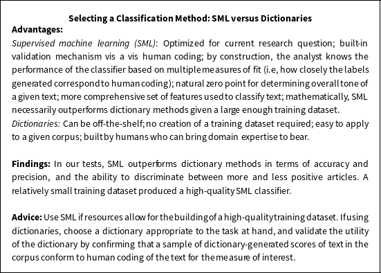
4 Selecting a Classification Method: Supervised Machine Learning versus Dictionaries
Dictionary methods and SML methods constitute the two primary approaches for coding the tone of large amounts of text. Here, we describe each method, discuss the advantages and disadvantages of each, and assess the ability of a number of dictionaries and SML classifiers (1) to correctly classify documents labeled by humans and (2) to distinguish between more and less positive documents.Footnote 40
A dictionary is a user-identified set of features or terms relevant to the coding task where each feature is assigned a weight that reflects the feature’s user-specified contribution to the measure to be produced, usually +1 for positive and -1 for negative features. The analyst then applies some decision rule, such as summing over all the weighted feature values, to create a score for the document. By construction, dictionaries code documents on an ordinal scale, that is, they sort documents as to which are more or less positive or negative relative to one other. If an analyst wants to know which articles are positive or negative, they need to identify a cut point (zero point). We may assume an article with more positive terms than negative terms is positive, but we do not know ex ante if human readers would agree. If one is interested in relative tone, for example, if one wanted to compare the tone of documents over time, the uncertainty about the cut point is not an issue.
The analyst selecting SML follows three broad steps. First, a sample of the corpus (the training dataset) is coded (classified) by humans for tone, or whatever attribute is being measured (the text is labeled). Then a classification method (machine learning algorithm) is selected and the classifier is trained to predict the label assigned by the coders within the training dataset.Footnote 41 In this way the classifier “learns” the relevant features of the dataset and how these features are related to the labels. Multiple classification methods are generally applied and tested for minimum levels of accuracy using cross-validation to determine the best classifier. Finally, the chosen classifier is applied to the entire corpus to predict the sentiment of all unclassified articles (those not labeled by humans).
Dictionary and SML methods allow analysts to code vast amounts of text that would not be possible with human coding, and each presents unique advantages but also challenges. One advantage of dictionaries is that many have already been created for a variety of tasks, including measuring the tone of text. If an established dictionary is a good fit for the task at hand, then it is relatively straightforward to apply it. However, if an appropriate dictionary does not already exist, the analyst must create one. Because creating a dictionary requires identifying features and assigning weights to them, it is a difficult and time-consuming task. Fortunately, humans have been “trained” on a lifetime of interactions with language and thus can bring a tremendous amount of prior information to the table to assign weights to features. Of course, this prior information meets many practical limitations. Most dictionaries will code unigrams, since if the dictionary is expanded to include bigrams or trigrams the number of potential features increases quickly and adequate feature selection becomes untenable. And all dictionaries necessarily consider a limited and subjective set of features, meaning not all features in the corpus and relevant to the analysis will be in the dictionary. It is important, then, that analysts carefully vet their selection of terms. For example, Muddiman and Stroud (Reference Muddiman and Stroud2017) construct dictionaries by asking human coders to identify words for inclusion, and then calculate the inter-coder reliability of coder suggestions. Further, in assigning weights to each feature, analysts must make the assumption that they know the importance of each feature in the dictionary and that all text not included in the dictionary has no bearing on the tone of the text.Footnote 42 Thus, even with rigorous validation, dictionaries necessarily limit the amount of information that can be learned from the text.
In contrast, when using SML the relevant features of the text and their weights are estimated from the data.Footnote 43 The feature space is thus likely to be both larger and more comprehensive than that used in a dictionary. Further, SML can more readily accommodate the use of n-grams or co-occurrences as features and thus partially incorporate the context in which words appear. Finally, since SML methods are trained on data where humans have labeled an article as “positive” or “negative”, they estimate a true zero point and can classify individual documents as positive or negative. The end result is that much more information drives the subsequent classification of text.
But SML presents its own challenges. Most notably it requires the production of a large training dataset coded by humans and built from a random set of texts in which the features in the population of texts are well represented. Creating the training dataset itself requires the analyst to decide a unit of analysis to code, the number of coders to use per object, and the number of objects to be coded. These decisions, as we show above, can affect the measure of tone produced. In addition, it is not clear how generalizable any training dataset is. For example, it may not be true that a classifier trained on data from the New York Times is optimal for classifying text from USA Today or that a classifier trained on data from one decade will optimally classify articles from a different decade.
Dictionary methods allow the analyst to bypass these tasks and their accompanying challenges entirely. Yet, the production of a human-coded training dataset for use with SML allows the analyst to evaluate the performance of the classifier with measures of accuracy and precision using cross-validation. Analysts using dictionaries typically have no (readily available) human-coded documents with which to evaluate classifier performance. Even when using dictionaries tested by their designers, there is no guarantee that the test of the dictionary on one corpus for one task or within one domain (e.g., newspaper articles) validates the dictionary’s use on a different corpus for a different task or domain (e.g., tweets). In fact the evaluation of the accuracy of dictionaries is difficult precisely because of the issue discussed earlier, that they have no natural cut point to distinguish between positive and negative documents. The only way to evaluate performance of a dictionary is to have humans code a sample of the corpus and examine whether the dictionary assigns higher scores to positive documents and lower scores to negative documents as evaluated by humans. For example, Young and Soroka (Reference Young and Soroka2012) evaluate Lexicoder by binning documents based on scores assigned by human coders and reporting the average Lexicoder score for documents in each bin. By showing that the Lexicoder score for each bin is correlated with the human score, they validate the performance of Lexicoder.Footnote 44 Analysts using dictionaries “off-the-shelf” could perform a similar exercise for their applications, but at that point the benefits of using a dictionary begin to deteriorate. In any case, analysts using dictionaries should take care both in validating the inclusion of terms to begin with and validating that text containing those terms has the intended sentiment.
Given the advantages and disadvantages of the two methods, how should the analyst think about which is likely to perform better? Before moving to empirics, we can perform a thought experiment. If we assume both the dictionary and the training dataset are of high quality, then we already know that if we consider SML classifiers that utilize only words as features, it is mathematically impossible for dictionaries to do as well as an SML model trained on a large enough dataset if we are testing for accuracy within sample. The dictionary comes with a hard-wired set of parameter values for the importance of a predetermined set of features. The SML model will estimate parameter values optimized to minimize error of the classifier on the training dataset. Thus, SML will necessarily outperform the dictionary on that sample. So the relevant question is, which does better out of sample? Here, too, since the SML model is trained on a sample of the data, it is guaranteed to do better than a dictionary as long as it is trained on a large enough random sample. As the sample converges to the population—or as the training dataset contains an ever increasing proportion of words encountered—SML has to do better than a dictionary, as the estimated parameter values will converge to the true parameter values.
While a dictionary cannot compete with a classifier trained on a representative and large enough training dataset, in any given task dictionaries may outperform SML if these conditions are not met. Dictionaries bring rich prior information to the classification task: humans may produce a topic-specific dictionary that would require a large training dataset to outperform it. Similarly, a poor training dataset may not contain enough (or good enough) information to outperform a given dictionary. Below we compare the performance of a number of dictionaries with SML classifiers in the context of coding sentiment about the economy in the New York Times, and we examine the role of the size of the training dataset set in this comparison in order to assess the utility of both methods.
4.1 Comparing Classification Methods
The first step in comparing the two approaches is to identify the dictionaries and SML classifiers we wish to compare. We consider three widely used sentiment dictionaries. First, SentiStrength is a general sentiment dictionary optimized for short texts (Thelwall et al. Reference Thelwall, Buckley, Paltoglou, Cai and Kappas2010). It produces a positive and negative score for each document based on the word score associated with the strongest positive word (between 0 and 4) and the strongest negative word (between 0 and -4) in the document that are also contained in the dictionary. The authors did not choose to generate a net tone score for each document. We do so by summing these two positive and negative sentiment scores, such that document scores range from -4 to +4. Second, Lexicoder is a sentiment dictionary designed specifically for political text (Young and Soroka Reference Young and Soroka2012). It assigns every n-gram in a given text a binary indicator if that n-gram is in its dictionary, coding for whether it is positive or negative. Sentiment scores for documents are then calculated as the number of positive minus the number of negative terms divided by the total number of terms in the document. Third, Hopkins et al. (Reference Hopkins, Kim and Kim2017) created a relatively simple dictionary proposed of just twenty-one economic terms.Footnote 45 They calculate the fraction of articles per month mentioning each of the terms. The fractions are summed, with positive and negative words having opposite signs, to calculate net tone in a given time interval. We extend their logic to predict article-level scores by summing the number of unique positive stems and subtracting the number of unique negative stems in an article to produce a measure of sentiment.
We train an SML classifier using a dataset generated from 4,400 unique articles (Dataset 5AC in Appendix Table 1) in the New York Times randomly sampled from the years 1947 to 2014. Between three and ten CrowdFlower workers coded each article for relevance. At least one coded 4,070 articles as relevant with an average of 2.51 coders coding each relevant article for tone using the 9-point scale. The optimal classifier was selected from a set of single-level classifiers including logistic regression (with L2 penalty), Lasso, ElasticNet, SVM, Random Forest, and AdaBoost.Footnote 46 Based on accuracy and precision evaluated using UG Truth and CF Truth, we selected regularized logistic regression with L2 penalty with up to 75,000 n-grams appearing in at least three documents and no more than 80% of all documents, including stopwords, and stemming.Footnote 47 Appendix Table 12 presents the n-grams most predictive of positive and negative tone.

Figure 3. Performance of SML and Dictionary Classifiers—Accuracy and Precision. Note: Accuracy (percent correctly classified) and precision (percent of positive predictions that are correct) for the ground truth dataset coded by ten CrowdFlower coders. The dashed vertical lines indicate the baseline level of accuracy or precision (on any category) if the modal category is always predicted. The corpus used in the analysis is based on the keyword search of The New York Times 1980–2011 (see the text for details).

Figure 4. Accuracy of the SML Classifier as a Function of Size of the Training Dataset. Note: We drew ten random samples of 250 articles each from the full training dataset (Dataset 5AC, Appendix Table 1) of 8,750 unique codings of 4,400 unique articles (three to five crowd coders labeled each article) in the New York Times randomly sampled from the years 1947 to 2014. Using the same method as discussed in the text, we estimated the parameters of the SML classifier on each of these ten samples. We then used each of these estimates of the classifier to predict the tone of articles in CF Truth. We repeated this process for sample sizes of 250 to 8,750 by increments of 250, recording the percent of articles correctly classified.
We can now compare the performance of each approach. We begin by assessing them against the CF Truth dataset, comparing the percent of articles for which each approach (1) correctly predicts the direction of tone coded at the article-segment level by humans (accuracy) and (2) specifically for articles predicted to be positive, those predictions align with human annotations (precision).Footnote
48
 $^{,}$
Footnote
49
Then for SML, we consider the role of training dataset size and the threshold selected for classification. Then we assess accuracy for the baseline SML classifier and Lexicoder for articles humans have coded as particularly negative or positive and those about which our coders are more ambivalent.Footnote
50
$^{,}$
Footnote
49
Then for SML, we consider the role of training dataset size and the threshold selected for classification. Then we assess accuracy for the baseline SML classifier and Lexicoder for articles humans have coded as particularly negative or positive and those about which our coders are more ambivalent.Footnote
50
4.1.1 Accuracy and Precision
Figure 3 presents the accuracy (left panel) and relative precision (right panel) of the dictionary and SML approaches. We include a dotted line in each panel of the figure to represent the percent of articles in the modal category. Any classifier can achieve this level of accuracy simply by always assigning each document to the modal category. Figure 3 shows that only SML outperform the naive guess of the modal category. The baseline SML classifier correctly predicts coding by crowd workers in 71.0% of the articles they coded. In comparison, SentiStrength correctly predicts 60.5%, Lexicoder 58.6%, and the Hopkins 21-Word Method 56.9% of the articles in CF Truth. The relative performance of the SML classifier is even more pronounced with respect to precision, which is the more difficult task here as positive articles are the rare category. Positive predictions from our baseline SML model are correct 71.3% of the time while for SentiStrength this is true 37.5% of the time and Lexicoder and Hopkins 21-Word Method do so 45.7% and 38.5% of the time, respectively. In sum, each of the dictionaries is both less accurate and less precise than the baseline SML model.Footnote 51
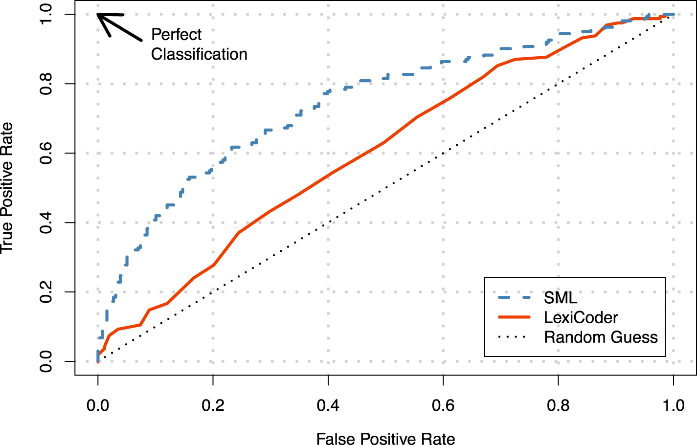
Figure 5. Receiver Operator Characteristic Curve: Lexicoder versus SML. Note: The x-axis gives the false positive rate—the proportion of all negatively toned articles in CF Truth that were classified as positively toned—and the y-axis gives the true positive rate—the proportion of all positively toned articles in CF Truth that were classified as positive. Each point on the curve represents the misclassification rate for a given classification threshold. The corpus used in the analysis is based on the keyword search of The New York Times 1980–2011.
What is the role the training dataset size in explaining the better accuracy and precision rates of the SML classifier? To answer this question, we drew ten random samples of 250 articles each from the full CF Truth training dataset. Using the same method as above, we estimated the parameters of the SML classifier on each of these ten samples. We then used each of these estimates of the classifier to predict the tone of articles in CF Truth, recording accuracy, precision, and recall for each replication.Footnote 52 We repeated this process for sample sizes of 250 to 8,750 by increments of 250. Figure 4 presents the accuracy results, with shaded areas indicating the 95% confidence interval. The x-axis gives the size of the training dataset and the y-axis reports the average accuracy in CF Truth for the given sample size. The final point represents the full training dataset, and as such there is only one accuracy rate (and thus no confidence interval).
What do we learn from this exercise? Using the smallest training dataset (250), the accuracy of the SML classifier equals the percent of articles in the modal category (about 63%). Further, accuracy improves quickly as the size of the training dataset increases. With 2,000 observations, SML is quite accurate, and there appears to be very little return for a training dataset with more than 3,000 articles. While it is clear that in this case 250 articles is not a large enough training dataset to develop an accurate SML classifier, even using this small training dataset the SML classifier has greater accuracy with respect to CF Truth than that obtained by any of the dictionaries.Footnote 53

Figure 6. Classification Accuracy in CF Truth as a Function of Article Score (Lexicoder) and Predicted Probability an Article is Positive (SML Classification). Note: Dictionary scores and SML predicted probabilities are assigned to each article in the CF Truth dataset. Articles are then assigned to a decile based on this score. Each block or circle on the graph represents accuracy within each decile, which is determined based on coding from CF Truth. The corpus used in the analysis is based on the keyword search of The New York Times 1980–2011.
An alternative way to compare SML to dictionary classifiers is to use a receiver operator characteristic, or ROC, curve. An ROC curve shows the ability of each classifier to correctly predict whether the tone of an article is positive in CF Truth for any given classification threshold. In other words, it provides a visual description of a classifier’s ability to separate negative from positive articles across all possible classification rules. Figure 5 presents the ROC curve for the baseline SML classifier and the Lexicoder dictionary.Footnote
54
The x-axis gives the false positive rate—the proportion of all negatively toned articles in CF Truth that were classified as positively toned—and the y-axis gives the true positive rate—the proportion of all positively toned articles in CF Truth that were classified as positive. Each point on the curve represents the misclassification rate for a given classification threshold. Two things are of note. First, for almost any classification threshold, the SML classifier gives a higher true positive rate than Lexicoder. Only in the very extreme cases in which articles are classified as positive only if the predicted probability generated by the classifier is very close to 1.0 (top right corner of the figure) does Lexicoder misclassify articles slightly less often. Second, the larger the area under the ROC curve (AUC), the better the classifier’s performance. In this case the AUC of the SML classifier (0.744) is significantly greater (
 $p=0.00$
) than for Lexicoder (0.602). This finding confirms that the SML classifier has a greater ability to distinguish between more positive versus less positive articles.
$p=0.00$
) than for Lexicoder (0.602). This finding confirms that the SML classifier has a greater ability to distinguish between more positive versus less positive articles.
4.1.2 Ability to Discriminate
One potential shortcoming of focusing on predictive accuracy may be that, even if SML is better at separating negative from positive articles, perhaps dictionaries are better at capturing the gradient of potential values of sentiment, from very negative to very positive. If this were the case, then dictionaries could do well when comparing the change in sentiment across articles or between groups of articles. In fact, this is what we are often trying to do when we examine changes in tone from month to month.
To examine how well each method gauges relative tone, we conduct an additional validation exercise similar to that performed by Young and Soroka (Reference Young and Soroka2012) to assess the performance of Lexicoder relative to the SML classifier. Instead of reporting accuracy at the article level, we split our CF Truth sample into sets of deciles according to (1) the sentiment score assigned by Lexicoder and (2) the predicted probability according to the SML classifier. We then measure the proportion of articles that crowd workers classified as positive within each decile. In other words, we look at the 10% of articles with the lowest sentiment score according to each method and count how many articles in CF Truth are positive within this bucket; we then repeat this step for all other deciles.
As Figure 6 shows, while in general articles in each successive bin according to the dictionary scores were more likely to have been labeled as positive in CF Truth, the differences are not as striking as with the binning according to SML. The groups of articles the dictionary places in the top five bins are largely indistinguishable in terms of the percent of articles labeled positive in CF Truth and only half of the articles with the highest dictionary scores were coded positive in CF Truth. The SML classifier shows a clearer ability to distinguish the tone of articles for most of the range, and over 75% of articles classified with a predicted probability of being positive in the top decile were labeled as such in CF Truth. In short, even when it comes to the relative ranking of articles, the dictionary does not perform as well as SML and it is unable to accurately distinguish less positive from more positive articles over much of the range of dictionary scores.
4.2 Selecting a Classification Method: Conclusions from the Evidence
Across the range of metrics considered here, SML almost always outperformed the dictionaries. In analyses based on a full training dataset—produced with either CrowdFlower workers or undergraduates—SML was more accurate and had greater precision than any of the dictionaries. Moreover, when testing smaller samples of the CF training dataset, the SML classifier was more accurate and had greater precision even when trained on only 250 articles. Further, our binning analysis with Lexicoder showed that Lexicoder was not as clearly able to distinguish the relative tone of articles in CF Truth as was SML; and the ROC curve showed that the accuracy of SML outperformed that of Lexicoder regardless of the threshold used for classification. Our advice to analysts is to use SML techniques to develop measures of tone rather than to rely on dictionaries.
5 Recommendations for Analysts of Text
The opportunities afforded by vast electronic text archives and machine classification of text for the measurement of a number of concepts, including tone, are in a real sense unlimited. Yet in a rush to take advantage of the opportunities, it is easy to overlook some important questions and to underappreciate the consequences of some decisions.
Here, we have discussed just a few of the decisions that face analysts in this realm. Our most striking, and perhaps surprising, finding is that something as simple as how we choose the corpus of text to analyze can have huge consequences for the measure we produce. Perhaps more importantly, we found that analyses based on the two distinct sets of documents produced very different measures of the quantity of interest: sentiment about the economy. For the sake of transparency and portability, we recommend the analyst use keyword searches, rather than proprietary subject classifications. When deciding on the unit to be coded, we found that coding article segments was more efficient for our task than coding sentences. Further, segment-level coding has the advantage that the human coders are working closer to the level of object that is to be classified (here, the article), and it has the nontrivial advantage that it is cheaper and more easily implemented in practice. Thus, while it is possible that coding at the sentence level would produce a more precise classifier in other applications, our results suggest that coding at the segment level seems to be the best default. We also find that the best course of action in terms of classifier accuracy is to maximize the number of unique objects coded, irrespective of the selected coder pool or the application of interest. Doing so produces more efficient estimates than having additional coders code an object. Finally, based on multiple tests, we recommend using SML for sentiment analysis rather than dictionaries. Using SML does require the production of a training dataset, which is a nontrivial effort. But the math is clear: given a large enough training dataset, SML has to outperform a dictionary. And, in our case at least, the size of the training dataset required was not very large.
From these specific recommendations, we can distill overarching pieces of advice: (1) use transparent and reproducible methods in selecting a corpus and (2) classify by machine, but verify by human means. But our evidence suggests two lessons more broadly. First, for analysts using text as data, there are decisions at every turn, and even the ones we assume are benign may have meaningful downstream consequences. Second, every research question and every text-as-data enterprise is unique. Analysts should do their own testing to determine how the decisions they are making affect the substance of their conclusions, and be mindful and transparent at all stages in the process.
Acknowledgments
We thank Ken Benoit, Bryce Dietrich, Justin Grimmer, Jennifer Pan, and Arthur Spirling for their helpful comments and suggestions to a previous version of the paper. We thank Christopher Schwarz for writing code for simulations for the section on more documents versus more coders (Figure 2). We are indebted to Stuart Soroka and Christopher Wlezien for generously sharing data used in their past work, and for constructive comments on previous versions of this paper.
Funding
This material is based in part on work supported by the National Science Foundation under IGERT Grant DGE-1144860, Big Data Social Science, and funding provided by the Moore and Sloan Foundations. Nagler’s work was supported in part by a grant from the INSPIRE program of the National Science Foundation (Award SES-1248077).
Data Availability Statement
Replication code for this article has also been published in Code Ocean, a computational reproducibility platform that enables users to run the code, and can be viewed interactively at doi:10.24433/CO.4630956.v1. A preservation copy of the same code and data can also be accessed via Dataverse at doi:10.7910/DVN/MXKRDE.
Supplementary material
For supplementary material accompanying this paper, please visit https://doi.org/10.1017/pan.2020.8.


