

Introduction
One of the major characteristics of the Arctic climate system is the presence of sea-ice (McPhee, Reference McPhee2008; Wadhams, Reference Wadhams2000). The sea-ice cover in the Arctic Ocean is constantly in motion and highly dynamic in both space and time. It is forced by thermodynamic and dynamic processes that result in seasonal and inter-annual variations in ice thickness, extent, and areal concentration. Sea-ice drift is an important indicator of these processes, and is also important in terms of the transport of freshwater and latent heat. The Beaufort Gyre (BG) and the transpolar drift (TPD) characterise the two primary circulation patterns of sea-ice drift in the Arctic Ocean. The BG is a large-scale ocean circulation pattern in the Amerasian Basin. It is a unique anticyclonic circulation regime within the Arctic Ocean physical environment driven by a set of specific atmospheric, sea-ice, and oceanic conditions that are interrelated with pan-Arctic as well as global climate systems (Dukhovskoy, Johnson, & Proshutinsky, Reference Dukhovskoy, Johnson and Proshutinsky2004; Krishfield et al., Reference Krishfield, Proshutinsky, Tateyama, Williams, Carmack, McLaughlin and Timmermans2014; Morison et al., Reference Morison, Kwok, Peralta-Ferriz, Alkire, Rigor, Andersen and Steele2012; Proshutinsky et al., Reference Proshutinsky, Krishfield, Timmermans, Toole, Carmack, McLaughlin and Shimada2009; Proshutinsky, Bourke, & McLaughlin, Reference Proshutinsky, Bourke and McLaughlin2002). Sea-ice drift within the BG is predominantly characterised by anticyclonic circulation, with relatively brief periods of reversal in direction occurring intermittently throughout the annual cycle (Ledrew, Johnson, & Maslanik, Reference Ledrew, Johnson and Maslanik2007; Lukovich & Barber, Reference Lukovich and Barber2006; Preller & Posey, Reference Preller and Posey1989). The TPD starts along the Siberian coast and ends with ice exiting through Fram Strait after crossing the region of the geographical North Pole. A study conducted by Zhao and Liu (Reference Zhao and Liu2007) for the winters (December to March) 1988 to 2003 divided the sea-ice drift patterns into four categories on the basis of weak, strong and normal BG with a combination of weak/strong cyclonic motion in the Eurasian Basin. Wang and Zhao (Reference Wang and Zhao2012) also defined four primary drift pattern types on the basis of mean ice velocity fields and sea level pressure (BG + TPD, anticyclonic drift, cyclonic drift and double gyre drift) that account for 81% of the total ice drift patterns over the period of 1979–2006. The motion of ice in Fram Strait is parallel to the east coast of Greenland, with the drift speeds decreasing westwards until stationary landfast sea-ice is encountered during the winter period.
The main features of the large-scale sea-ice drift pattern in the Arctic Ocean have been well established for decades (Colony & Thorndike, Reference Colony and Thorndike1984; Gordienko, Reference Gordienko and Thurston1958; Olason & Notz, Reference Olason and Notz2014); however, the system displays substantial variability in both space and time (Martin & Gerdes, Reference Martin and Gerdes2007; Proshutinsky & Johnson, Reference Proshutinsky and Johnson1997) and is affected by large-scale atmospheric pressure patterns that are currently experiencing change due to sea-ice concentration changes in winter (Barber et al., Reference Barber, Hop, Mundy, Else, Dmitrenko, Tremblay and Rysgaard2015) and changes in hemispheric pressure patterns (Overland & Wang, Reference Overland and Wang2005) and the extensive loss of the oldest sea-ice types. The increasing coverage of the younger sea-ice types within the Arctic Ocean (Maslanik et al., Reference Maslanik, Fowler, Stroeve, Drobot, Zwally, Yi and Emery2007; Maslanik, Stroeve, Fowler, & Emery, Reference Maslanik, Stroeve, Fowler and Emery2011) and concurrent reduction of the multiyear ice cover (Kwok, Reference Kwok2007) are probably the factors that affect the drift speeds and their patterns. Recently, an increase in sea-ice drift speeds has been observed over the central Arctic and the regions of TPD (Häkkinen, Proshutinsky, & Ashik, Reference Häkkinen, Proshutinsky and Ashik2008; Rampal, Weiss, & Marsan, Reference Rampal, Weiss and Marsan2009; Spreen, Kwok, & Menemenlis, Reference Spreen, Kwok and Menemenlis2011). Häkkinen et al. (Reference Häkkinen, Proshutinsky and Ashik2008) found a positive trend in the TPD speed for 1950–2006 using observations from the Russian North Pole stations, various expedition camps, and the International Arctic Buoy Program (IABP) data. A stronger TPD has been shown to lead to the shorter residence time of sea-ice in the Arctic Ocean and to promote increased ice export through Fram Strait (Haller, Brümmer, & Müller, Reference Haller, Brümmer and Müller2014). Kwok, Spreen and Pang (Reference Kwok, Spreen and Pang2013) showed that over 90% of the Arctic Ocean experienced positive trends in drift speed from 1982 to 2010, correlating with the regions that experienced reductions in multiyear sea-ice coverage. Attention was brought to the changed TPD speed during the drift of the French vessel Tara in 2006–2007 when it took half the time to drift about the same distance as the Norwegian vessel Fram did in 1893–1896 (Gascard et al., Reference Gascard, Festy, le Goff, Weber, Bruemmer, Offermann and Bottenheim2008). Sea-ice drift speeds and patterns act as catalysts in the export of sea-ice and play a fundamental role in the ongoing reductions in the Arctic sea-ice extent and volume. However, the temporal (annual and inter-annual) and spatial variability in the BG and TPD remain poorly understood and described over recent timescales; in particular, with regards to the determination of any trends that may be emerging as a consequence of the rapid change in the concentration, thickness and type of sea-ice in the Arctic Ocean (Barber et al., Reference Barber, Galley, Asplin, De Abreu, Warner, Pućko and Julien2009).
In this paper, we examine the winter season large-scale multi-decadal ice drift trends to help identify a baseline on how the ice drift in the Arctic Ocean varies over both space and time. The primary objective of this study is to analyse passive-microwave derived sea-ice drift over the past 36 winters (1979–2015) to identify changes and variability in the Arctic Ocean ice drift patterns over time. More specifically, we address the following research questions: (1) Can winter sea-ice drift data be used to unambiguously characterise large-scale features of Northern Hemisphere ice motion? (2) Do these patterns extend beyond the expected BG and TPD? (3) What are the basin-wide spatial trends in these sea-ice drift patterns for the 36 winters (Oct–Apr) during 1979–2015? (4) What are the basin-wide temporal trends in these ice motion fields?
Methods
Data description
Passive-microwave derived sea-ice drift products are provided by different institutions and have been widely used in sea-ice studies and for sea-ice drift speed analyses (e.g. Kwok & Rothrock, Reference Kwok and Rothrock2009; Kwok et al., Reference Kwok, Spreen and Pang2013; Spreen et al., Reference Spreen, Kwok and Menemenlis2011). Mean monthly gridded sea-ice motion vectors were obtained from the National Snow and Ice Data Center (NSIDC) and Polar Pathfinder Sea Ice Mean Monthly Motion Vectors (Version 3) data were chosen because of their homogeneous spatial coverage and long-term availability. The product provided by NSIDC contained the monthly gridded fields of sea-ice motion on a 25 km Equal-Area Scalable Earth (EASE) grid for the period 1979 to 2015 (Tschudi, Fowler, Maslanik, Stewart, & Meier, Reference Tschudi, Fowler, Maslanik, Stewart and Meier2016). The sea-ice motion vectors are available in 361 × 361 pixel EASE grid projection. NSIDC obtains the motion vectors after processing data from a variety of satellite-based sensors, such as AMSR-E, AVHRR, SMMR, SSM/I, SSMIS, wind vectors from NCEP/NCAR Reanalysis, and buoy observations from the International Arctic Buoy Program (IABP). The daily gridded ice motion vectors obtained by NSIDC are computed from an algorithm that performs optimal interpolation, using several data sources. Further, the monthly gridded ice motion vectors distributed by NSIDC are obtained by averaging the daily ice motion vectors. For monthly means, NSIDC uses data from a minimum of 20 days; otherwise, the corresponding site is marked as missing data. Features in the ice that were visible in satellite images are tracked by an automated spatial correlation method and the drift velocity is subsequently calculated from the displacement of the observed features. A description of the dataset and the sea-ice motion retrieval algorithm can be found in Tschudi et al. (Reference Tschudi, Fowler, Maslanik, Stewart and Meier2016). Previous studies have demonstrated the uncertainty estimates for NSIDC and the persistent artifacts that can be observed in the NSIDC sea-ice motion dataset (Sumata et al., Reference Sumata, Lavergne, Girard-Ardhuin, Kimura, Tschudi, Kauker and Gerdes2014; Szanyi, Lukovich, Barber, & Haller, Reference Szanyi, Lukovich, Barber and Haller2016). Schwegmann, Haas, Fowler, & Gerdes (Reference Schwegmann, Haas, Fowler and Gerdes2011) found the absolute differences (buoy-satellite) are 0.062 ± 0.067 ms−1 for the zonal and 0.065 ± 0.064 ms−1 for the meridional drift. However, no such bias has been observed for long-term time-averaged data as used here. Only winter data have been used in this study because effects of weather, atmospheric moisture, and surface melt during the summer can have a detrimental effect on the data quality and the analysis (Sumata, Kwok, Gerdes, Kauker, & Karcher, Reference Sumata, Kwok, Gerdes, Kauker and Karcher2015).
Sea-ice drift speed and pattern analysis
As the original drift vector components, u and v, represent the drift vectors in horizontal and vertical components, respectively, the vectors were rotated along the longitudes to obtain their zonal (east–west) and meridional (north–south) drift components. The equations used in the rotation of the vectors are as follows:
 $$U = u.^{\rm{_*}}\rm cos \left({{{\oslash}}} \right) + v.^{\rm{_*}}sin \left( {\rm{{\oslash}}} \right)$$
 $$V = - u.^{\rm{_*}}sin \left( {\rm{{\oslash}}} \right) + v.^{\rm{_*}}cos\left( {\rm{{\oslash}}} \right)$$
where ø denotes the longitude, and U and V represent the zonal and meridional components of the ice drift. It should be noted that the ice drift was evaluated for October–April from 1979 to 2015, resulting in 252 months of gridded data. Sea-ice drift speed (magnitude of ice drift) was computed using the zonal and meridional components of ice drift, i.e. s = (U2 + V2)1/2 and drift anomalies for 36 years individually were calculated with respect to the average (1979–2015) winter season drift.
The boundaries between the main circulation patterns were identified based on the 36-year winter average sea-ice motion (Fig. 1a). This was done by tracking the ice motion vectors at three-day intervals and using the nearest pixel to that location to continue the same process to demarcate the exchange boundary between the BG and TPD, TPD and the Kara Sea. Thus, the boundary is defined here as a transect across which mean ice transport is zero, i.e. as an average over 36 winters there was no net exchange of ice (in terms of surface area) across this transect (Fig. 1b).

Fig. 1. (a) Mean Arctic sea-ice drift patterns of the 36 winter seasons overlaid over the mean winter sea ice drift speed (cm/s) from October 1979 to April 2015. (b) Ice drift values for across and along exchange boundary transect.
Statistical analysis of sea-ice drift patterns
Empirical Orthogonal Function (EOF) analysis is one of the more widely used multivariate statistical techniques used to investigate spatial modes (i.e. patterns) of variability and how they change with time (Nigam & Baxter, Reference Nigam, Baxter, North, Pyle and Zhang2015). We applied the EOF analysis, also known as Principal Component Analysis (PCA), to investigate the spatial variability in the dataset. In this study, we employed the EOF technique to analyse the mean winter sea-ice drift patterns over 36 winter seasons from 1979 to 2015. EOF gives Eigen modes of variability and corresponding principal component time series for spatiotemporal data analysis. For the purpose of analysing the vector dataset the 3-dimensional matrix was converted to a 2-dimensional matrix. In the 3-D matrix, the first two dimensions were spatial and the third dimension was temporal, equally spaced in time. In the conversion, zonal (u) and meridional (v) components of the ice drift speed were arranged underneath each other to form a single matrix in which the rows 1 to 361 indicate the u component and rows 362 to 722 indicate the v component. The columns in the matrix represent the spatial scale of the dataset. Output EOF maps have the same dimensions as the input matrix. Furthermore, the resulting vectors have been multiplied by –1 to obtain the vectors in the correct directions.
Regression analysis was used to obtain the trends in the sea-ice drift speed anomalies over the 36-year winter period. Previous studies have used the scalar amplitude of the ice drift vectors to analyse the trend in the sea-ice drift speeds (Kwok et al., Reference Kwok, Spreen and Pang2013). However, trends in anomalies are analysed in this study to cope with the uncertainties in the result that might appear in the case of absolute values. Linear trends at each grid point were separated for the zonal and meridional components of the ice drift to examine changes in the relative contributions of each over the last several decades.
Results and discussion
Classification and description of Arctic sea-ice drift patterns
Figure 1a shows the mean Arctic sea-ice motion of the 36 winter seasons (1979–2015) obtained by averaging 252 months of gridded sea-ice vector data for the period October 1979 to April 2015. This mean Arctic sea-ice motion map shows two distinct features: an anticyclonic motion in the Canadian basin, i.e. BG, and TPD that drives the ice from the Laptev Sea across the pole to the Fram Strait. In addition to these two dominant Arctic circulation patterns there exists a motion system in the Eurasian Basin moving ice from the Kara Sea (KS) via the ocean route between Franz Josef Land and Novaya Zemlya. The average drift speeds from 1979 to 2015 were highest in the Fram Strait, with drift speeds as high as 10.5 cm/s (9 km/day). The range of drift speeds in BG, TPD and KS is 4–6 cm/s, 3–4 cm/s and 3–4 cm/s, respectively. High drift speeds are also observed in Baffin Bay (up to 6 cm/s); however, only circulation patterns within the Arctic Basin and the flow through the Fram Strait are discussed in this paper.
The clear demarcation of these features indicates that the mean monthly winter dataset can be used to study these large-scale circulation regimes and their variability over time. The mean circulation pattern is in keeping with earlier studies (i.e. Gordienko, Reference Gordienko and Thurston1958; Martin & Gerdes, Reference Martin and Gerdes2007; Proshutinsky & Johnson, Reference Proshutinsky and Johnson1997; Thorndike & Colony, Reference Thorndike and Colony1982), while also illustrating a third ice drift feature in the Kara Sea.
The transects in Fig. 1a demarcate the boundaries across which the component normal to the boundary of the sea-ice drift is zero (Fig. 1b) for the mean 1979–2015 sea-ice drift, i.e. on average over 36 years no ice-flux occurs across this boundary. The average motion over winter shows that the sea-ice to the left of transect line 1 will circulate within the BG and remain within the Arctic Ocean, while sea-ice to the right has a drift trajectory that will eventually exit the Arctic Ocean. Ice drift across the transect is calculated for each winter’s average ice drift between 1979 and 2015 (Fig. 2). Negative values correspond to winters when the flow of ice from BG towards TPD exceeds the flow towards the BG across transect 1. Such situations occur when there is the dominance of the BG over the Arctic Basin when the centre of the gyre shifts to close proximity to the North Pole. Increasing variability in the mean drift perpendicular to transect 1 is observed, with variance of 0.14 during 1979–1996 and 0.26 during 1997–2015.

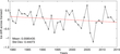
Fig. 2. Average winter sea-ice motion across transect 1 (Fig. 1a) separating the 36-winter (1979-2015) average Beaufort Gyre and Transpolar Drift patterns.
In general, the positive values in Fig. 2 relate to winters with a weaker BG, whereas negative values relate to winters when the BG crosses transect 1. Drift patterns for each winter between 1979 and 2015 are shown in Supplementary Fig. S1.
During winter 1979, the basic features of the climatology (Fig. 1a) were evident, but the BG covered a larger area while the TPD observed the shift towards the eastern side of the Arctic Ocean and the ice drift from the KS contributed to the TPD. Until 1986, the drift speeds observed in the Fram Strait were very low, with the maximum speed of 10 cm/s observed in the winter of 1982. Very high drift speeds were observed in the Fram Strait in the winter of 1987, with drift speeds approaching 14 cm/s (Fig. S1). The rest of the Arctic Basin experienced drift speeds of less than 3 cm/s until 1997, when very high drift speeds, ranging between 5 and 10 cm/s, were observed for the first time in the region north of Alaska. However, drift speeds in the Fram Strait were not as high as in previous years. The ice drift speeds in the Fram Strait ranged between 8 and 12 cm/s in 1997. High drift speeds (5–10 cm/s) were observed in the region north of the Alaskan coast until 2005, when the BG was completely missing from the Arctic Basin (Fig. S1). Rigor, Wallace, & Colony (Reference Rigor, Wallace and Colony2002) have linked the variability in BG ice circulation to variability in the Beaufort High, described in terms of Arctic Oscillation (AO). The negative phase of the AO is associated with a strong BG. Low drift speeds were observed in the Arctic in 2006, with values in the range of 0–6 cm/s. That year the flow through the Fram Strait was mostly from the Kara Sea, with the drift speeds ranging between 10 and 13 cm/s. In 2006, mean winter drift speeds as high as 13 cm/s were also observed in the Barents Sea.
In 2007, the BG contributed significantly to the TPD and, for the first time, mean winter drift speeds as high as 10–13 cm/s were observed in the western part of the gyre (Fig. S1). It corresponds to the lowest value on record for drift across transect 1 (Fig. 2). Petty, Hutchings, Richter-Menge, & Tschudi (Reference Petty, Hutchings, Richter-Menge and Tschudi2016) also found amplified anticyclonic drift in the 2000s compared to the 1980s/1990s. The mean winter drift speeds observed in the Fram Strait were also high, ranging between 13 and 15 cm/s. The majority of ice transport in Beaufort Sea occurs from October to May, which provides replenishment for ice lost during the summer months (Howell, Brady, Derksen, & Kelly, Reference Howell, Brady, Derksen and Kelly2016). However, Stroeve et al. (Reference Stroeve, Maslanik, Serreze, Rigor, Meier and Fowler2011) found that the AO turned strongly negative during the winter of 2009 and, despite the substantial transport of thick ice into the Beaufort and Chukchi seas, the majority of the ice did not survive the summer. In 2011 a reversal was observed, moving the ice diagonally across the Arctic Basin from the Laptev Sea towards the Canadian Archipelago and onwards to the north of Alaska (Fig. S1). This drift of ice towards the Bering Strait has also been observed by Babb, Galley, Asplin, Lukovich, & Barber (Reference Babb, Galley, Asplin, Lukovich and Barber2013). Low drift speeds were observed in the Fram Strait, with drift speeds ranging between 7 and 10 cm/s, and most of the export through the Fram Strait in this year was from the KS. Following the lowest sea-ice extent in September 2012, the drift pattern observed in winter 2012 is similar to that in 1979, with a large BG covering most of the basin and shifting the TPD eastwards. With the centre of the BG being present in the north of the Chukchi Sea, high drift speeds were observed in the Chukchi Sea. The drift speeds in the Fram Strait ranged between 10 and 12 cm/s.
Quantification of spatial patterns
Empirical Orthogonal Functions have been computed for sea-ice drift patterns from the winter periods of 1979–2015. The first mode of EOF is similar to the average drift patterns observed in the Arctic Basin and shows the export of ice from BG and TPD to the Fram Strait (Fig. 3a). The second mode of EOF shows a cyclonic motion of the ice around the entire basin, with its centre approximately 500 km north of the Severnaya Zemlya archipelago. The third mode of the EOF shows the drift of the ice with a general orientation of flow from the Kara Sea towards the north coast of Alaska. In total, only 52.4% variance is explained by the first three modes of EOF, which reveals that the persistence of only the first two patterns is consistent, the rest lasting only for one or two winters out of the record. The first three modes of EOF of the monthly Arctic sea-ice motion account for 30.2%, 13.5% and 8.7% of the total variance, respectively. Manifestations of the third mode of EOF were observed in the winters of 2005 and 2011; a similar drift pattern was also observed by Serreze, McLaren, & Barry (Reference Serreze, McLaren and Barry1989) over 30-day periods in summer and described as seasonal reversals in the TPD Stream. Reversals such as that revealed by EOF 2 and 3 in the drift patterns can influence the ice flux through the Fram Strait.

Fig. 3. Modes one (a), two (b) and three (c) of EOFs of the winter Arctic sea-ice motion.
Quantification of temporal patterns
In this section, linear trends in drift speed anomalies from 1979–2015 were calculated at each grid point. Only pixels with values for all 36 years were used in this analysis to avoid error caused by the presence of the ice in the early 1980s compared to the ice-free conditions in the late 2000s, which is the case in the areas around the Barents Sea. The regression trends of the anomalies in Fig. 4 highlight four regions where significant temporal processes appear to have affected the sea-ice drift over the 36-year winter period. The positive drift speed trends in anomalies are observed over the BG, TPD, and KS, along with positive trends for the west coast of Baffin Bay. The P-values and the r-square values are shown to relate the trends with the probability and the goodness of fit of the results. Increasing drift trends have been observed in the same areas where low P-values (P<0.05) have been observed, which indicates that the correlation is statistically trustworthy. Highly positive r-square values in the three drift patterns further support the evidence that increasing drift trends are observed in the three circulation regimes. Negative trends in ice drift are observed along the east and west coast of Greenland, in the Chukchi Sea and in parts of the East Siberian Sea. The sea-ice drift anomalies show negative trends mainly in the region north of the Canadian Archipelago, where multiyear ice converges, and in the Chukchi and East Siberian seas. The ice found in these multiyear ice regions has been described as ice aged 5 years or older (Maslanik et al., Reference Maslanik, Fowler, Stroeve, Drobot, Zwally, Yi and Emery2007, Reference Maslanik, Stroeve, Fowler and Emery2011). Generally, statistically non-significant trends are obtained for the regions with 0 (e.g. landfast sea-ice) or negative sea-ice drift trends. High P-values are also found within the centre of the BG.

Fig. 4. (a) Trends, (b) P-values, and (c) R-Square values for trends in the sea-ice drift speed anomalies for winters 1979–2015.
According to the observations of Hansen et al. (Reference Hansen, Gerland, Granskog, Pavlova, Renner, Haapala and Tschudi2013) the ice thickness distribution in the Fram Strait is characterised by a gradient from thicker ice in the west to thinner ice in the east. The variability of this gradient is related to the ice thickness and age of the ice that enters the Fram Strait. It has also been reported that the thinning of the sea-ice is accompanied by an increase of ice drift velocity (Spreen et al., Reference Spreen, Kwok and Menemenlis2011) and deformation (Martin et al., Reference Martin, Steele and Zhang2014; Rampal et al., Reference Rampal, Weiss and Marsan2009).
Consistent with the results produced by previous studies (e.g. Häkkinen et al., Reference Häkkinen, Proshutinsky and Ashik2008; Kwok et al., Reference Kwok, Spreen and Pang2013; Spreen et al., Reference Spreen, Kwok and Menemenlis2011), positive trends in the ice drift anomalies are observed in the Beaufort Sea and the Fram Strait. Statistically significant trends, as well as r-square values of 0.6 or higher, are observed in the southwestern BG, TPD, KS and in Baffin Bay (shown in Fig. 4).
Four circulation regime areas with the largest increases in the mean sea-ice drift speed trends for anomalies are shown in Fig. 5. Drift speeds in the Fram Strait (FS) are also shown in order to understand its link with the BG, TPD and KS (shown in inset of Fig. 5) as a 36-year time series.

Fig. 5. Drift speeds for the four regions (Beaufort Gyre (BG) in black, Transpolar Drift (TPD) in red, Fram Strait (FS) in blue and Kara Sea (KS) in magenta), where the trends in drift speeds show a linear increase over time.
Larger variations in winter-averaged ice drift speeds have been observed in BG and FS over the 36-year study period compared to KS and TPD. However, following the winter of 1994, KS and TPD have displayed variations in drift speeds. The overall standard deviation is 2.03 and 2.50 for BG and FS, respectively, as compared to 0.78 and 1.35 for TPD and KS. However, TPD has been more or less stable over the course of the satellite record, with a standard deviation of 0.78 cm/s. BG experienced very high drift speeds, averaging over 10 cm/s in the winter of 2007 following the very low extent of September 2007. The drift speeds observed in 2007 were more than five times the standard deviation for the same region following the very low September sea-ice extent, which shows the feedback between the sea-ice extent and drift speeds. In winter 2011, when the overall drift was observed towards the Bering Strait similar to the third mode of EOF, lower drift speeds were observed compared to the preceding winter for all the four areas mentioned above.
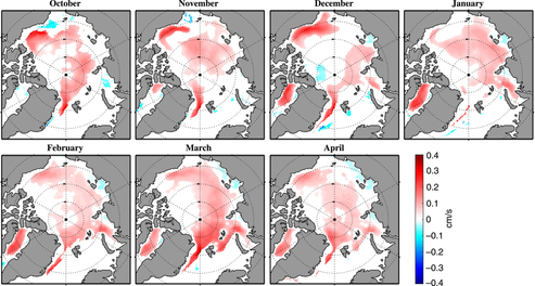
Negative trends in ice drift anomalies are observed for the month of October and November in the north of Alaska, where loss in sea-ice cover has resulted from ‘Arctic amplification’ (Serreze, Barrett, Stroeve, Kindig, & Holland, Reference Serreze, Barrett, Stroeve, Kindig and Holland2009) as well as the later ice formation and freeze up (Fig. 6). Enhanced drift speeds occurred in the western periphery of BG during the period from October to December, which can be linked to a more mobile ice pack in that area. Positive trends during March correspond with the enhanced meridional drift. Figure 6 highlights that the trends are stronger in October–December for the Pacific Arctic. The results match with the findings of Petty et al. (Reference Petty, Hutchings, Richter-Menge and Tschudi2016) and Howell et al. (Reference Howell, Brady, Derksen and Kelly2016), which have shown that the seasonality of ice drift in the Beaufort has a peak in October.

Fig. 6. Statistically significant trends in the sea-ice drift speed anomalies for each month for winters 1979–2015. The trends shown are statistically significant, with P < 0.05.
Zonal ice drift anomalies are significant features in the western Beaufort Sea, suggesting enhanced anticyclonic circulation (Fig. 7a). These include northern Baffin Bay, suggesting enhanced eastward flow; north of Greenland, suggesting enhanced eastward drift; and through the Fram Strait, suggesting enhanced westward drift, which is consistent with the west–east pressure gradient defined by Van Angelen, Van den Broeke, & Kwok (Reference Van Angelen, Van den Broeke and Kwok2011) over the Fram Strait. In the context of trends in meridional drift anomalies, enhanced anticyclonic circulation is again confirmed in the eastern and western Beaufort Sea, in southward transport in the Fram Strait and in Baffin Bay. This suggests increased export to Baffin Bay from the Arctic and Canadian Archipelago. Enhanced poleward flow is observed in the Kara and Laptev Sea regions, which shows the strengthening of TPD over the time series.

Fig. 7. Trends in the sea-ice drift anomalies for the zonal (left) and meridional (right) component in winter. Negative trend values (in blue) show the east–west sea-ice motion whereas the positive values show the sea-ice motion in the west–east direction (in red). The negative values (shown in blue) in the meridional component show the north–south drift of the sea-ice as compared to the positive values (shown in red), which show the south–north sea-ice motion.
Summary and conclusions
Results obtained from the mean sea-ice drift patterns for 36 winters within the period 1979–2015 highlight the three primary circulation patterns in the mean sea-ice motion map in the central Arctic Ocean: (1) anticyclonic motion in the Canadian Basin, i.e. BG, (2) TPD, as documented in earlier studies, over the past several decades, and (3) a motion system in the Eurasian Basin moving ice from the Kara Sea via the ocean route between Franz Josef Land and Novaya Zemlya. The KS circulation regime is smaller in spatial scale and occurs independently of TPD. Kwok (Reference Kwok2000) defined Kara Sea as a net exporter of sea-ice, sometimes to the eastern Arctic Ocean and other times to the Barents Sea. The boundaries of these circulation features were defined from the 36-year mean winter ice drift map (Fig. 1). In particular, we reach the following conclusions regarding spatial variability in drift patterns:
1. The first three modes of EOF explain only half (52.4%) of the variance in the dataset, with 30.2%, 13.5 and 8.7% for modes one, two and three, respectively. The first three modes explain that only the first two patterns are consistent and the rest only last for one or two winters out of the record. The first EOF mode shows a pattern similar to the 36-year average winter pattern for the entire Arctic Basin. The second mode of EOF shows a cyclonic motion of the ice in the entire basin, while the third mode shows the drift of the ice towards the Bering Sea. The first three EOF modes highlight that the drift patterns are highly variable.
2. The winter drift patterns in 2005 and 2011 show an anticyclonic motion covering the entire basin; Serreze et al. (Reference Serreze, McLaren and Barry1989) defined such patterns as the short-term reversals in TPD but the change in the scale and frequency of such events can influence the ice flux through the Fram Strait. The sharp decline in September minimum sea-ice extent in 2007 and 2012 paired with the dominance of the BG in the basin can affect the freshwater budget of the Arctic Ocean.
3. It has been observed that ice motion in the Kara Sea is mainly via the ocean route between Franz Josef Land and Novaya Zemlya. Whereas in the winter seasons when an anticyclonic ice motion pattern covering the entire basin is observed, ice from KS merges with TPD, thus increasing ice export through the Fram Strait.
The temporal patterns in these circulation regimes were evaluated using trend analysis. In particular, our conclusions regarding the long-term trend in drift speeds are as follows:
1. The long-term trend in the anomalies in the sea-ice drift speeds from October 1979 to April 2015 shows that the trends are more pronounced in October–December for the Pacific Arctic (Fig. 6). Recent studies by Petty et al. (Reference Petty, Hutchings, Richter-Menge and Tschudi2016) and Howell et al. (Reference Howell, Brady, Derksen and Kelly2016) also show the seasonality of ice drift in the Beaufort has a peak in October. Rampal et al. (Reference Rampal, Weiss and Marsan2009) observed a substantial increase in the mean sea-ice drift speeds for the winter season (+17% per decade). Overall positive trends in the sea-ice drift speeds for winter have also been observed by Häkkinen et al. (Reference Häkkinen, Proshutinsky and Ashik2008), Kwok et al. (Reference Kwok, Spreen and Pang2013) and Spreen et al. (Reference Spreen, Kwok and Menemenlis2011).
2. The winter of 1997–1998 depicted the beginning of very high drift speeds for the first time (since 1979) in the region north of the Alaskan coast, with drift speeds of up to 10 cm/s, compared to drift speeds of up to 6 cm/s during 1979–1996 (Fig. S1).
3. The basin-wide 36-year trend in the mean winter ice drift anomalies shows the strengthening of the BG, TPD and the drift patterns emerging from the Kara Sea. Statistically, positive drift trends are observed in all three circulation patterns at the 95% confidence interval. An equally strong increasing trend is also observed for the ice drift along the western coast of Baffin Bay (Fig. 4a).
4. Non-significant trends are observed in MYI dominated areas. This suggests drift trends are related to the change in ice type and thickness from MYI towards FYI. The previous studies have also shown the continued net decrease in multiyear ice in the region north of the Canadian Archipelago (Maslanik et al., Reference Maslanik, Fowler, Stroeve, Drobot, Zwally, Yi and Emery2007, Reference Maslanik, Stroeve, Fowler and Emery2011). Non-significant trends are also associated with negative trends of generally weak drift speeds due to the presence of landfast ice.
Much of our study has rested on the analyses of the average winter sea-ice drift speeds, patterns and their inter-annual evolution from passive microwave satellite data (ftp://sidads.colorado.edu/pub/DATASETS/nsidc0116_icemotion_vectors_v3/data/north/means/). The significance of this study lies in the pursuit of a better understanding of the role sea-ice drift plays in the continually accelerating changes in the Arctic sea-ice cover. With the new thinner ice regime, old assumptions that pack ice drifts at about 2% of the surface wind speed with a deviation angle of 30–45° to the right of the surface winds in the Northern Hemisphere (Nansen, Reference Nansen1902) may not hold true and responses to forcing may not be valid as we move forward, indicating that past research needs to be updated. The results presented here suggest that the recent drift patterns have been affected by the conditions of thinner sea-ice. A logical extension of this work would be to examine the effect of such ongoing changes on the export of ice through the Fram Strait and Baffin Bay.
Supplementary material
To view supplementary material for this article, please visit https://doi.org/10.1017/S0032247418000566.
Author ORCIDs
Satwant Kaur 0000-0003-2814-1692
Acknowledgements
Polar Pathfinder Sea Ice Mean Monthly Motion Vectors (Version 3) data were provided by NSIDC. The data are available for academic purposes through the NSIDC Portal (https://nsidc.org/data/docs/daac/nsidc0116_icemotion.gd.html or ftp://sidads.colorado.edu/pub/DATASETS/nsidc0116_icemotion_vectors_v3/data/north/means/). Thanks to University of Manitoba Graduate Fellowship (UMGF) and Graduate Enhancement of Tri-Council Stipends (GETS). This is a contribution to the Arctic Science Partnership (ASP) and the ArcticNet Network of Centres of Excellence. Special thanks to Dr Jennifer V. Lukovich from University of Manitoba for all her support, encouragement and contribution to this work. Thanks also to two anonymous reviewers and the editor Trevor McIntyre for their helpful feedback.
Financial support
This work was supported by the Natural Sciences and Engineering Research Council of Canada through funds to DGB (grant number 317528-328005-2000).