Introduction
There is a growing interest in the survey of genetic diversity in wild relatives of cultivated crops due to their potential as sources of valuable agronomic and stress-tolerance traits. Among the wild species of immediate interest for tomato improvement is Solanum pimpinellifolium L. This species is considered to be the immediate ancestor of cultivated tomato and hybridizes with it freely. It is native to Peru and Ecuador in Western South America, where it is found in dense populations located in undisturbed areas and adapted to diverse environmental conditions ranging from the coastal desert climate to the humid and foggy conditions of higher altitudes (Wiersema and León, Reference Wiersema and León1999; Zuriaga et al., Reference Zuriaga, Blanca, Cordero, Sifres, Blas-Cerdán, Morales and Nuez2009; USDA-ARS, 2011).
S. pimpinellifolium is of great importance to tomato breeding. It is a source of the disease-resistance genes to late blight caused by Phytophthora infestans (Mont.) de Bary (Ph-3) (Chunwongse et al., Reference Chunwongse, Chunwongse, Black and Hanson2002), Fusarium wilt caused by Fusarium oxysporum Schlechtend. f. sp. lycopersici W.C. Snyder & H.N. Hans. (I2) (Segal et al., Reference Segal, Sarfatti, Schaffer, Ori, Zamir and Fluhr1992) and bacterial speck caused by Pseudomonas syringae pv. tomato (Pto) (Martin et al., Reference Martin, Williams and Tanksley1991) which are routinely being used in breeding programmes employing marker assisted selection. Furthermore, this species has also been employed for the investigation of the genetic control of traits such as fruit shape and size (van der Knaap et al., Reference van der Knaap, Sanyal, Jackson and Tanksley2004).
Likewise, this species has been accorded special significance in the research and breeding portfolio of AVRDC – The World Vegetable Center. A thorough analysis of the genetic diversity and structure of the germplasm accessions in a given species is a fundamental requirement for the effective use of this material for breeding and crop improvement. An understanding of the population structure in a given panel is also necessary for successful association studies. The presence of population structure within an association mapping population can be an obstacle to the application of association analysis as it often generates spurious genotype–phenotype associations (Thornsberry et al., Reference Thornsberry, Goodman, Doebley, Kresovich, Nielsen and Buckler2001; Yu and Buckler, Reference Yu and Buckler2006; Zhu et al., Reference Zhu, Gore, Buckler and Yu2008). Though both single nucleotide polymorphism (SNP) and simple sequence repeat (SSR) markers are used for evaluating genetic diversity and population structure, SSRs are preferred because they offer the potential to detect multiple alleles compared to SNPs, which are biallelic and hence less informative per locus (Remington et al., Reference Remington, Thornsberry, Matsuola, Wilson, Whitt, Doebley, Kresovich, Goodman and Buckler2001).
Caicedo and Schaal (Reference Caicedo and Schaal2004) investigated the population structure in 16 populations of S. pimpinellifolium collected from the northern part of Peru based on an intron sequence of the Vac gene. Zuriaga et al. (Reference Zuriaga, Blanca, Cordero, Sifres, Blas-Cerdán, Morales and Nuez2009) studied the genetic and bioclimatic variation in this species using 10 microsatellite markers. However, to our knowledge, no earlier study examined the population structure of S. pimpinellifolium germplasm using genome-wide SSR markers.
Core collections are an expeditious means to intensively characterize, explore and use crop genetic resources stored in genebanks as well as to monitor genetic drift during preservation and identify gaps in the genetic diversity of the crop for further collecting and complementing the germplasm collection (Frankel and Brown, Reference Frankel, Brown, Holden and Williams1984). Several strategies have been employed to form core collections that maximize the diversity contained in the original collection. Stratified random sampling was found to be better than simple random sampling (Balfourier et al., Reference Balfourier, Charmet, Prosperi, Goulard and Monestiez1998; Hu et al., Reference Hu, Zhu and Xu2000; Chandra et al., Reference Chandra, Huaman, Hari Krishna and Ortiz2002; Franco et al., Reference Franco, Crossa, Warburton and Taba2006). When using molecular markers to determine a core for the retention of genetic diversity, the maximization (M) strategy has been implemented in the software program MSTRAT (Gouesnard et al., Reference Gouesnard, Dallard, Bertin, Boyat and Charcosset2005) and PowerCore (Kim et al., Reference Kim, Chung, Cho, Ma, Chandrabalan, Gwag, Kim, Cho and Park2007). The PowerCore program has the capacity to represent all alleles identified by molecular markers and classes of phenotypic observations by means of an advanced M strategy, implemented through a modified heuristic algorithm. It was found to be the most efficient strategy for the development of a core collection (Kim et al., Reference Kim, Chung, Cho, Ma, Chandrabalan, Gwag, Kim, Cho and Park2007; Agrama et al., Reference Agrama, Yan, Lee, Fjellstrom, Chen, Jia and McClung2009; Moe et al., Reference Moe, Gwag and Park2011).
The objectives of the present study were to (1) examine the population structure of the S. pimpinellifolium collection maintained by AVRDC – The World Vegetable Center and (2) construct a core set of AVRDC's S. pimpinellifolium collection.
Materials and methods
Plant materials
AVRDC – The World Vegetable Center – maintains 322 accessions of S. pimpinellifolium (AVRDC Vegetable Genetic Resources Information System (AVGRIS), 2011). From this collection, 190 accessions or approximately 60% of the total collection, representing 14 countries (one accession with an unknown origin) were selected for the present study, based on the AVGRIS passport data. Details of the accessions used in this study are shown in Supplementary Table S1 (available online only at http://journals.cambridge.org). For the accessions numbered 36, 43–47, 154 and 155, the indicated origin ‘USA’ is questionable as, although the material was donated from a source within the USA (in some cases, from a breeding company), no collecting information on the country of origin is available (Supplementary Table S1, available online only at http://journals.cambridge.org). It is likely that the original material was collected in South America. The 190 accession panel included 33 out of 40 accessions designated as S. pimpinellifolium core by the Tomato Genetics Resource Center (TGRC; http://tgrc.ucdavis.edu/).
Several authors have reported that since S. pimpinellifolium and Solanum lycopersicum var. cerasiforme are sympatric, the morphological limits based on fruit size and leaf shape are fuzzy and there are genotypes with intermediate forms that cannot be clearly classified into either of the two species (Rick and Fobes, Reference Rick and Fobes1975; Rick et al., Reference Rick, Fobes and Holle1977; Ranc et al., Reference Ranc, Muños, Santoni and Mathilde2008). Two accessions, numbered 23 and 86, are of this kind and were also included in the study. Furthermore, the accession numbered 33 and included as S. pimpinellifolium in this study was originally collected as wild tomato material in Ecuador and donated to the United States Department of Agriculture – Agricultural Research Service (USDA-ARS) in 1939. It was received by the AVRDC genebank from USDA-ARS as S. pimpinellifolium accession, but had its nomenclature changed to Solanum section lycopersicum hybrid in the GRIN database in September 2008 (http://www.ars-grin.gov/cgi-bin/npgs/acc/search.pl?accid=133542).
SSR genotyping
All accessions were grown under greenhouse conditions and leaf samples from one representative plant per accession were collected for deoxyribonucleic acid extraction. The 190 accessions were genotyped at 48 SSR loci which are available at the online resource of the Solanaceae genome network (Frary et al., Reference Frary, Xu, Liu, Mitchell, Tedeschi and Tanksley2005; solgenomics.net). Markers were selected to ensure an even distribution on the genome with an average distance between markers of approx 20 cM, satisfying the no-linkage assumption for structure analysis. The methodology of genotyping used in this study is described by Geethanjali et al. (Reference Geethanjali, Kadirvel, de la Peña, Rao and Wang2011). Information on primer sequences and polymerase chain reaction amplification conditions for each set of primers are available at solgenomics.net.
Statistical analysis
The genetic diversity measures included the major allele frequency, the average number of alleles, observed heterozygosity (H o), gene diversity (expected heterozygosity; H e) and polymorphism information content (PIC). Computations were conducted using the software program PowerMarker version 3.25 (Liu and Muse, Reference Liu and Muse2005).
Estimating the population structure
The genotypic data for 48 SSR markers were analyzed by employing a model-based approach available in Structure 2.3.3 program to subdivide the original population into different sub-populations (Pritchard et al., Reference Pritchard, Stephens and Donnelly2000). The membership of each genotype was tested from K = 1 to K = 10 (K = putative number of populations) with the admixture model, along with a burn-in of 50,000, run length of 100,000 and a model allowing for admixture and correlated frequencies with prior information on their origin. Because the estimated log-probability of data [LnP(D)] from Structure over-estimates the number of sub-populations, we used the delta K measure to estimate the number of sub-populations (Evanno et al., Reference Evanno, Regnaut and Goudet2005). This was carried out using the online version of Structure harvester (http://tayloro.biologyucla.edu/Struct_harvest). The results of the five replicate runs from Structure were integrated by CLUMPP software (Jakobsson and Rosenberg, Reference Jakobsson and Rosenberg2007).
The run of the estimated numbers of sub-populations showing maximum likelihood was used to assign accessions with membership probabilities ≥ 0.75 to subgroups. Accessions with membership probabilities less than 0.75 were assigned to an admixture group (Stich et al., Reference Stich, Melchinger, Frisch, Maurer, Heckenberger and Reif2005). Thus, identified sub-populations were further subdivided using separate runs of Structure as proposed by Pritchard and Wen (Reference Pritchard and Wen2004).
To investigate population differentiation, an analysis of molecular variance (AMOVA) and estimation of pairwise F statistics (F st) among populations was performed using PowerMarker version 3.25 (Liu and Muse, Reference Liu and Muse2005).
Development of a core set
The advanced M strategy, based on a modified heuristic algorithm implemented in the PowerCore software by Kim et al. (Reference Kim, Chung, Cho, Ma, Chandrabalan, Gwag, Kim, Cho and Park2007), was used to develop the core set. Sampling the original collection of 322 accessions was performed with an effort to maximize both, observed alleles at SSR loci and the number of phenotypic trait classes. Data of 32 qualitative and 22 quantitative phenotypic traits and 48 SSR markers generated from 190 accessions of S. pimpinellifolium were used to develop the core set.
The phenotypic traits were recorded according to the AVRDC–GRSU Characterization Record Sheet (unpublished data). Most of these traits are consistent with the IPGRI descriptor list for tomato (IPGRI, 1996), but the scales of some of the IPGRI descriptors have been modified and a few descriptors have been added. The IPGRI descriptor codes are indicated in brackets, where applicable. Each code in the rating scale of the qualitative phenotypic traits was defined as a class. The qualitative phenotypic traits used in this study were recorded during different growth stages as follows: (1) seedling data: anthocyanin coloration of hypocotyl, hypocotyl pubescence (7.1.1.3); (2) plant vegetative data: plant growth type (7.1.2.1), leaf attitude (7.1.2.8), leaf type (7.1.2.9), degree of leaf dissection (7.1.2.10), anthocyanin coloration of leaf veins (7.1.2.11); (3) inflorescence and fruit: inflorescence type (7.2.1.1), style position (7.2.1.7), fruit size homogeneity (7.2.2.7), predominant fruit shape (7.2.2.5), exterior colour of immature fruit (7.2.2.1), intensity of greenback (7.2.2.3), presence of jointless pedicel (7.2.2.20), ribbing at calyx end (7.2.2.14), fruit firmness (7.2.2.35), radial cracking (8.2.3), concentric cracking (8.2.4), fruit fasciation (8.2.5), exterior colour of mature fruit (7.2.2.11), fruit shoulder shape (7.2.2.16), shape of pistil scar (7.2.2.32), fruit blossom end shape (7.2.2.33), blossom end scar condition (7.2.2.34), flesh colour of pericarp (7.2.2.26), flesh colour intensity (7.2.2.27), fruit cross-sectional shape (7.2.2.29), vascular bundle content (8.2.6), colour of core (7.2.2.28), puffiness appearance (8.2.9), skin colour of ripe fruit (7.2.2.23), and easiness of skin peeling (7.2.2.22).
Similarly, an interval was defined to separate the full range of measurements and establish classes for 22 quantitative phenotypic traits, viz. primary leaf length (7.1.1.4), primary leaf width (7.1.1.5), number of leaves under first inflorescence (7.1.2.7), number of days to flowering (8.1.1), number of flowers per inflorescence (8.1.5), petal length (7.2.1.5), sepal length (7.2.1.6), stamen length (7.2.1.10), number of days to fruiting, number of fruit set per inflorescence (8.1.6), fruit weight (7.2.2.8), fruit length (7.2.2.9), fruit width (7.2.2.10), pedicel length (7.2.2.17), width of pedicel scar (7.2.2.20), size of corky area around pedicel scar (7.2.2.21), thickness of fruit wall (7.2.2.24), number of locules (7.2.2.31), thickness of pericarp (7.2.2.25), size of core (7.2.2.30), length of pedicel scar, and soluble solids (8.3.1). These variables were automatically classified into different classes by the PowerCore program based on Sturges' rule (k = 1+Log2(n), where k is the number of bins and n is the number of observed accessions).
The resulting core was compared with the original collection to assess its homogeneity. Nei's gene diversity index (Nei, Reference Nei1973) and the Shannon Weaver diversity index (Shannon and Weaver, Reference Shannon and Weaver1963) were estimated for each of the SSR markers and phenotypic traits in both the core and the original collection. Homogeneity was further evaluated in terms of mean difference (MD%), variance difference (VD%), coincidence rate of range (CR%) and variable rate of coefficient of variance (VR%). Coverage of all the phenotypic traits in the original collection was estimated in the core as proposed by Kim et al. (Reference Kim, Chung, Cho, Ma, Chandrabalan, Gwag, Kim, Cho and Park2007)
where D c is the number of classes occupied in the core set, D e is the number of classes occupied in the original collection for each trait and m is the number of traits.
Results
Basic statistics
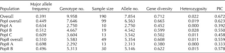
A total of 377 alleles were detected with an average of 7.85 alleles per locus and a range of 2 (SSR80) to 18 (SSR69) alleles per locus (Supplementary Table S2, available online only at http://journals.cambridge.org). Out of this total, 52 alleles at 28 loci were extremely rare-frequency alleles ( < 1% frequency). Gene diversity and PIC over the whole panel were 0.712 and 0.672, respectively. The mean heterozygosity was 2.22%.
Population structure
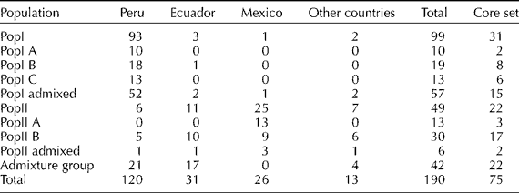
A total of 48 SSR markers were used to understand the population structure in the panel of 190 accessions of S. pimpinellifolium employing a model-based approach of Structure. Fifty data sets were obtained by setting the number of possible clusters (K) from 1 to 10 with five replications each. The results were then permuted for each K value using CLUMPP software. The LnP(D) value for each given K increased with the increase of K, but since there was no abrupt change in LnP(D), the probable K value could not be inferred (Fig. 1(a)). However, applying the second-order statistics (ΔK) developed by Evanno et al. (Reference Evanno, Regnaut and Goudet2005), there was a sharp peak of ΔK at K = 2, suggesting two major populations (Fig. 1(b)). A similar pattern was reported by Ranc et al. (Reference Ranc, Muños, Santoni and Mathilde2008). The first group, Population I (PopI), included 99 accessions, 93 of which originated from Peru (Table 1). The second group, Population II (PopII), contained 49 accessions which predominantly came from Mexico (25 accessions) and Ecuador (11 accessions). The remaining 42 genotypes had membership probabilities lower than 0.75 in any group and were classified into an admixture group. This group included 17 lines from Ecuador and 21 lines from Peru.

Fig. 1 Two different methods for determining optimal value of K: (a) the ad hoc procedure described by Pritchard et al. (Reference Pritchard, Stephens and Donnelly2000); (b) the second-order statistics (ΔK) developed by Evanno et al. (Reference Evanno, Regnaut and Goudet2005), for the full germplasm set (a colour version of this figure can be found online at journals.cambridge.org/pgr).
Table 1 Classification of 190 accessions of a Solanum pimpinellifolium germplasm panel into sub-populations, their respective countries of origin and number of accessions from each sub-population selected into the core set

The two main populations were further subdivided into five subgroups. The ΔK values suggested K = 3 in PopI (Supplementary Fig. S1, available online only at http://journals.cambridge.org) and K = 2 in PopII (Supplementary Fig. S2, available online only at http://journals.cambridge.org). PopI included three subgroups, viz. PopI A with 10 lines, PopI B with 19 lines, PopI C with 13 lines and an admixed group consisting of 57 lines (Table 1; Fig. 2).

Fig. 2 Model-based cluster membership of 190 accessions in two main groups and five subgroups (a colour version of this figure can be found online at journals.cambridge.org/pgr).
PopII was classified into two subgroups. PopII A consisted of 13 accessions, all from Mexico. PopII B consisted of 30 accessions including 10 from Ecuador, nine from Mexico, five from Peru and six from other countries. PopII admixture included six lines with membership probabilities less than 0.75 in any of the two groups (Table 1).
PopI A included accessions collected in the regions between 12°10′S and 13°15′S latitudes corresponding to southern Peru. PopI B included accessions collected in the regions between 3°99′S and 8°6′S latitudes corresponding to northern Peru. PopI C included accessions collected mostly in the regions between 11°28′S and 12°8′S latitudes corresponding to central Peru. PopII A included accessions collected from Mexico and PopII B included accessions collected mostly in the regions between 0°52′S and 2°44′S latitudes corresponding to Ecuador.
Population differentiation
Comparing PopI and PopII, AMOVA results indicated that only 9.87% of the total genetic variation was partitioned among groups, 89.13% within groups and 1.0% within lines. Analysis with subgroups revealed that 78.05% of the variation occurred between subgroups and 21.95% within subgroups.
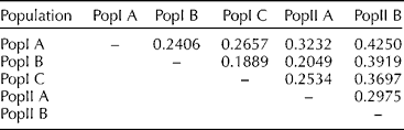
The pairwise comparison on the basis of values of F st may be interpreted as standardized population distances between two populations. The pairwise F st value in this study ranged from 0.189 between PopI B and PopI C to 0.425 between PopI A and PopII B, with an average pairwise F st of 0.296 (Table 2).
Table 2 Pairwise F st estimates among the five sub-populations identified
Genetic diversity of sub-populations
The genetic diversity for each population and sub-population was assessed (Table 3). Accessions in PopI coming predominantly from Peru (Table 1) were more diverse with a higher mean allele number of 6.563 and gene diversity of 0.665 compared with the accessions of PopII which predominantly came from Mexico and Ecuador (Tables 1 and 3). Among this Peruvian group (PopI), PopI A corresponding to individuals from southern Peru exhibited the least diversity in terms of allele number (2.750) and gene diversity (0.452) (Table 3). This group also exhibited the least heterozygosity (0.00). A gradual increase in these diversity measures and the heterozygosity was observed from southern Peru (PopI A) via central Peru (PopI C) to northern Peru (PopI B). Within the subgroups of PopI, PopI B exhibited the highest allele number (4.542) and gene diversity (0.599). This group also exhibited the highest heterozygosity (0.028) compared to any other subgroup. The geographically contiguous Ecuadorian subgroup (PopII B), though quite differentiated from the northern Peru group (PopI B), exhibited similar levels of diversity in terms of allele number (5.146) and gene diversity (0.622). PopII A, with accessions coming exclusively from Mexico, exhibited the least diversity among all subgroups in terms of allele number (2.313) and gene diversity (0.380) along with the least heterozygosity (0.00).
Table 3 Genetic diversity of the five sub-populations based on 48 SSR markers

Core set
The 190 accessions of S. pimpinellifolium originated from 14 countries, the majority of which came from Peru (120), followed by Ecuador (31) and Mexico (26). The accessions from these three countries accounted for 93.68% of the total collection. The subset of 190 accessions included 33 out of the 40 accessions designated as S. pimpinellifolium core by TGRC (http://tgrc.ucdavis.edu/).
On the basis of 32 qualitative and 22 quantitative phenotypic traits and 48 SSR markers, the heuristic search identified 75 accessions covering seven countries from the original subset of 190 accessions originating from 14 countries. The MD%, VD%, CR% and VR% are designed to comparably evaluate the property of a core collection with its initial collection (Agrama et al., Reference Agrama, Yan, Lee, Fjellstrom, Chen, Jia and McClung2009). The resultant core of this study had a MD of 11.35%, a VD of 33.93%, a VR of 110.75% and a CR of 99.14% with the original collection. The VR% exceeds 100%, indicating good representation of the original collection. The CR% was much higher than the 80% threshold suggested by Kim et al. (Reference Kim, Chung, Cho, Ma, Chandrabalan, Gwag, Kim, Cho and Park2007), indicating a homogeneous distribution.
Both the original and core collection had the same total number of polymorphic alleles produced by 48 markers. The distributions of the Nei gene indices and Shannon Weaver diversity indices were similar between the core and original collections. The base collection had an average Nei diversity index of 0.74 with a minimum of 0.312 for SSR112 and a maximum of 0.91 for SSR69 over the 48 markers. The diversity index averaged 0.75 in the core set with a minimum of 0.29 for SSR112 and a maximum of 0.90 for SSR69. Similarly, the base collection had an average Shannon Weaver diversity index of 1.48 with a minimum of 0.571 for SSR346 and a maximum of 2.398 for SSR69 over the 48 markers. The diversity index averaged 1.53 in the core set with a minimum of 0.61 for SSR112 and a maximum of 2.535 for tom184. The minor differences in average diversity indices between the base and core collections were not statistically significant. More than 91% of the markers had a Nei's diversity index higher than 60%, indicating a high diversity across the markers (Fig. 3). The calculated coverage value for the resulting core was 100%, suggesting that there is full coverage of all the diversity present in each class of phenotypic and molecular traits.

Fig. 3 Distribution of Shannon Weaver and Nei diversity indices among 48 SSR markers in the entire collection (E-SW; E-Nei) and the core collection (C-SW; C-Nei), compared with 33 accessions of TGRC core (TGRC-SW; TGRC-Nei). The markers have been placed according to their respective position within the tomato genome.
Discussion
The assessment of genetic diversity and structure of a germplasm panel is essential for the efficient organization of breeding material as well as the use of genetic resources for crop improvement (Fernie et al., Reference Fernie, Tadmor and Zamir2006; Li et al., Reference Li, Schulz and Stich2010). The use of SSR markers to interpret population structure results in much greater resolution due to higher polymorphism and tracking of recent population structures as a result of greater levels of linkage disequilibrium (LD) between SSR markers than with SNP markers which are considered to be evolutionarily older (Remington et al., Reference Remington, Thornsberry, Matsuola, Wilson, Whitt, Doebley, Kresovich, Goodman and Buckler2001; Flint-Garcia et al., Reference Flint-Garcia, Thornsberry and Buckler2003). SSR markers have been used to characterize population structure in maize (Remington et al., Reference Remington, Thornsberry, Matsuola, Wilson, Whitt, Doebley, Kresovich, Goodman and Buckler2001; Flint-Garcia et al., Reference Flint-Garcia, Thuillet, Yu, Pressoir, Romero, Mitchell, Doebley, Kresovich, Goodman and Buckler2005), rice (Flint-Garcia et al., Reference Flint-Garcia, Thornsberry and Buckler2003; Agrama et al., Reference Agrama, Eizenga and Yan2007) and other crops.
The population structure analysis identified two main and five sub-populations. Values of F st among the five sub-populations were significant, suggesting a real difference between these populations. However, several accessions had partial ancestry in more than one background. These accessions probably had a complex history involving intercrossing.
It was interesting to note that the first STRUCTURE analysis with all 190 accessions could not detect the five sub-populations. However, the sequential STRUCTURE analysis (Yang et al., Reference Yang, Yan, Shah, Warburton, Li, Li, Gao, Chai, Fu, Zhou, Xu, Bai, Meng, Zheng and Li2010) with the subsets of accessions detected those sub-populations and this result was supported by the pairwise estimates of F st. Although the current result is a fair indication of the presence of five subgroups, Evanno et al. (Reference Evanno, Regnaut and Goudet2005) suggest that a small number of loci and partial sampling of individuals can fail to detect the correct number of groups by STRUCTURE.
A clear differentiation was observed among populations based on geography. Peruvian accessions were genetically quite differentiated from the remaining accessions originating in Ecuador and Mexico. A possible cause of this differentiation could be the non-uniform nature of the coastal Ecuador and Peruvian climates, as suggested by Zuriaga et al. (Reference Zuriaga, Blanca, Cordero, Sifres, Blas-Cerdán, Morales and Nuez2009).
The highest heterozygosity was found in northern Peru (PopI B) and Ecuador (PopII B) subgroups and the lowest in southern Peru (PopI A) and Mexico (PopII A) subgroups. This low heterozygosity in southern Peru corroborates previous observations by other authors (Rick et al., Reference Rick, Fobes and Holle1977; Caicedo and Schaal, Reference Caicedo and Schaal2004; Zuriaga et al., Reference Zuriaga, Blanca, Cordero, Sifres, Blas-Cerdán, Morales and Nuez2009).
Based on the geographical pattern of sequence variation from the nuclear gene of 16 S. pimpinellifolium populations which originated from northern Peru, Caicedo and Schaal (Reference Caicedo and Schaal2004) concluded that northern Peru is the centre of origin of this species and that from this centre a gradual colonization took place along the Pacific coast. The present study, based on genome-wide SSR markers and a larger germplasm panel covering a much wider geographical area, confirms these results. The data suggest a northern Peruvian origin of this species which later migrated to Ecuador in the north and central to southern Peru in the south. The Ecuadorian group later migrated further north towards Mexico. A similar model was proposed by Zuriaga et al. (Reference Zuriaga, Blanca, Cordero, Sifres, Blas-Cerdán, Morales and Nuez2009). They opined that this migration must have caused a bottleneck and a loss of diversity, resulting in the selection towards autogamy in the new geographical regions which reduced the effective population size, heterozygosity and genetic diversity.
Employing PowerCore with its advanced M strategy, we developed a core set containing 75 accessions representing 39.47% of the selected germplasm panel (190 accessions) and 23.36% of the entire S. pimpinellifolium collection held at AVRDC (322 accessions). This is a higher percentage than the core sizes of cultivated crops which usually are in the range of 10% (Agrama et al., Reference Agrama, Yan, Lee, Fjellstrom, Chen, Jia and McClung2009). This can be accounted for by two reasons. First, this is a thematic core for a wild species with a small base panel resulting in a higher core percentage. Secondly, the accessions have been collected from the wild without human selection and breeding intervention; and Zhao et al. (Reference Zhao, Cho, Ma, Chung, Gwag and Park2010) noted that accessions of wild species or landraces possess greater allelic richness than the bred accessions, resulting in a larger core size while ensuring 100% allele coverage.
Core collections with low MD% and VD% and high VR% and CR% are considered to provide a good representation of the genetic diversity of the initial collection (Hu et al., Reference Hu, Zhu and Xu2000; Kim et al., Reference Kim, Chung, Cho, Ma, Chandrabalan, Gwag, Kim, Cho and Park2007; Agrama et al., Reference Agrama, Yan, Lee, Fjellstrom, Chen, Jia and McClung2009). The MD% of 11.35% and VD% of 33.93% observed in this study are less than those observed in rice (Kim et al., Reference Kim, Chung, Cho, Ma, Chandrabalan, Gwag, Kim, Cho and Park2007; Agrama et al., Reference Agrama, Yan, Lee, Fjellstrom, Chen, Jia and McClung2009) and cotton (Hu et al., Reference Hu, Zhu and Xu2000). Similarly, the VR% (110.75%) and CR% (99.14%) are similar to the values obtained in the above experiments. Therefore, this core may be considered as a sound representation of S. pimpinellifolium genetic diversity found in the AVRDC genebank.
The constitution of the original collection included 99 accessions from PopI, 49 from PopII and 42 from Admixture which had a skewed representation towards PopI. However, the core set has a balanced representation including 31 accessions from PopI, 22 from PopII and 22 from Admixture. Similarly, the constitution of the original collection included 120 accessions from Peru, 31 from Ecuador, 26 from Mexico and 13 from other countries. The developed core set consists of 40 accessions from Peru, 17 from Ecuador, 14 from Mexico and 4 from other countries. Thus, the proposed core has a balanced representation of both populations and geographic origins.
The developed core exhibits improved genetic diversity in terms of mean allele number (7.56), Shannon Weaver index (1.53) and Nei's index (0.75) compared to TGRC's core with a mean allele number of 5.58, Shannon Weaver index of 1.30 and Nei's index of 0.67 (Fig. 3). Further, out of 33 TGRC designated core accessions, only eight accessions could be selected into the core set of the present study constituting 10.66% of the total core size. This suggests that the core set developed in this study possesses greater diversity. However, a core is a dynamic concept, whose constitution keeps changing with greater germplasm explorations coupled with genotypic and phenotypic assays. In the present case, Ecuador, in spite of its high genetic diversity and being quite differentiated from the Peruvian group, is under-represented in most genebanks. Hence, future explorations in this country can possibly add novel variation.
The core set of S. pimpinellifolium identified in this study is very useful for tomato breeders. This species has proved to be a good source of alleles for biotic stress tolerance (Foolad, Reference Foolad2007). Considering that the natural range of S. pimpinellifolium encompasses environments as diverse as the Ecuadorian tropical forest and the coastal Peruvian desert, this species is also a potential source of beneficial alleles for abiotic stress tolerance.
Understanding the population structure is a prerequisite for future studies aimed at association mapping where regions of the genome can be associated with phenotypes of interest. The choice of germplasm for association mapping is key to the success of association analysis (Flint-Garcia et al., Reference Flint-Garcia, Thornsberry and Buckler2003; Yu and Buckler, Reference Yu and Buckler2006; Zhu et al., Reference Zhu, Gore, Buckler and Yu2008). Ideally, an association panel should contain the maximum amount of genetic diversity, as it is often required to resolve complex trait variation to the level of a single gene or nucleotide (Yang et al., Reference Yang, Yan, Shah, Warburton, Li, Li, Gao, Chai, Fu, Zhou, Xu, Bai, Meng, Zheng and Li2010). The use of a core collection allows the study of maximum diversity in a reduced number of accessions, which in turn increases the probability of detecting variants of interest in association studies which involve complex traits. Knowledge gained through the use of a core collection allows the choice of optimal crosses for generating suitable mapping populations (Agrama et al., Reference Agrama, Yan, Lee, Fjellstrom, Chen, Jia and McClung2009).