

1. Introduction
As a fact of social reality, polarization seems ubiquitous and all too easy to produce. Any small room filled with enough people and any remotely contentious issue seems to suffice to create polarization between rival factions. As a fact of modeling, however, it proves surprisingly difficult to produce a model in which simple and intuitive mechanisms produce patterns that even roughly resemble familiar patterns of polarization. Imitation and the influence of social contacts are an obvious and ubiquitous aspect of opinion dynamics, but as early as 1964 Robert Abelson noted that models in which agents imitate the opinions of others seem to tend inevitably toward central convergence. Abelson points out one way computational models often fail: “Since universal ultimate agreement is an ubiquitous outcome of a very broad class of mathematical models, we are naturally led to inquire what on earth one must assume in order to generate the bimodal outcome of community cleavage studies” (Reference Abelson1964, 153). Another way that simple computational models can fail is by producing bifurcation that under iteration progressively drives all agents from middle values to the extremes at 0 and 1. Neither inevitable movement toward a central consensus nor inevitable movement to full polarized extremes seems characteristic of social polarization as we know it.
It has been repeatedly emphasized that models are constructed for many purposes. Point predictions and a detailed mirroring of a complex reality are typically not the point and are not at any rate to be expected from simplified formal models (Epstein and Axtell Reference Epstein and Axtell1996; Epstein Reference Epstein2006, Reference Epstein2008; Epstein et al. Reference Epstein, Lemon, Hamberg, Sparling, Choffnes and Mack2007; Miller, Page, and LeBaron Reference Miller, Page and LeBaron2008; Grim et al. Reference Grim, Rosenberger, Rosenfeld, Anderson and Eason2013). It is often said of physical phenomena, for example, that it is simple models constructed in terms of spheres moving without friction on perfect planes that offers the clearest explanation and most fundamental understanding. The challenge for models of polarization that we pursue here, however, is in achieving even such a basic explanatory model and simple fundamental understanding. The question is not whether the simple computational models currently available for opinion polarization offer a realistic portrayal of empirical phenomena. The question we pursue here is whether available computational models suffice to capture, even roughly, plausible underlying mechanisms.
In what follows we consider the major families of models for social phenomena that have been appealed to as offering clues to the central mechanisms of polarization. Axelrod’s Cultural Diffusion and Polarization models represent one modeling tradition (Axelrod Reference Axelrod1997; Klemm et al. Reference Klemm, Eguiluz, Toral and Miguel2005; Flache and Macy Reference Flache and Macy2006a; Centola et al. Reference Centola, Gonzalez-Avella, Eguiluz and Miguel2007). The Hegselmann-Krause Bounded Confidence model and Deffuant’s Relative Agreement model define another approach (Deffuant et al. Reference Deffuant, Amblard, Weisbuch and Faure2002; Hegselmann and Krause Reference Hegselmann and Krause2002; Deffuant Reference Deffuant2006). Models in a Structural Balance tradition constitute a third family (Heider Reference Heider1946; Cartwright and Harary Reference Cartwright and Harary1956; Harary Reference Harary1959; Macy et al. Reference Macy, Kitts, Flache and Benard2003; Klemm et al. Reference Klemm, Eguiluz, Toral and Miguel2005; Kitts Reference Kitts2006). We extend the analysis to mechanisms for ‘group polarization’ suggested within social psychological theories of self-categorization (Lord, Ross, and Lepper Reference Lord, Ross and Lepper1979; Hogg, Turner, and Davidson Reference Hogg, Turner and Davidson1990). Each of the models analyzed purports to capture polarization, but it is clear that both the kinds and the patterns of phenomena they generate vary widely. We want to frame the behaviors of these disparate models in a way that allows us to evaluate and compare their abilities to capture plausible mechanisms for polarization of various kinds in various patterns.
In order to evaluate these models, however, we first need to understand the explanatory target. Precisely what opinion configurations count as polarized? What social dynamics qualify as dynamics of polarization? ‘Polarization’, it turns out, designates not a single unambiguous concept but a blurred cluster of concepts and measures. A range of very different social configurations and very different social dynamics have been lumped together under the term ‘polarization’. For some of these, a particular class of models may be appropriate. For others it may not. How well a model represents an explanatory mechanism for polarization therefore depends on what sense of polarization is at issue. The explanations offered by different models may not in fact be in competition because the explanans differs: it is different notions of polarization that the models are attempting to explain.
We begin, therefore, by disentangling nine senses of polarization and briefly sketching appropriate formal measures for each.Footnote 1 That conceptual/methodological breakdown gives us the tools necessary to examine polarization models and ascertain the different senses of polarization that a particular model is capable or incapable of producing. We replace broad claims that a particular model mechanism increases or decreases polarization with a finer-tuned evaluation of model effects in terms of each of our nine senses. Because the nine senses we identify are not exhaustive, we also indicate when other senses are invoked. By providing a disambiguation of polarization into these distinct phenomena (and formalized measures for capturing them), we facilitate the evaluation of a models’ ability to clarify the relevant social dynamics and thus constitute a useful explanation for at least some aspects of polarization. In the end we conclude that better modeling, more finely attuned to the various senses of ‘polarization’, will be required for a genuine understanding of the quite different opinion dynamics that have been conflated under that term.
2. The Many Senses of ‘Polarization’
Common wisdom has it that American society is becoming increasingly polarized (Fiorina, Abrams, and Pope Reference Fiorina, Abrams and Pope2005; Brownstein Reference Brownstein2007; McCarty, Poole, and Rosenthal Reference McCarty, Poole and Rosenthal2008; Hetherington and Weiler Reference Hetherington and Weiler2009). There are measurable aspects of political reality that support that common wisdom. In 1980, only 43% of Americans polled said that they thought there were important differences between the parties. The figure is now 74%. In 1976, almost a third thought it did not make a difference who was president. That figure is now cut in half. Between 1969 and 1976, the Nixon and Ford years, the rate at which Republicans voted along party lines was about 65% in both the House and the Senate. The same was true of Democrats. Between 2001 and 2004, under George W. Bush, Republicans voted with their party 90% of the time. Democrats voted with their party 85% of the time (McCarty et al. Reference McCarty, Poole and Rosenthal2008).
But, this kind of political polarization is certainly not new. George Washington’s farewell address in 1796 emphasized the danger of factions: “One of the expedients of party to acquire influence … is to misrepresent the opinions and aims of other[s],” he said. The spirit of a party kindles animosity and “agitates the community with ill-founded jealousies and false alarms.” A year later, Thomas Jefferson complained that because of partisan polarization “men who have been intimate all their lives cross the streets to avoid meeting” (Forman Reference Forman1900, 69). That was in fact true of Jefferson and John Adams for most of their political lives.
It has been argued, however, that a focus on political polarization within the political elite obscures a stable or declining cultural polarization within the broader population. On most issues, public polarization has not increased between groups, regardless of what groups are being compared: the young and the old, men and women, the more and the less educated, different regions of the country, or different religious affiliations. On a number of points, polarization has clearly decreased. Racial integration was once fought vociferously by major portions of the population, but that is certainly not true now. Views on women’s roles in public life were once extremely contentious in ways that are now quite generally recognized as archaic. Support for the death penalty has fallen, while a consensus on crime has moved toward tougher enforcement. The issue of gay marriage is fast losing its polarizing edge. Those changes have generally operated in parallel across distinctions of age, gender, education, region, and religious affiliation (Fiorina et al. Reference Fiorina, Abrams and Pope2005).
Polarization is currently a topic of intense interest among social scientists, with analysis of congressional affiliation and voting patterns, sociological studies on popular attitudes, and laboratory studies on media influence and attitude change all in search of a better understanding of central mechanisms (Fiorina and Abrams Reference Fiorina and Abrams2008; Iyengar, Sood, and Lelkes Reference Iyengar, Sood and Lelkes2012; Ura and Ellis Reference Ura and Ellis2012; Druckman, Peterson, and Slothuus Reference Druckman, Peterson and Slothuus2013; Großer and Palfrey Reference Großer and Palfrey2013; Lauderdale Reference Lauderdale2013; Levendusky Reference Levendusky2013; Prior Reference Prior2013; Leeper Reference Leeper2014; Thomsen Reference Thomsen2014; Weinschenk Reference Weinschenk2014; Mason Reference Mason2015). Claims regarding polarization, however, often remain frustratingly vague. However intuitive or intriguing those claims may be, it is often unclear what social phenomenon of belief configuration is at issue or in exactly what sense opinion has or has not become ‘polarized’. The problem is not restricted to popular presentations but appears in the technical literature of sociology, economics, and political science as well. Entire articles appear on polarization with little attempt to make it clear what precisely is meant by the term.
Greater clarity is demanded both in order to properly characterize social phenomena and in order to evaluate the models put forward as attempts to understand the basic social dynamics involved. For our study, as for others, it proves necessary to analyze different senses of ‘polarization’. We offer a starter set of nine senses. Formal measures appropriate to each are described briefly, with a more complete formal treatment left to a separate paper (Bramson et al. Reference Bramson, Grim, Singer, Fisher, Berger, Sack and Flocken2016).
We want to reiterate that the nine senses of ‘polarization’ outlined here are not exhaustive. For example, the term ‘polarization’ is sometimes used to refer to a static property (the population is polarized) and sometimes a process (the population is polarizing).Footnote 2 The formal measures we provide are properties of cardinal-valued belief distributions captured at time slices, which can be used to compare patterns of opinion on different issues or across different populations (static) or to compare changes across time in a single issue (process). There may be some senses of polarization that are intrinsically dynamic that cannot be captured by comparing time slices, but no senses of this type appear in the literature we have surveyed. For simplicity and clarity we focus on measures of beliefs (alternately: ideas, opinions, attitudes, etc.) distributed on a normalized spectrum along one dimension and use the simplest method for representing that distribution: a histogram of the number of individuals holding a specific belief. The concepts we outline have clear analogues in higher dimensions with modified measures, but higher dimensions also open up the possibility of further senses. Social networks, spatial distributions, and categorical data may call for further approaches, and we show how some of the same senses of polarization can be applied to those cases as well.
2.1. Polarization Type 1: Spread
An obvious way to measure polarization is in terms of the breadth of opinions; that is, how far apart are the extremes? DiMaggio, Evans, and Bryson call this ‘dispersion’: “the event that opinions are diverse, ‘far apart’ in content” (DiMaggio, Evans, and Bryson Reference DiMaggio, Evans and Bryson1996, 694). They also outline a dispersion principle: “Other things being equal, the more dispersed opinion becomes, the more difficult it will be for the political system to establish and maintain centrist political consensus” (693).
Polarization in the sense of spread can be measured as the value of the agent with the highest belief value minus the value of the agent with the lowest belief value (sometimes called the ‘range’ of the data). Polarization in the sense of spread is illustrated by the ends of the horizontal bar in figure 1. In higher dimensions it can be captured as the volume of the minimal bounding ellipsoid.

Figure 1. Belief distribution b shows greater polarization in the sense of spread than does belief distribution a. Two separate groups are shown, but that is irrelevant to polarization in the sense of spread.
Polarization in the sense of spread does not consider whether the agents with the minimum and maximum beliefs are extreme case outliers or the edges of large clusters. Spread is indicated in figure 1 using two groups (red and blue). But it should be emphasized that spread is a concept that applies to belief distribution across an entire population, rather than being group defined. Even if the minimum and maximum agents are representative of groups at the ends of the belief spectrum, spread will ignore that group characteristic just as it will ignore any groups in between. This lack of sensitivity to the shape of the distribution makes spread a weak measure of polarization in isolation, but it does capture the oft-reported feature of America political polarization that the extremists are getting more extreme while the overall shape is largely unchanged.
2.2. Polarization Type 2: Dispersion
Another simple way to measure polarization is statistical dispersion (or statistical variation). Unlike spread, which considers only the extremes of the population, dispersion considers only the overall shape of the distribution. Any of various measures of statistical dispersion might be used: mean difference, average absolute deviation, standard deviation, coefficient of variation, or entropy. Here we use average absolute deviation from the mean as a simple example. Polarization differences in the sense of dispersion are illustrated in figure 2. Note that the diagrams in the figure show dispersion increasing as spread is held constant. Like spread, dispersion is a measure across the distribution, without being tied to notions of groups or subpopulations. Note that this also matches dispersive polarization as defined in DiMaggio et al. (Reference DiMaggio, Evans and Bryson1996, 694)—“opinions are diverse, ‘far apart’ in content”—except that it considers all the beliefs rather than just the extremes.

Figure 2. Distribution c shows greater polarization in the sense of dispersion than does belief distribution b, which is greater than distribution a.
Although dispersion does not depend on any notion of groups, increasing the measure beyond a certain point on one dimension does require the formation of two modes in the distribution (as seen in fig. 2c). Bimodality is frequently mentioned as a feature of polarized distributions and sometimes as part of the definition (Fiorina et al. Reference Fiorina, Abrams and Pope2005). However, we can also find bimodality in distributions for other senses of polarization with specific value ranges. We revisit this point below.
2.3. Polarization Type 3: Coverage
The views of polarized factions are often thought of as constituting narrow and tightly packed sets of beliefs. A polarized society is thought of as one with little diversity of opinion, one in which only narrow bands of the opinion space are occupied. A simple way to envisage polarization in this sense is to think of the spectrum of possible beliefs as divided into small bins. The proportion of empty bins will then constitute a measure of polarization as coverage. That discrete measure, although simple, depends on the choice of bins: varying the width or location of bins can alter the measure for the same underlying data. A continuous variation is also possible by using halos of a given radius around each agent’s belief value and summing the lengths of empty space.
Figure 3 illustrates comparative polarization in the sense of coverage. Although it is not sensitive to either the shape of the distribution (e.g., whether occupied areas are close together or at the extremes) or the number of agents who hold each position, polarization in the sense of coverage does capture this basic feature of opinion diversity or variation. Furthermore, coverage works as a measure for categorical data—data for which the location on a spectrum is meaningless—and across any number of dimensions. Because it is a measure of diversity, with more diversity meaning less polarization, we can also apply more sophisticated diversity measures such as the inverse Simpson index to calculate coverage weighted by the number of agents holding the beliefs at issue (see Size Parity below).

Figure 3. Distribution a is more polarized than b in the sense of representing less coverage on the spectrum of potential belief. Although the plots show groups and differences in heights, neither of those features are aspects of polarization in the sense of coverage.
2.4. Polarization Type 4: Regionalization
Coverage represents how much of the belief spectrum is occupied by a society, without accounting for the pattern of areas occupied. ‘Polarization’ can also be used to indicate belief regionalization, without attending to the total area covered over all. In considering small bins of possible belief, for example, we might measure polarization not in terms of how many bins are filled but in terms of how many empty regions there are between filled areas. The area of uncovered opinion spaces corresponds directly to the concept of coverage. The number of uncovered intervals, in contrast, offers a distinct sense in which distributions can be polarized. Figure 4 shows two cases with the same coverage but in which counting empty regions between occupied areas gives us a measure of regionalization polarization in which b is more polarized than a.

Figure 4. Distributions with equal coverage but in which b shows a higher amount of polarization in the sense of regionalization because of a larger number of empty spaces between occupied areas.
Regionalization per se does not distinguish between a case (i) in which bins between 0 and 0.25 and between 0.35 and 0.60 are filled and a case (ii) in which bins between 0 and 0.25 and between 0.75 and 1 are filled; that is, the most basic notion of regionalization does not account for the widths of the gaps. For some cases, however, this may be the intuitive sense of polarization that we want. It can be combined with other measures to get a more refined description of a phenomenon at issue. Cases i and ii might be regionalized and have coverage to the same degree, for example, although the two groups in ii are farther apart in the sense of dispersion and the beliefs in ii also spread across a wider area.
Regionalization counts the completely distinct clusters in the distribution, related to but distinct from the number of groups (see below for polarization in the senses of both Distinctness and Groups). It does not have a simple, useful extrapolation to higher dimensions and cannot operate on categorical data. Finer-grained quantitative measures of group differences are presented below, but all of these depend on the a priori identification of groups within the data.
Defining Groups.—All of the polarization measures so far have been defined in terms of distribution characteristics observable from the whole population. No concept of groups is required for measures of polarization in terms of spread, dispersion, coverage, or regionalization. Other senses of polarization must be explicitly defined in terms of groups. One way to categorize groups is identify them directly from the histogram as collections of individuals categorized by the basins of attraction between local peaks. In this way groups are identified endogenously by the patterns in belief values, distinguishing unimodal from bimodal or trimodal distributions (Downey and Huffman Reference Downey and Huffman2001).
‘Polarization’ in various group-dependent senses is also used for cases in which groups are exogenously defined (e.g., by region, ethnicity, sex, education level, or other categories). Groups might also be defined in terms of network links representing association, influence, or communication. For example, one can first identify network-based groups using community structure algorithms, then use those collections of nodes as exogenously defined groups in order to break down the belief histogram. Exogenously defined groups may be those indicated by distinct colors in figure 5b. As the two panels of figure 5 make clear, exogenously defined groups may overlap in opinion, generating a very different picture than that indicated in the simpler opinion histogram of 5a. The important point is that the application of each of the group-dependent senses of ‘polarization’ below will depend on how the groups involved are identified.

Figure 5. For exogenously defined groups, the histogram for the entire population (a) may be broken into varying numbers of overlapping subpopulations, as in b.
2.5. Polarization Type 5: Community Fracturing
A first group-dependent sense of ‘polarization’ is community fracturing: the degree to which the population can be broken into subpopulations. Because different endogenous and different exogenous senses of ‘group’ will generate differing levels of community fracturing, this sense offers the level of polarization of the specified groups rather than of the population as a whole.
Figure 6 shows two belief distributions with groups endogenously defined using a local minima method: the distribution in 6b shows more groups than 6a. The population’s beliefs in the second case are more fragmented, indicating greater polarization in the sense of community fracturing. A population that moved dynamically from the first pattern to the second would be a community that showed increased polarization of its endogenously defined groups.

Figure 6. Polarization increases from a to b for endogenously defined groups.
In some applications groups can be exogenously defined; for example, one could have opinion data categorized by educational attainment level on the question of what percentage of the federal budget should be devoted to education. Distinct educational attainment groups could then be plotted together on the same belief spectrum. Defining groups endogenously and exogenously often/typically reveals different groupings of the beliefs. As illustrated in figure 7, aggregated communities may produce identical belief distributions overall yet show very different patterns of polarization in terms of endogenously defined a and exogenously defined b groups.

Figure 7. Polarization as network fracturing. Although overall histograms are identical, categorization in terms of networks may reveal either limited (a) or greater (b) group polarization.
Whether groups in the distribution of beliefs are endogenously or exogenously defined, community fracturing as a measure of polarization is about the number of groups. If agents are connected via a network structure, however, subcommunities may be referred to as ‘polarized’ simply in the sense that there is little or no communication between them. A similar phenomenon occurs in spatial models in which the locations of agents, or clusters of agents, are far apart. Such phenomena can be better thought of as separation and segregation: features that may produce or reflect polarized beliefs and that are also quantified by the number of groups but are not themselves senses of opinion polarization because they are not features of belief distributions.
2.6. Polarization Type 6: Distinctness
The belief groups found endogenously or exogenously can form subdistributions that are very clearly separated (e.g., by a swath of empty bins) or very similar (e.g., two peaks on the same mountain) or anywhere in between. We define polarization in the sense of distinctness as the degree to which the group distributions can be separated. As illustrated in figure 8, for both endogenous and exogenous groups a is less distinct, and therefore less polarized, than b. For endogenous groups, the group boundary is the local minima at the center (where they appear to overlap in the diagram); the height of the distribution at that point measures the distinctness (with greater height indicating less distinctness). For exogenous groups, we can instead measure the overlap of the two groups; the greater the overlap of the distributions, the less distinct, and the less polarized, they are.
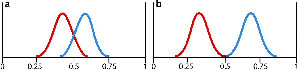
Figure 8. Distribution b shows greater polarization than a in terms of distinctness.
When there are more than two groups, some aggregation of all pair-wise comparisons must be made. Some care must also be taken in properly normalizing this measure when the number of groups differs across time or data sets. Both endogenous and exogenous measure versions can be extended unchanged to higher dimensions, but other measures (e.g., in terms of distribution density) may be appropriate as well. It is possible (and in some cases natural) to deploy and combine multiple measures of the same sense because they may each pick up different nuances.
What matters for polarization in this sense is how clearly distinct the groups are, regardless of the distance between them, their size, or their levels of internal cohesion. This seems to match what DiMaggio et al. call ‘bimodality’. People are polarized “insofar as people with different positions on an issue cluster into separate camps, with locations between the two modal positions sparsely occupied” (DiMaggio et al. Reference DiMaggio, Evans and Bryson1996, 694); distinctness focuses on the sparse intermodal region. Attitudes toward abortion between 1970 and 1990, for example, show clear and persistent distinctness (fig. 9).

Figure 9. Attitudes toward abortion, distribution by year, from the full sample General Social Survey 1977–94 (DiMaggio et al. Reference DiMaggio, Evans and Bryson1996).
2.7. Polarization Type 7: Group Divergence
While group distinctness captures how distinct the separation is between groups, regardless of how far away those groups are in their beliefs, group divergence captures the opposite: how distant the groups’ characteristic ideas are without attention to potential group overlap. This sense also fits the definition of ‘dispersion’ in DiMaggio et al. (Reference DiMaggio, Evans and Bryson1996), especially when combined with an assumption of bimodality. One simple measure for divergence will be the distance between group means, whether those groups are defined endogenously or exogenously. As figure 10 indicates, group divergence may increase while measures such as distinctness, spread, and coverage remain constant.

Figure 10. Attitude distribution b shows greater polarization than a in the sense of group divergence.
Like distinctness, the measure of divergence works unchanged for higher dimensions with appropriate distance measures, but some aggregation scheme must be chosen for more than two groups. If the groups are fully distinct, then one can also find the distance between the maximum value in one group to the minimum value in the next, that is, the width of the empty space between the groups. Both the distance between means and of extremes (and others) capture this sense of polarization, but they focus on different features of the distribution and thus can work complementarily, as long as researchers are careful to specify the measure used.
2.8. Polarization Type 8: Group Consensus
The beliefs of group members can be highly scattered across the spectrum or extremely focused on the group’s central ideology (fig. 11). The diversity of opinions within groups constitutes another sense in which those groups can be polarized, independent of how far apart their central ideas are and how distinct the groups are. Prima facie, the greater the variance in beliefs within groups, the more likely it would seem that members of one group might move toward common ground with other groups. The more single-minded or unanimous views are within the groups, the greater the polarization between them and the less likely any such conciliation.

Figure 11. Belief distribution b shows greater polarization than a in the sense of group consensus.
A simple and suggestive measure of groups consensus is the absolute deviation within each group, aggregated over all the groups (e.g., the size-weighted average). The smaller the variance within each distinct group, the greater this sense of polarization across the population. As previously mentioned, this is the main sense in which polarization has increased in the US legislature (McCarty et al. Reference McCarty, Poole and Rosenthal2008). It is not the case that the party lines have shifted much over the past few decades but rather that the party members have more consistently voted along the lines of their party.
If the position of the groups’ mean beliefs are fixed and close enough (low enough divergence), then a change that increases consensus also yields an increase in distinctness. But it is possible for the group consensus to change independently of any of the other measures. Depending on the measures used for each sense and the particular distribution being analyzed, consensus and distinctness may or may not be mathematically linked even though they are conceptually distinct.
2.9. Polarization Type 9: Size Parity
A society that has one dominant opinion group with a few small minority outliers seems less polarized than one with a few comparably sized competing groups. Groups are more polarized in this sense if the different clusters of beliefs are held by equal numbers of people (fig. 12). For example, a society in which a small group of 1% of the population with extremist views gains in popularity to capture a third of the population (while holding all the other measures fixed) is a society with increasing polarization.

Figure 12. Groups with comparable sizes are more polarized than a large group with smaller outliers; in the sense of size parity, belief distribution a is more polarized than b.
There are a few obvious measures for capturing size parity. If there are just two groups (which may not exhaust the population) then a direct subtraction of their sizes is perhaps sufficient. For larger numbers of groups it is preferable to consider measures that aggregate more intuitively. One example is the sum of the differences in size of each group from the mean group size. Using the proportions of the population for each group, one can also use an entropy measure or a diversity indicator such as the inverse Simpson index.
2.10. Further Considerations for the Senses of Polarization
The nine senses of ‘polarization’ outlined here offer only a starter set, and the senses can be multiplied quite quickly by a range of other factors.
2.10.1. Polarized versus Polarizing
As noted, ‘polarization’ can be used to label either the configuration of a population at a time or a particular dynamics in the change of a population configuration over time. It is said that American political opinion is currently polarized. That claim seems to involve one of the static measures discussed above. But ‘polarization’ may also be used to mark the process of becoming more polarized in one of these senses. In this second sense, a community may be marked by polarization as it is marked by increased spread, distinctness, or solidarity of the opposing groups, even if the static measure does not show polarization to any great extent on any of these scales. So, when we ask whether there is polarization in a society, one question that has to be asked is whether it is polarization in one of our static senses or polarization in one of the related process senses that is at issue.
2.10.2. Measure Independence and Combinations
Another kind of question that must be asked is whether multiple and perhaps mutually dependent clusters of measures are involved. The nine senses outlined are pair-wise independent: for any two senses one can construct an example of belief distributions showing that an increase in one sense can be accompanied by no change or even a decrease in the other. The concepts and their measures are not, however, completely orthogonal. Fixing the value of a third measure may force two others to be positively or negatively related, depending on the particular measures involved. Consider, for example, relations between spread, coverage, and dispersion while assuming a belief distribution that does not completely fill the space between 0 and 1. A simple measure for spread is the distance between the maximum and minimum observed value. Coverage is the proportion of bins in which at least one person holds that bin’s value. Dispersion is the average distance of data points to the population mean. To increase spread without varying coverage, we could move all the data points located at the upper extreme to larger-valued bins. To increase spread without varying dispersion, we can take occupants from near the upper edge and move one inward and another outward by the same distance. But if we fix the spread of the distribution, then moving points to increase coverage (by filling in intermediate bins) must change dispersion as well. Keeping coverage constant while increasing spread will likewise force an increase in dispersion.
Capturing senses of ‘polarization’ independently is vital for understanding the core conceptual elements of the social phenomena at issue. We think it is important to keep these different aspects of polarization distinct, particularly in those cases in which data may exhibit polarization in multiple senses. The most common measure of polarization in the political literature is probably bimodality, which is the idea that the population can be usefully broken down into two subpopulations. Polarization in this sense signals a balanced deviation from a moderate position. Fiorina and Abrams measure bimodality in American political opinion, for example, by tracing the drop in the percentage of respondents labeled moderate combined with balanced redistribution to both sides of the moderate position. They do not regard accumulation to only one side as a polarizing trend (Fiorina et al. Reference Fiorina, Abrams and Pope2005). But it is clear that a focus on bimodality alone merges and often blurs a number of the senses of ‘polarization’ outlined. Community fragmentation plays a role because bimodality demands exactly two distinguishable groups. The distinctness of those groups is also important; Fiorina and Abrams are invoking distinctness when they measure the drop in moderate view holders. Group divergence and spread are included because these increase when equal numbers of responses move to both sides, less so when they move disproportionately to one side. Neither group solidarity nor size parity is explicitly invoked in a concept of bimodality, although if there is too little solidarity or size parity then the two groups on each side of the issue may not be discernible as such. Importantly, however, many of the concepts commonly merged in bimodality may also vary independently.
2.10.3. Multiple Dimensions
As noted initially, we have focused on senses of ‘polarization’ that can obtain in one-dimensional distributions and for which appropriate measures can be formulated for a single-issue histogram. Other senses of the term, incorporating one or more of these, will be appropriate where more than one issue is at stake. One example of a sense of polarization requiring multiple dimensions is belief convergence. Given groups that are polarized on issue A, are these same groups polarized on B, C, and D? The more connected rival beliefs are within rival groups, the greater the polarization across the community. This can be measured using a data-clustering technique. Another example is belief coherence: are changes in one belief accompanied by analogous changes in another belief—a solidarity of ideas? Coherence of beliefs can be measured using correlations of the belief values across dimensions. Figure 13 illustrates beliefs on two axes showing the relative correlation of two opinions on two axes.

Figure 13. Beliefs on two topics, indicated on the axes, are correlated in b and not in a. Greater correlation of belief values across multiple issues marks greater polarization in the sense of belief coherence.
In measuring multiple opinions, all the senses of ‘polarization’ above will return with a new complexity. Groups may have tightly knit sets of opinions that are uniformly polarized in any of the senses noted. But, their opinions on different issues A, B, and C may turn out to be polarized in some of the importantly different ways we have tried to distinguish.
3. Modeling Polarization
Having disambiguated senses of ‘polarization’, we are now in a position to examine how various approaches to modeling basic mechanisms of polarization compare in terms of the specific types of polarization they are, and are not, able to produce. Where possible we indicate how each of the measures above changes as polarization as defined in the model increases. We cannot cover all models and model variations that have been offered; we concentrate on what we take to be the three central families of computational models that have been put forward, together with a model-suggestive theory from psychology. An evaluation of the various models that have been proposed, using the tools of our conceptual analysis, serves to clarify ways in which individual models can be seen as illuminating isolated facets of a much more complex social reality.
The first family of models that we consider targets cultural diffusion and differentiation as a basic mechanism for polarization. The extensive literature begins with Axelrod (Reference Axelrod1997) followed by significant further contributions in Klemm et al. (Reference Klemm, Eguiluz, Toral and Miguel2003a, Reference Klemm, Eguiluz, Toral and Miguel2003c, Reference Klemm, Eguiluz, Toral and Miguel2005), Flache and Macy (Reference Flache and Macy2006a), and Centola et al. (Reference Centola, Gonzalez-Avella, Eguiluz and Miguel2007). Bounded confidence and relative agreement models form a second family of models, in which the mechanism put forward for polarization is one in which updating on others’ opinions is constrained by a window or graded extent of prior agreement (Deffuant et al. Reference Deffuant, Amblard, Weisbuch and Faure2002; Hegselmann and Krause Reference Hegselmann and Krause2002; Deffuant Reference Deffuant2006). A third family we consider are models in the structural balance tradition (Heider Reference Heider1946; Cartwright and Harary Reference Cartwright and Harary1956; Harary Reference Harary1959; Macy et al. Reference Macy, Kitts, Flache and Benard2003; Klemm et al. Reference Klemm, Eguiluz, Toral and Miguel2005; Kitts Reference Kitts2006). Here the basic mechanism of polarization is a change in network links of amity and enmity, further developed in terms of opinion or belief and employing mechanisms of Hebbian learning and Hopfield networks. Beyond these three families of models, we also consider ‘group polarization’ from social psychology (Lord et al. Reference Lord, Ross and Lepper1979; Hogg et al. Reference Hogg, Turner and Davidson1990).
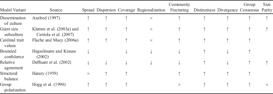
In the following sections, we consider each of these central families of models with an eye to the nine senses of polarization outlined above. The focus is on central mechanisms characteristic of each model family, the senses of polarization in which model output for each family falls, and the senses or aspects of polarization that fall outside the scope or beyond the reach of each model family. The goal is a comparative sketch of both promise and problems: the extent to which different approaches may offer explanatory mechanisms for phenomena that appear in some aspect of opinion dynamics but also the extent to which explanations offered may be incomplete or structurally limited by specific modeling constraints. Are there senses of ‘polarization’ that these models exhibit or capture particularly well? Are there senses of ‘polarization’ that will escape them? How good are these models in capturing plausible social psychological mechanisms of polarization, and in what sense? We offer a summary of the senses of ‘polarization’ connected with each model in table 1. In the sections that follow, we review in detail senses of ‘polarization’ and grouped patterns of phenomena in each of the model families.
Table 1. Senses Polarization Invoked, by Model
| Model Variant | Source | Spread | Dispersion | Coverage | Regionalization | Community Fracturing | Distinctness | Divergence | Group Consensus | Size Parity |
|---|---|---|---|---|---|---|---|---|---|---|
| Dissemination of culture | Axelrod (Reference Axelrod1997) | ↑ | ↑ | ↑ | × | ↑ | ↑ | ↑ | ↑ | ↑ |
| Giant size subculture | Klemm et al. (Reference Klemm, Eguiluz, Toral and Miguel2003a) and Centola et al. (Reference Centola, Gonzalez-Avella, Eguiluz and Miguel2007) | ↑ | ↑ | ↑ | × | ↑ | ↑ | ↑ | ↑ | ↑ |
| Cardinal trait values | Flache and Macy (Reference Flache and Macy2006a) | ↑ | ↑ | ↑ | × | ↑ | ↑ | ↑ | ↑ | |
| Bounded confidence | Hegselmann and Krause (Reference Hegselmann and Krause2002) | ↓ | ↓ | ↓ | ↓ | ↑ | ↓ | ↑ | ||
| Relative agreement | Deffuant et al. (Reference Deffuant, Amblard, Weisbuch and Faure2002) | ↓ | ↓ | ↓ | ↓ | ↓ | ↑ | ↓ | ↑ | ↑ |
| Structural balance | Harary (Reference Harary1959) | × | ↑ | ↑ | ↑ | ↑ | ↑ | ↑ | ||
| Group polarization | Hogg et al. (Reference Hogg, Turner and Davidson1990) | ↑ | ↑ | ↑ | × | ↑ | ↑ | ↑ | × |
Note. We mark how each sense varies with an increase in polarization as reported by the model description (↑ for a positive covariance and ↓ for a negative covariance) as well as other senses that covary because of mathematical constraints in connection with the explicitly identified senses (↑ or ↓) using measures appropriate for that model. We further mark those senses of polarization that cannot be affected by the models’ mechanisms (×) and leave blank those senses that may or may not be effected.
3.1. The Axelrod Tradition
Axelrod (Reference Axelrod1997) proposes that polarization can arise from an intuitive mechanism that would at first sight seem only to promote conformity and cultural convergence. We first review Axelrod’s original version of the model and discuss the senses of polarization it can and cannot produce. We provide the same treatment for three variants of the model that differ from the original in ways that affect polarization.
The basic premise is this: people tend to interact more with those like themselves and tend to become more like those with whom they interact. But if people come to share one another’s beliefs (or other cultural features) over time, why do we not observe complete cultural convergence? Axelrod acknowledges a number of proposed mechanisms for durable cultural differences—active social differentiation, preferences for extreme views, geographical isolation, specialization, and exogenous changes in the environment or technology—but his model relies on none of these. At the model’s core is a spatially instantiated imitative mechanism that produces cultural convergence within local groups but also progressive differentiation and cultural isolation from other groups. He refers to that differentiation as ‘polarization’.
Axelrod’s base model consists of 100 agents arranged on a 10 × 10 lattice such as that illustrated in figure 14. Each agent is connected to four others: top, bottom, left, and right. The exceptions are those at the edges or corners of the array, connected to only three and two neighbors, respectively.Footnote 3 Agents in the model have multiple cultural ‘features’, each of which carries one of multiple possible ‘traits’. One can think of the features as categorical variables and the traits as options or values within each category. For example, the first feature might represent culinary tradition, the second one the style of dress, the third music, and so on. In the base configuration an agent’s ‘culture’ is defined by five features (F = 5) each having one of 10 traits (q = 10): qf ∈ {0, 1, 2, 3, 4, 5, 6, 7, 8, 9}. For example, agent x might have a cultural signature specified by traits {8, 7, 2, 5, 4} while agent y has a cultural signature specified by traits {1, 4, 4, 8, 4}. Agents are fixed in their lattice location and hence their interaction partners. Agent interaction and imitation rates are determined by neighbor similarity, where similarity is measured as the percentage of feature positions that carry identical traits. With five features, if a pair of agents share exactly one such element they are 20% similar; if two elements match then they are 40% similar, and so forth. In the example above, agents x and y have a similarity of 20% because they share only one feature, their fifth: x 5 = y 5 = 4. For each iteration, the model picks at random an agent to be active and one of its neighbors. With probability equal to their cultural similarity, the two sites interact and the active agent changes one of its dissimilar elements to that of its neighbor. If agent i = {8, 7, 2, 5, 4} is chosen to be active and it is paired with its neighbor agent j = {8, 4, 9, 5, 1}, for example, the two will interact with a 40% probability because they have two elements in common. If the interaction does happen, agent i changes one of its mismatched elements to match that of j, becoming perhaps {8, 7, 2, 5, 1}. This change creates a similarity score of 60%, yielding an increased probability of future interaction between the two.

Figure 14. Typical initial set of “cultures” for a basic Axelrod-style model consisting of 100 agents on a 10 × 10 lattice with five features and 10 possible traits per agent. The marked sight shares two of five traits with the site above it, giving it a cultural similarity score of 40% (Axelrod Reference Axelrod1997).
In the course of approximately 80,000 iterations, the model process produces large areas in which cultures of traits on features are identical: the ‘local convergence’ of Axelrod’s title. It is also true, however, that arrays such as that illustrated do not typically move to full convergence. They instead tend to produce a small number of culturally isolated stable regions—groups of identical agents none of whom share features in common with adjacent groups and so cannot further interact. As an array develops, agents interact with increasing frequency with those with whom they become increasingly similar, interacting less frequently with the dissimilar agents. With only a mechanism of local convergence, small pockets of similar agents emerge that move toward their own homogeneity and away from that of other groups. With the parameters described above, Axelrod reports a median of three stable regions at equilibrium. It is this phenomenon of global separation that Axelrod refers to as ‘polarization’.
Which of the senses of polarization that we have outlined does Axelrod’s model capture? In his primary use of the term, Axelrod’s ‘polarization’ refers to stable, distinct, contiguous, and wholly culturally differentiated regions at equilibrium. An array is polarized in his sense when there are two or more stable regions, although we might also extend his usage by speaking of grids with a greater number of culturally distinct regions as being more polarized. In this way we can see Axelrod’s ‘polarization’ as a form of community fracturing even though measuring the number of groups in this model does not involve separating histograms at their basins of attraction as described above. Although the measure is different, the number of isolated regions in Axelrod’s model is clearly also a way to capture groups of agents with internally similar ‘beliefs’ separated from other groups with opposed beliefs.
A fundamental characteristic of Axelrod’s model is its multidimensionality: each feature represent a different dimension in which agents or groups can be the same or different. Although the categorical nature of the traits means that correlation cannot be applied, it is clear that the model exhibits polarization in the general sense of belief convergence described in section 2.11.3. In the equilibrium state, agents who have the same trait for the first feature will also have the same trait for the second, third, fourth, and fifth traits. That mix of traits will be (almost always)Footnote 4 completely distinct from the mix of traits of any other group; thus, data clustering will pick out the different groups cleanly.
Although the multidimensionality of Axelrod’s model fosters analysis through additional measures, the categorical nature of the traits precludes any notion of closeness and with it most of the measures of polarization we described above. One measure that does apply, expanded to higher dimensions, is coverage. By considering the three-dimensional histogram of agents’ cultures on the F × q discrete belief space, we can count the proportion of empty bins and watch the number grow as the population moves toward isolated homogeneous communities.
The result that different abutting communities cannot share any of their cultural traits also sounds much like distinctness, and the result that intragroup traits become homogeneous sounds much like group coherence, but these cannot be measured using histograms of beliefs. A notion of similarity in terms of the number of identical features and using measures based on Hamming distance or a similar alternative might be developed, however. For example, spread could be measured as the highest number of pair-wise dissimilar traits, and dispersion could be taken as average pair-wise dissimilarity. Both of these measures are greatest when there are isolated communities and zero when there is one homogeneous population. Extensions of this sort do seem to offer multidimensional categorical analogies to the senses of polarization outlined.Footnote 5 Thus, Axelrod’s model nicely instantiates some of the general concepts of polarization we have described, even though agents are not characterized in terms of opinions with cardinal belief values, and therefore other measures would be required to quantify most senses.
3.1.1. Expanding the Parameter Ranges
Axelrod notes a number of intriguing features of the model, many of which have been taken up in later work. Results turn out to be very sensitive to the number of features F and traits q used in the model. Altering numbers of features or traits changes the final number of stable regions but in opposite directions: the number of stable regions correlates negatively with the number of features F but positively with the number of traits q (Klemm et al. Reference Klemm, Eguiluz, Toral and Miguel2003b). In Axelrod’s base case with F = 5 and q = 10 on a 10 × 10 lattice, the result is a median of three stable regions. When q is increased from 10 to 15, the number of final regions increases from three to 20; increasing the number of traits increases the number of stable groups dramatically. If the number of features F is increased to 15, in contrast, the average number of stable regions drops to only 1.2 (Axelrod Reference Axelrod1997). Increasing the number of features decreases the number of stable groups. On reflection, the reason for this model sensitivity is clear. As the number of features F increases, agents have a greater probability of having something in common, increasing the probability that they will interact and thus increasing the probability that they will converge, resulting in fewer final stable groups. As the number of traits increases, however, it becomes less likely that agents will have matching traits on a given feature, diminishing the probability they will interact and thus increasing the probability of isolated groups. It turns out that achieving at least two stable groups at equilibrium is reliable only when the number of traits is greater than the number of features (Axelrod Reference Axelrod1997).
Axelrod also demonstrates that the results are sensitive to the size of the array. For an N × N lattice and q > F, the maximal number of stable cultural regions is reached when N = 15, falling monotonically with greater N. At N = 50, the number of stable regions is on average five, for example; at N = 100, the number falls to roughly two. Cultural diversity is increasingly difficult to achieve in larger populations, where total convergence is the typical result (Axelrod Reference Axelrod1997).
In addition to the number of culturally distinct groups, the size of those groups can be taken as a mark of polarization. In a series of extensions of the Axelrod model, Klemm et al. (Reference Klemm, Eguiluz, Toral and Miguel2003a, Reference Klemm, Eguiluz, Toral and Miguel2003b, Reference Klemm, Eguiluz, Toral and Miguel2003c, Reference Klemm, Eguiluz, Toral and Miguel2005) devise a measure for representing the degree to which a population is dominated by one homogeneous culture: the ratio of the largest stable region to the whole. If we let P = N × N be the size of the total population and P 1, P 2, … be the sizes of the subpopulations ranked by size, then their measure is P 1/P. When this “giant size ratio” equals 1 (i.e., when P 1 = P), there is just a single monoculture. As P 1/P moves toward 1/P, either the nondominant groups are getting larger or more groups are forming. One can interpret this measure as a rough alternative to the size parity measures presented in section 2.9.
Klemm et al. find that there is a specific value of the number of traits q* at which the giant size ratio changes from values near 1 to values near 0. For example, a 100 × 100 lattice with 10 features has a giant size ratio of nearly 1 as long as there are fewer than 55 traits. With more than 55 traits, the giant size ratio rapidly decreases: it only achieves values less than 0.1 when there are 60 traits, whereas below 54 traits the result is usually a single uniform group. For a given N and F, it is only within a very narrow band around q* that the giant size ratio takes on intermediate values.
Centola et al. (Reference Centola, Gonzalez-Avella, Eguiluz and Miguel2007) offer a further extension with a variation on Axelrod’s static array. In the Axelrod model, it is possible for two neighboring agents to become incapable of interaction, because their traits differ on all features, but later to regain that possibility through indirect alignment of features. As Axelrod notes, borders need not be permanent because contact with others may give an agent new traits that then allow interaction with a site it previously had nothing in common with. In the Centola model, in contrast, agents lose their common edge forever—like a broken link in a network—whenever they cease to share features in common. In this variation Centola et al. show that the specific point for the Klemm threshold q* increases by an order of magnitude, but the rapid transition from a single large group to many small ones remains.
Although the original model produces polarization in multiple senses (assuming analogous categorical measures), Axelrod uses only the sense we call community fracturing to define polarization, measured by the number of isolated culture groups. In the Klemm and Centola extensions, the authors focus on another of our senses of polarization: size parity. As outlined in section 2.9, polarization in the sense of size parity is maximized when all the groups have equal sizes and is minimized when there is one dominant group and the others are significantly smaller. Given the particulars of Axelrod’s base model, minimal size parity aligns exactly with a value of 1 for Klemm’s ‘giant size ratio’. For other values of Klemm’s measure, the fit is underdetermined. Klemm’s is a measure merely of the ratio of the largest group over the whole population. A Klemm measure of 0.5 will therefore occur in both of these cases: (1) two groups each with 50% of the territory and (2) one group at 50% and 100 others at 0.5%. Case 1 would be highly polarized by our measure of size parity, but case 2 would not register as polarized in this sense.
Although the ‘giant size ratio’ measure is easy to calculate and track, and although it does capture something important about the dynamics of this particular class of models, it fails to distinguish between these two very different cases. What is of more interest for us here is the shift in focus of what counts as polarization as one moves from Axelrod to later extensions. Although everybody involved is interested in exploring ‘polarization’, they are not analyzing the same social patterns. Klemm’s measure cannot distinguish between cases 1 and 2 above, Axelrod’s community fracturing sense would report case 2 as being much more polarized, and size parity would report case 1 as being more polarized. Because different senses can move independently and sometimes in opposite directions, this is a clear case in which it is not enough to just say that polarization is increasing without specifying the sense or senses of ‘polarization’ at issue.
Models in the Axelrod family continue to be studied because they are elegant and noteworthy for both their emphasis on multiple dimensions and the general result that endogenous rules favoring convergence can nevertheless drive a population to polarization (in certain senses). It turns out that a variety of senses of polarization, or their analogues, that are evident in the Axelrod family—dispersion, coverage, community fracturing, opinion cohesion, group divergence, group consensus, and size disparity—are typically not captured by other traditions. For each of these measures, however, an appropriate categorical measure must be used instead of the more familiar cardinal-valued representations in terms of belief or opinion. One may naturally wonder whether this style of model continues to produce such a variety of senses of polarization when the traits are considered to be values on a spectrum.
3.1.2. Cardinal-Valued Traits
As indicated by our use of histograms in explicating the senses of polarization above, much of the literature on belief polarization uses ordinal or cardinal-valued belief spectra, such as those derived from Likert scale surveys and discretized population data. Although still discrete, variables of this type come with a lesser-to-greater order and usually an implicit/assumed scale such that a value of 1 is closer to 2 than it is to a value of 5. This creates a metric space that allows the use of distance measurements between values. Making this move for the Axelrod model, the similarity of two agents can be calculated as how far apart their trait values are rather than just how many features have strictly identical traits.
Flache and Macy (Reference Flache and Macy2006a) explore this cardinal-valued variation with a model that allows some features to be categorical (nominal) and others to be ordered (metric). Categorical features are given distance 0 if identical and 1 otherwise. For the ordered features, the distance is simply the normalized absolute value of the difference in the trait values. Summing and normalizing by the number of features produces a pair-wise similarity score between zero and one. The probability of an interaction increases with the pair-wise similarity scores—as long as the similarity is above a threshold—in such a way that it is equivalent to Axelrod’s interaction rule with certain parameters. This model re-creates the cultural diversity results of Axelrod with similar parameters and also replicates a result of Klemm in which diversity disappears with even tiny levels of mutation.
Flache and Macy’s model produces less polarization when metric states are used instead of categorical ones, with the obvious explanation that there are more opportunities for being similar (even if just partially) to neighbors. Despite the change in mechanism and results, however, the basic model invokes the same meanings and measures of polarization as Axelrod’s original.
Flache and May further expand the model by adding a “bounded confidence” aspect to the basic mechanism. As we will see in section 3.2, Deffuant et al. (Reference Deffuant, Amblard, Weisbuch and Faure2002) and Hegselmann and Krause (Reference Hegselmann and Krause2002) propose a mechanism that has proven seminal in polarization modeling research. In a similar spirit, Flache and Macy restrict the ‘vision’ of their agents such that they are only influenced by agents within their sights. Combined with the Axelrod mechanism, effects turn out to depend strongly on the value of that vision parameter. If the range of vision is too low, then everybody ends up in his or her own personal culture; if the range of vision is too high, then the result is again a monoculture. For intermediate values of the vision parameter there is a smooth transition from one extreme to the other. The more variables that are cardinal valued rather than categorical, the greater the threshold must be in order to transition from maximal to minimal diversity equilibria. For each cardinal-valued feature, the added mechanism of vision generates groups of clustered trait values along that dimension; combined with the Axelrod mechanism this translates to less similarity of neighbors and hence more isolation—‘polarization’ in the sense of the number of culturally isolated groups at equilibrium. We could expect the specific values for other measures, such as group divergence and distinctness, to be effected by this added mechanism. A study along these lines would benefit from including these additional measures and comparing the levels of polarization across multiple senses.
3.1.3. Evaluating the Axelrod Tradition
The Axelrod family of models succeeds in producing a variety of senses of polarization, or their analogues, from a simple mechanism of similarity-based imitation across local interaction. It has a deep appeal because of this variety and the intuitive representation of cultures and interaction. But it should be noted that the Axelrod tradition also faces major limitations even within some of the areas to which it most clearly applies. In reality, social polarization of all sorts seems easy to produce, is robust across a wide range of characteristics, and often proliferates despite efforts to generate consensus. It is therefore natural to compare how changes in polarization in the model align with the social polarization we would expect.
In the Axelrod models, polarization only occurs strongly when the number of traits is greater than the number of features: the characteristics in which cultures can vary are few relative to the number of ways each characteristic can be expressed. It is not clear how we could systematically or objectively enumerate the number of either features or traits for real societies in order to check the plausibility of this claim. As a formal requirement for at least some cases, however, it may not be implausible. For example, one interpretation is that there must be more potential positions to take on each political issue than there are distinct issues on the table.
One of the results of Axelrod’s model is that polarization in the sense of culturally isolated groups is increasingly difficult to produce with larger populations, such that it is rare with grids larger than 50 × 50. This has the unintuitive interpretation that if you increase initial cultural trait coverage then you decrease the eventual trait coverage: starting off less polarized by that measure paradoxically eventually makes society more polarized by that and other measures. The same is true for spread, dispersion, and other senses of polarization. Although counterintuitive because more people seems to imply more space for isolated niches to form, the result is not inexplicable considering the mechanism at work. Greater initial diversity often registers as greater polarization in the nongroup senses, but it also means a reduced chance of agents being culturally isolated from their immediate neighbors or neighbors two, three, or four steps away. With enough people, everyone has some common ground with somebody else nearby, and that common ground facilitates imitation, and that imitation leads eventually to monoculture.
We have noted the methodological criticism that very different cases are assigned the same Klemm measure. In practice the common model outcome that results in a lower Klemm ratio is one in which there are more small groups each of which is only slightly larger. Instead of thinking of Klemm’s ‘giant size ratio’ as a measure of polarization, it might be better to think of it as a measure of cultural domination in which domination is decreased with either more groups or larger satellite groups.
The common reality of familiar forms of social polarization is that of roughly balanced oppositional groups. Polarization of the type that appears in the Axelrod models at equilibrium, in contrast, almost always either a is radically one-sided or b appears as a myriad of tiny groups. There is only a small window around the threshold q* in which a moderate number of moderately sized groups can be achieved as a final outcome, and even that is not robust to noise or the use of cardinal-valued features. Thus, the familiar social reality of group size parity polarization—a small number of equally balanced groups—is not something produced by either Axelrod’s mechanism or its extensions. We also note that the social world, along with almost all of its socially polarized subsystems, is not in equilibrium. The end-state polarized equilibrium of these models therefore cannot be expected to resemble the time series of opinions captured in sociological or political surveys.
A major appeal of the Axelrod model remains, despite the limitations noted. That such a mechanism alone can produce divergence does accord with some recent empirical research that indicates that in-group members can be drawn together without any demonstrable psychological out-group repulsion (Bicchieri Reference Bicchieri2006; Dreu et al. Reference De Dreu, Greer, Handgraaf, Shalvi, Van Kleef, Baas, Ten Velden, Dijk and Feith2010, Reference De Dreu, Greer, Van Kleef, Shalvi and Handgraaf2011). There are other classic results, however, that show that even neutral evidence on an issue can have a distancing effect on groups that are already separated (Lord et al. Reference Lord, Ross and Lepper1979). The basic mechanism of the Axelrod model, then, may be an important, albeit incomplete, piece of the polarization puzzle.
The point of a simple formal model is not to match the empirical dynamics precisely, of course, but to provide general insights into plausible mechanisms underlying the observed data. By seeing polarization broken down into its many senses it becomes possible to evaluate which of the many senses of polarization a model generates, and to what degree, as the model dynamics unfold. As noted earlier, Axelrod himself put forward several alternative mechanisms and formulations for social polarization. His aim is merely to show that a simple mechanism is sufficient to generate some of the stylized facts of polarization. It is meant to be insightful for one process, fully acknowledging the simultaneous operation of other mechanisms that can push and pull in different ways in different contexts. One such mechanism, already mentioned in passing, forms the core of the ‘bounded confidence’ family of models.
3.2. Bounded Confidence Family Models
In an influential series of articles, Hegselmann and Krause develop a ‘bounded confidence’ model of opinion polarization that functions in terms of mutual influence among those within a specific threshold of similarity (Hegselmann and Krause Reference Hegselmann and Krause2002, Reference Hegselmann and Krause2005, Reference Hegselmann and Krause2006). The primary results of the model are the formation of consensus given certain thresholds for who counts as ‘close enough’ and the formation of polarized groups with narrower thresholds. Furthermore, the number and location of the formation of polarized groups occurs at different points for different thresholds. Stated simply, this is another case of seeming incongruity between a plausible mechanism that can only increase the similarity of agents yet results in social fragmentation into separate ‘polarized’ attitude groups.
Opinions in the Hegselmann-Krause model are mapped onto the [0, 1] interval, with initial opinions spread uniformly at random. Belief updating is done by taking a weighted average of the opinions that are ‘close enough’ to an agent’s own. As agents’ beliefs change, a different set of agents or a different set of values can be expected to influence further updating. One way to think about the Hegselmann-Krause model is that all agents are effectively linked in a complete network, since it is possible for any agent to be influenced by any other. The primary mechanism of the model is then the threshold for what counts as ‘close enough’ for actual influence. Alternatively, one can think of the model as representing a dynamic network in which only those with opinions ‘close enough’ to an agent’s are linked in ways effective for belief updating.
Figure 15 shows the changes in agent opinions over time in single runs with thresholds ε set at 0.01, 0.15, and 0.25 respectively. With a threshold of 0.01, individuals remain isolated in a large number of small local groups. With a threshold of 0.15, the agents form two permanent groups. With a threshold of 0.25, the groups fuse into a single consensus opinion. These are typical representative cases, and runs vary slightly. As might be expected, all results depend on both (a) the number of individual agents and (b) their initial random locations across the opinion space. Given any threshold and sufficient individuals distributed evenly enough, the result of averaging will be inevitable consensus.
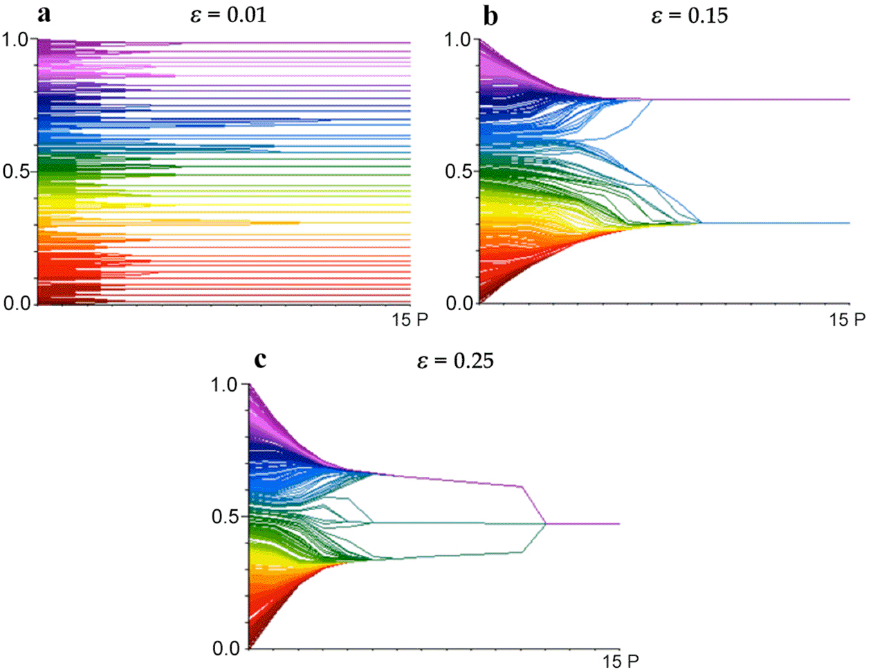
Figure 15. Example changes in opinion across time from single runs with different threshold values ε ∈ {0.01, 0.15, 0.25} in the Hegselmann and Krause (Reference Hegselmann and Krause2002) model.
An illustration of average outcomes for different threshold values appears as figure 16. What is represented here is not change over time but rather the final opinion positions given different threshold values. As the threshold value climbs from 0 to roughly 0.20, there is an increasing number of results with concentrations of agents at the outer edges of the distribution, which themselves are moving inward. Between 0.22 and 0.26 there is a quick transition from results with two final groups to results with a single final group. For values still higher, the two sides are sufficiently within reach that they coalesce on a central consensus, although the exact location of that final monolithic group changes from run to run creating the fat central spike shown.

Figure 16. Frequency of equilibrium opinion positions for different threshold values in the Hegselmann and Krause model scaled to [0, 100] (as original with axes relabeled; Hegselmann and Krause Reference Hegselmann and Krause2002). Slicing along each threshold value produces a histogram from average outcomes of the type used in defining the measures in section 2.
Hegselmann and Krause describe the progression of outcomes with an increasing threshold as going through three phases: “As the homogeneous and symmetric confidence interval increases we transit from phase to phase. More exactly, we step from fragmentation (plurality) over polarisation (polarity) to consensus (conformity)” (2012, 11). Here the term ‘polarization’ is being used to mean bimodality, already mentioned as a common and problematic identification in the literature. There are (at least) two ways to analyze the dynamics of the Hegselmann-Krause mechanism through our various senses of polarization: (1) how a population’s opinions shift as a run progresses (fig. 15) and (2) how the average distribution changes as the threshold increases (fig. 16).
The dynamics of an individual run make a few features immediately clear. First, in this model the groups are defined endogenously in exactly the way described in section 2.4. As a run progresses, the number of groups, and hence polarization in the sense of community fragmentation, decreases. Second, the averaging mechanism forces all the opinions within a group to be eventually identical. Polarization as group consensus therefore necessarily increases through the process. Third, because the opinion-averaging mechanism fuses any groups that are within the threshold of each other, the resulting groups are always completely distinct at equilibrium, another sense in which the mechanism necessarily increases polarization. In addition to these, it is clear from the second two frames of figure 15 that spread decreases as agents at extreme positions are pulled toward the population center, coverage decreases as agents coalesce into single-opinion groups, and the number of empty regions (regionalization) decreases along with the number of groups.
In Hegselmann and Krause’s own description of the results of increasing the threshold, it is clear that the dominant focus is on the number of groups, going from many to two and then to just one as the threshold increases. Although they emphasize the fact that at medium threshold values the population becomes bimodal, we take it that in the sense of community fracturing the polarization steadily decreases with increasing threshold values. The senses that change with increasing thresholds exactly mirror those that the mechanism generates in a single run—increasing the threshold serves to amplify the effects of that mechanism.
The Hegselmann-Krause model gives us the curious result that it is only in the senses of group distinctness and group consensus that polarization increases through model runs. In the population-based measures as well as community fracturing and group divergence polarization decreases. This is a very different polarization profile than the Axelrod family of models, in which most of the senses were shown to increase together. Even though the Hegselmann-Krause model produces distributions that many intuitively recognize as being highly polarized, they are polarized in only a couple of our senses. The opposite is true in many more. We are not proposing that these senses can be directly aggregated into some single measure. The full profile of all the senses is necessary to understand model dynamics both here and elsewhere.
The basic Hegselmann-Krause model, as outlined above, involves thresholds applied symmetrically; agents with opinions either to the left or right within a certain threshold are included in updating an agent’s opinion. Hegselmann and Krause also consider variations in which thresholds are applied asymmetrically, that is, with a different ‘inclusion’ to the left or the right, either (a) with the same bias for all agents or (b) with a bias keyed to the current opinion. The idea in the latter case is that those to the right pay more attention to those to their right; those to the left, more attention to their left. The former, not surprisingly, pushes the distribution patterns to one side, while the latter accentuates bimodality.
Because of boundary effects, applying the same bias to everybody brings size parity back into the picture: it is not just the locations of final groups that change but the sizes of those groups. Although this is still not a sense of polarization that Hegselmann and Krause invoke in describing the model, such an effect could be important in analyzing the application of these mechanistic variations to real social phenomena. Just as the first variant a above increases size parity, the second variant b increases the spread, dispersion, and divergence senses of polarization. All still decrease as the model runs over time, but they decrease less than in the base model. Hegselmann and Krause do provide intuitive explanations of the central mechanism and its effects, but incorporating specific measures of polarization for each sense would offer a precise mathematical and conceptual description of how the distribution of opinions changes.
Deffuant’s Relative Agreement Model.—Deffuant and his collaborators introduce a number of additional mechanisms in what they term a ‘relative agreement’ model. Whereas the bounded confidence mechanism updates agents’ opinions in terms of the average opinion of those within a certain threshold range of current opinion, Deffuant et al. update agents in randomized pair-wise interactions. Any agent may be paired with any other agent to determine influence, reflecting something like a completely connected underlying interaction network (Deffuant et al. Reference Deffuant, Amblard, Weisbuch and Faure2002; Deffuant Reference Deffuant2006; Meadows and Cliff Reference Meadows and Cliff2012).
More significantly, perhaps, the Deffuant model also replaces the sharp cutoff of influence in Hegselmann-Krause with continuous influence values. Agents are again assigned both opinion values and threshold (“uncertainty”) ranges, but the extent to which the opinion of agent i is influential on agent j is proportional to the ratio of the overlap of their ranges (opinion plus or minus threshold) over i’s range. The closer i and j’s opinions, the greater the overlap of their threshold ranges and the greater their influence on each other. The farther apart their opinions, as long as there is any overlap at all, the smaller the overlap and the smaller their influence. Deffuant et al. update both opinion centers and threshold ranges accordingly, resulting in the possibility of individuals with narrower and wider ranges. Given the updating algorithm, influence may be asymmetric: individuals with a narrower range of tolerance, which Deffuant et al. interpret as higher confidence or lower uncertainty, will be more influential on individuals with a wider range than vice versa.
For initial opinion values that are uniformly random on the [−1, 1] opinion space and initially identical threshold ranges, the results are very much the same as those of Hegselmann and Krause. Figure 17 shows a typical time progression of agents’ opinion dynamics, very similar in outcome despite the important differences in the treatment of thresholds.

Figure 17. Opinion dynamics in a population of 200 agents for an initial uniform threshold of 0.4, with the x-axis indicating the average number of iterations per agent (a proxy for time). Although the relative agreement mechanism differs from the bounded confidence mechanism, with the base parameters the opinion dynamics are very similar. From Deffuant et al. (Reference Deffuant, Amblard, Weisbuch and Faure2002).
One of the major goals of the Deffuant model is the attempt to produce extremism: convergence of opinion at an extreme end of the opinion range. Deffuant et al. note that this is possible in the Hegselmann-Krause model with asymmetric tolerance ranges but that it requires extreme parameters to produce. Related to this, the model is intended to demonstrate that a position that is initially extreme and held by only a few individuals can persuade the whole population to accept concordant extreme opinions. Deffuant et al. are able to produce the effect using ‘stubborn’ or ‘high-confidence’ individuals with narrow uncertainty thresholds placed at both ends of the opinion spectrum.
Although Deffuant et al. thoroughly explore the parameter space and reveal a variety of opinion dynamics in different value ranges, the result in figure 18 is the one most closely associated with ‘polarization’ phenomena and marks the primary departure from the Hegselmann-Krause model. Within this parameter zone the result is always two groups, one at each extreme, because the initially extreme agents at one end will never move to the other end. It is common for one-sided extremism to result even when there are the same number of initial extremists at both ends as in figure 18. Whether the result is most of the agents at one end or a split to both sides depends mainly on the random order of the pair-wise comparison updating.

Figure 18. When high-confidence (low-uncertainty, narrow threshold) agents are used at the ends of the spectrum, more than 98% of the initially moderate (green) agents are pulled to one side (in this case toward 1). Color indicates increasing confidence (lower ability to influence) as the population becomes more extreme and more homogeneous. From Deffuant et al. (Reference Deffuant, Amblard, Weisbuch and Faure2002).
Although the mechanism does not strictly force a large disparity in sizes, and in some runs the population is split nearly in the center, the typical result is a stochastic symmetry breaking such that most of the moderate central population snowballs to one side. Size parity is therefore a sense of polarization captured by the Deffuant et al. mechanism, more interesting precisely because it usually happens but is not obvious from the description of the agent update rules. The authors themselves admit that they did not foresee such a result.
Like the Hegselmann-Krause model, groups here must be defined endogenously by the opinion space. The number of groups, and hence polarization in the sense of community fracturing, decreases through time. Because of the stubbornness of the extreme agents, spread decreases only slightly because of a centrist pull. Coverage, regionalization, group distinctness, and group consensus change similarly as in the Hegselmann-Krause model, with some increasing and some decreasing.
Population dispersion decreases noticeably here as a by-product of the group size disparity. These two are the only senses of polarization that differ between the bounded confidence mechanism and the relative agreement mechanism. Polarization decreases in the sense of population dispersion, but the literature is rather quiet on that point. The most often-cited result is that polarization increases in the sense of size parity, together with group consensus and distinctness. There is something intuitive about bimodal movement of opinions away from each other on a spectrum. Here however the result is one of near uniformity at biased extremes. Deffuant’s intuitions regarding the influence of strongly held minority opinions shaping the population’s ideology are plausible ones but may not be the same phenomenon at issue in opinion polarization on abortion or gun rights, for example. Although the influence mechanism and the resulting opinion dynamics do seem to capture an important social force, it is not clear that ‘polarization’ is the most appropriate way to understand it.
3.3. Evaluating the Bounded Confidence Family of Models
Perhaps the greatest strike against this second family of models is that the central mechanism itself seems distinctly unreal. The main driver of the Hegselmann and Krause results is a mechanism of ‘peeling back from the edges’. The opinion distribution exhibited occurs for the very specific reason that agents at the left and right edges of the opinion space have no one to pull them left or right. They therefore drift toward the center, with either central or separated points of convergence dictated by the ε threshold. Despite the change in treatment of thresholds, the Deffuant et al. models inherit that central mechanism.
All models in this family cite and draw on a long tradition of belief averaging as a simple representation of the important psychological phenomenon of peer influence (French Reference French1956; DeGroot Reference DeGroot1974). But we are aware of virtually no evidence that real polarization occurs ‘from the edges’ as it does in these models or that it crystallizes in virtue of a specific distance from the edges as it does here. Indeed, there is a great body of evidence that the dynamics of developing polarization are quite different. The classic study by Lord et al. (Reference Lord, Ross and Lepper1979) shows groups in laboratory conditions that progressively polarize, increasing the distance between them over time despite balanced bodies of evidence (see also Miller et al. Reference Miller, McHoskey, Bane and Dowd1993; Kuhn and Lao Reference Kuhn and Lao1996). Cooper, Kelly, and Weaver claim that “one of the most robust findings in social psychology is that of attitude polarization following discussion with like-minded others” (Reference Cooper, Kelly, Weaver, Hogg and Tindale2001, 267).
Recall figure 9, showing American attitudes toward abortion between 1977 and 1993. That same figure serves to indicate the real limitations of the family of models considered. The models at issue can neither produce nor preserve the pattern of polarization evident there, that with a smaller central consensus with a heavy and consistent large group at the liberal end. Most noticeably, and in contrast to the reality of polarization, that liberal consensus would inevitably move right in models with a Hegselmann-Krause mechanism, and the large group of moderates would inevitable move to one side or the other using the Deffuant mechanism. Furthermore, such a phenomenon in the Deffuant models requires a careful planting of extremists with manually altered uncertainty thresholds to counteract the Hegselmann-Krause effect. Repeated studies show average attitudes among groups shifting toward extremes in terms of some mechanism not captured in the family of attraction-driven models considered here. The reality of increasing polarization of these familiar types, wherever it occurs, is a dynamic that this family of models is incapable of producing. These models also seem to capture an important and intuitive piece of the story of social opinion dynamics; however, it is not the whole story, and in many particulars it may not be most profitably read as a story of ‘polarization’ at all.
3.4. Structural Balance
Although less heralded in the computational literature, a third family of models for polarization has equal claim to consideration. Structural balance theory, also known as social balance theory, originated in the mid-1940s through the work of Fritz Heider, who studied patterns of belief coherence in individual psychology (Heider Reference Heider1946). In the mid-1950s, Cartwright and Harary generalized and formalized Heider’s theory using basic graph theory (Cartwright and Harary Reference Cartwright and Harary1956; Harary Reference Harary1959). Consider a set of nodes (e.g., people or countries) joined into a network capturing not just whether they have a relationship but also the valence of that relationship. In the base version, if two nodes are joined then they are either friends or enemies; later versions allow valence weights between −1 and 1 (Kulakowski, Gawronski, and Gronek Reference Kulakowski, Gawronski and Gronek2005). In the original analyses, a structure was considered ‘balanced’ whenever all paths—all unique sequences of links connecting each pair of nodes—had an odd number of negative links. Although there is some recent work that returns to the original ‘all paths’ version of balance calculations (Facchetti, Iacono, and Altafini Reference Facchetti, Iacono and Altafini2011), Abell (Reference Abell1968) made the case against longer paths being meaningful for social relationships, and in most structural balance research the fundamental unit of analysis has been a triad of three mutually linked nodes.
A triad is considered unstable if there is social pressure to change one of the relationship links; it is considered stable if there is no social pressure to change. The case of zero enmity is considered a stable triangle of friendship. A stable triad with two enmity links simultaneously captures the slogans ‘the enemy of my friend is my enemy’ and ‘the enemy of my enemy is my friend’. Those slogans also highlight the source of instability in the other possible patterns. If some agent A is friends with both B and C, but B and C are enemies, then A will be under pressure by both friends to choose sides, and B and C will be under pressure to make amends. In a triad with three mutual enemy relationships, there is pressure for two of them to ally against the third. Graphical relationships of these stable and unstable configurations are presented in the left portion of figure 19. Note that changing the valence of any single link in a stable triad will make it unstable, while changing the valence of any single link in an unstable triad will make it stable.

Figure 19. Left, four possible configurations of positive and negative links (ignoring rotation) as well as their classification under stable or unstable triads. Right, four larger structures capturing different types of stable and unstable social networks.
Larger social systems are classified as ‘balanced’ if all triads are stable, ‘unbalanced’ otherwise, with the level of instability typically calculated as the proportion of stable triads in the network as a whole. There are three types of stable configurations in larger networks: universal harmony, factions, and mixed networks, depicted on the right side of figure 19. In balanced networks with universal harmony, all links are friendship links. In factions, the network exhibits groups of mutually friendly nodes separated entirely from each other by enmity links. Mixed networks contain both positive and negative links in such a way that the network is balanced without forming factions.
It is easy to envisage a dynamic through which a network with initially randomly assigned valences can move toward a balanced network step by step. For example, (1) choose a triad at random; (2) if it is stable, do nothing; (3) if unstable, the valence of a random link in that triad is ‘flipped’ from positive to negative or vice versa. Flipping that valence may well make neighboring triads that also used that link unstable, of course, but as the process continues the network can be expected to move toward one of the balanced network configurations. In fact, given enough time any such random walk-like dynamic will eventually reach an equilibrium stable configuration.
A promise for understanding polarization can be seen in that dynamic. It is easy to prove that, for any complete network, progressively flipping valences within unstable triads will necessarily lead to either universal harmony or (with much higher probability) a ‘social mitosis’ resulting in precisely two groups, linked only by friendship internally and only by links of enmity between the two groups (Wang and Thorngate Reference Wang and Thorngate2003; Sack et al. Reference Sack, Flocken, Grim, Bramson and Berger2014). Social networks that are less than fully connected allow for more than two factions and the possibility of mixed networks, but the pattern toward social mitosis of the groups is still very much a dominant one (Hummon and Doreian Reference Hummon and Doreian2003).
In order to use structural balance as a model for opinion polarization, we must first interpret it in terms of opinions, beliefs, or attitudes rather than friends and enemies. The most direct way to achieve this is by assuming that agents hold beliefs on some topic. Agents who agree in their belief have a positive link, while those who disagree have a negative link. This interpretation makes both the stability and instability of triads as well as factional splitting natural: a network is balanced whenever all and only people who hold opposite beliefs disagree. The modeling implication for polarization is this: perhaps we see so much polarization because almost all stable opinion configurations within a population are polarized in this way. There is some empirical evidence for changes in social and political relations operating in roughly this way (Hart Reference Hart1974; Facchetti et al. Reference Facchetti, Iacono and Altafini2011; Kunegis Reference Kunegis2014).
What senses of polarization can a structural balance mechanism produce? As outlined, the basic dynamics are driven by increasing network ‘balance’, but on an interpretation in terms of agreement and disagreement there are implicit belief changes as well. We can assign all nodes of a stable triad with all positive ‘agreement’ links a belief of either p or ¬p. In a stable triad with two positive ‘agreement’ links and one negative ‘disagreement’ link, we can assign p to two nodes and ¬p to one, or ¬p to two and p to one. But there is no way to assign p and ¬p to nodes of unstable triads of agreement and disagreement without some node being assigned both p and ¬p. The basic mechanism of structural balance proceeds by changing link valences, and this is equivalent to changing beliefs so that the relationships of agreement and disagreement change appropriately.
Here we might suggest a model in which agents may have beliefs 1 or −1 but in which agents in ‘frustrated’ positions (i.e., nodes in unstable triangles) are assigned intermediate belief values that are the average across all neighbors of link valence × belief. If an agent’s only connection is a negative ‘disagreement’ link to a neighbor with belief =1, that agent will have a belief = −1, for example. If an agent has disagreement links to both a neighbor with belief = 1 and a neighbor with belief = −1, his belief will be 0 as the average. If a node has agreement links to two neighbors with beliefs = 1 and an agreement link to a neighbor with belief = −1, his intermediate belief value will be the link valence-weighted average of 1/3. As a final example, a node with an agreement link to a neighbor with belief = 1/3 and a disagreement link to a neighbor with belief = 2/3 will have an intermediate belief = −1/9.
Given this assignment of intermediate beliefs, we can suggest a dynamics for belief revision that uses the basic mechanisms of structural balance theory, although within a model of opinion change. Consider a randomly chosen node, and suppose that the product of link valence × neighbor values used to calculate the current belief of that node is positive—equivalently, whether its current value is positive. We then change the valence of random link, if any, that will result in a recalculation of belief value that moves that value further in the positive direction. If we randomly choose a node for which that product is negative—such that its current value is negative—we change the valence of a random link, if any, that will take its value further in the negative direction. Our conjecture is that a belief dynamics of this sort, appropriate to interpretation in terms of opinion polarization, will characteristically show a pattern of opinion mitosis toward belief extremes of 1 and −1 that parallels social mitosis in the original structural balance model.
What senses of polarization could such a model capture? What counts as ‘polarization’ under structural balance theory is clearly community fracturing, a move from something like the unstable mixed diagram to the stable factions diagram in figure 19. A network that is polarized in opinion through analogous mechanisms will also have factions in which all agents within each faction hold the same belief of either 1 or −1. Multiple groups of nodes holding the same belief can exist as long as there are no direct links between those same-belief factions. The degree of polarization in the sense of community fracturing can then be measured as the number of such groups.
Our conjecture is that final histograms of community-fractured (or factionalized) belief configurations will show beliefs close to 1 and −1; fully balanced systems will converge to the extremes, and only stable mixed configurations would show intermediate values in the final histograms. For these outcomes, the population-based senses of polarization—spread, dispersion, coverage, and regionalization—could not be usefully applied to compare final outcomes. Dispersion and coverage could be used, however, to track movements in population beliefs as the network stabilizes. Coverage would decrease as nodes with intermediate values push to extremes by mechanisms of triad balancing, with an increase in polarization in the sense of section 2.3. Polarization in the sense of the dispersion of beliefs increases as agents move to any stable configuration. Polarization as distinctness will increase along with coverage and dispersion as a population factionalizes, but it should be noted that none of these will necessarily progress monotonically; as in the original structural balance model, a change that increases the balance of a local triad may cause imbalance in other triads sharing one of its links. Size parity can also be measured as an opinion network evolves, but it is neither explicitly nor implicitly part of structural balance.
A fairly glaring limitation of models in the structural balance tradition should also be mentioned. As early as 1964, Abelson notes that computational models of opinion dynamics can easily fail by inevitably producing a radically unrealistic convergence of opinion to the center (Abelson Reference Abelson1964). Computational models that produce ‘polarization’ as inexorable drives to exclusive polar extremes of −1 and 1 will be radically unrealistic in the opposite direction. Structural balance models, whatever their other virtues, are clearly in this category.
3.5. Other Signed Networks
A number of other models produce results closely related to structural balance, using a Hopfield mechanism of dynamic attraction that also echoes aspects of similarity interaction in Axelrod (Macy et al. Reference Macy, Kitts, Flache and Benard2003; Flache and Macy Reference Flache and Macy2006b; Kitts Reference Kitts2006). In a Hopfield network, edge weights are determined through local calculations similar to those proposed in the section above but in which each node’s attribute is set to 1 or −1 depending on whether it is above or below 0 (Hopfield Reference Hopfield1982). In Macy et al. (Reference Macy, Kitts, Flache and Benard2003), nodes are characterized with either one or more binary states or one or more continuous states between 1 and 0. Link weights, or influence levels, are updated in Axelrod fashion as a function of the similarity between two linked nodes. If they occupy the same spot in the state space, the link between them becomes increasingly positive; if not, increasingly negative. Node characteristics are asynchronously updated by taking the link-weighted average node characteristics across one’s local neighbors and checking it against a threshold, then moving up to 1 or down to 0 accordingly. Where multiple characteristics are used, the process is repeated for each one independently.
The Macy model is not conceived in terms of structural balance among triads but rather in terms of the accord between a node’s values and those of its neighbors. Feature values for each node get pushed and pulled until every node’s features are minimally different from its network neighbors’ nodes. Just as in Axelrod, similarity-based influence is crucial, although similarity here is to all neighbors rather than pair-wise. Here, neighbors who are more different than average are pushed away to reinforce the difference. Despite these differences in conception, with binary agents the dynamics of the Macy model produce configurations precisely like those of structural balance. Here again the result is a ‘polarization’ in which factions of agents with similar characteristics are separated from those with other characteristics. If more features are used to characterize agents, it is possible for many more than two unique factions to persist at equilibrium. For each group, however, there must be some similarity with all other groups except one. For example, there could be stable groups of {0, 0}, {0, 1}, and {1, 1}, a multidimensional scenario invoking polarization as ‘belief convergence’ as outlined in section 2.10.3. Here, as in its structural balance predecessor, a homogeneous distribution is stable, but starting from a random assignment of characteristic values there is a vanishingly small probability of such a result. A sufficient exogenous shock, moreover, will knock the system out of a homogeneous situation and will usually lead again to a ‘polarized’ outcome. All of these are aspects of interest in the model. But because the results echo those of structural balance, the same senses of ‘polarization’, with the same limitations, will apply.
With a goal of generating dynamics indicative of social norms, Kitts (Reference Kitts2006) offers a further variation that incorporates intentional sanctioning behavior. Contagion-based influence is enhanced with frameworks for punishment and reward in terms of utility functions. Edge weights and therefore influence levels are updated using a Hebbian reinforcement learning algorithm. Here again, although not explicitly built into the model, the updating rule combined with the use of utility functions produces a result closely related to structural balance theory. Here and in other models (Flache and Macy Reference Flache and Macy2006b) results are again similar across a variety of parameter variations, with senses of polarization that are again those of the base structural balance model.
3.6. Group Polarization in Social Psychology
Up to now our focus has been on the three major families of computational models applied to phenomena of polarization. The term ‘polarization’ has also appeared in other literature without being operationalized into a formal model. Here we discuss one such case for which something approaching a model can be abstracted from the literature, at least close enough to be worthy of inclusion.
The experimental findings of Lord et al. (Reference Lord, Ross and Lepper1979) on belief polarization show that individuals tend to reinforce and move their beliefs in a more extreme direction when exposed to mixed evidence that, prima facie, would seem to lead to a more centrist position. Extending this finding further, self-categorization theory within social psychology defines ‘group polarization’ as the “conformity to a polarized norm which defines one’s own group in contrast to other groups within a specific social context” (Hogg et al. Reference Hogg, Turner and Davidson1990, 77). The theory predicts that in the context of confrontation with another group or other groups, in-group discussion will yield a “consensual group position that is more extreme than the mean of the individual group members’ prediscussion attitudes in the direction already favored by the group” (78). In the case of a centrist group confronted with groups on both sides, the prediction is a tighter focus on the mean. Although psychological explanations are provided for these attitude movements, they have not been operationalized as formal mechanisms.
Self-categorization theory posits that a group’s norm is actually further away from the population’s mean attitude than the members’ mean attitudes. When confrontation makes the issue salient, the group members adjust their attitudes to the perceived group norm and thus exaggerate their attitudes. This force bootstraps itself over time to produce increasingly extreme positions for members of the groups on the edges of the population. But the same mechanism pushes groups toward the population mean when confronted with groups more extreme than they are. Although the work in social psychology does not provide us models or opinion data, we can still refine our understanding of the claims being made by analyzing them in terms of our senses of polarization.
The theory is already conceived in terms of groups, so the appropriate senses of polarization will be the group-based ones. We can understand the claim that confrontation with an external group pushes the group mean to the perceived group norm as an increase in polarization in the sense of group consensus (decreased variance of in-group attitudes). The specific claim regarding the direction and amount of movement is relative to the external group(s) and thus can best be captured as an increase in divergence. This is also consistent with the case in which the focal group is sandwiched between extreme groups, increasing divergence by narrowing on to the mean value. There is no mention in the theory of a change in the number of groups, or of the focal group splitting, so community fracturing is not a sense relevant to this theory. Although the combined changes in group consensus and divergence are likely to produce an increase in distinctness, spread, dispersion, and coverage as well, there is nothing explicitly said about the dissimilarity of the groups beyond the direction and magnitude of their intragroup and intergroup differences. The ‘group polarization’ of self-categorization theory thus can be fully described in terms of consensus and divergence, although the dynamics of belief change may also show spread, dispersion, coverage, and distinctness.
4. Conclusion
With nine disambiguated senses and measures for ‘polarization’—spread, dispersion, coverage, regionalization, community fracturing, distinctness, divergence, group consensus, and size parity—we have attempted to evaluate the three major families of computational models that have been offered in the literature: the Axelrod family of cultural diffusion models, bounded confidence and relative agreement models, and structural balance models layered with belief transmission. To those we have added the prospect of models built with the fundamentals of self-categorization theory within social psychology.
An overview of results is shown in table 1. In the Axelrod tradition, ‘polarization’ in the sense put forward in the original (Axelrod Reference Axelrod1997) model and in the Flache and Macy (Reference Flache and Macy2006a) extension to cardinal traits is polarization in the sense of community fracturing. In the Axelrod-tradition models of Klemm et al. (Reference Klemm, Eguiluz, Toral and Miguel2003a, Reference Klemm, Eguiluz, Toral and Miguel2003b, Reference Klemm, Eguiluz, Toral and Miguel2003c, Reference Klemm, Eguiluz, Toral and Miguel2005) and Centola et al. (Reference Centola, Gonzalez-Avella, Eguiluz and Miguel2007), polarization as size parity is emphasized instead, with a similar link to other senses. We have found other senses of polarization, or plausible analogues, to be mathematically linked to the central phenomenon of community fracturing, increasing as it does. But none of these models is appropriate to polarization in the sense of regionalization. Although the senses of polarization presented here are logically independent and mathematically pair-wise independent, given the modeling constraints of the Axelrod family they become mathematically linked to each other. One implication is that models of this first family will prove inappropriate for any empirical case in which polarization occurs in some of the senses outlined but not in others.
Community fracturing is the sense of polarization that is the focus of the Axelrod family of models. But it is a decrease in community fracturing, together with an increase in group consensus, that is taken as the mark of polarization put forward in the bounded confidence model of Hegselmann and Krause (Reference Hegselmann and Krause2002). The same holds for the Deffuant et al. (Reference Deffuant, Amblard, Weisbuch and Faure2002) and Deffuant (Reference Deffuant2006) models, although in these models polarization as size parity appears as well. Here again other senses of polarization are mathematically linked, although often with a different direction than in the Axelrod models: it is decreases rather than increases in spread, coverage, and distinctness that accompany polarization in the sense at issue here. A different clustering of senses of polarization might well encourage profitable empirical investigation. The existence of social phenomena that exhibit one cluster of senses of polarization rather than another might support a hypothesis of one model mechanism rather than another. Our senses of polarization remain pair-wise logically independent, however, and here as before we have a family of models that will apply only to cases in which a particular cluster of senses inevitably occur together.
Extensions of the structural balance model offer a third family of computational models, in which polarization is put forward as community fracturing, divergence, and group consensus (Heider Reference Heider1946; Cartwright and Harary Reference Cartwright and Harary1956; Harary Reference Harary1959; Macy et al. Reference Macy, Kitts, Flache and Benard2003; Flache and Macy Reference Flache and Macy2006b; Kitts Reference Kitts2006). Mechanisms in some extensions incorporate aspects of the Axelrod model, and distinct senses of polarization are mathematically linked in ways similar to the Axelrod family. As noted, the structural balance family also has the downside of producing polarization only as migration to absolute opinion extremes on a spectrum. We have sketched the possibility of a more formal model using the mechanisms of group polarization in self-categorization theory (Lord et al. Reference Lord, Ross and Lepper1979; Hogg et al. Reference Hogg, Turner and Davidson1990), which exhibits divergence and group consensus but does not touch on polarization in the sense of community fracturing or size parity.
The first conclusion, we suggest, is that there is a need for attention to different senses of polarization in both the empirical and modeling literature. Different and apparently rival claims regarding whether America is becoming increasingly polarized, for example, may be addressing polarization in importantly different senses. We have shown that different families of computational models offered as mechanisms for opinion polarization produce very different phenomena, with very different connections, under that ambiguous term.
A second conclusion is that none of the families of available computational models is adequate to capture all of the senses of polarization described, particularly with an eye to producing polarization in those logically independent senses independently. If there are senses of polarization that do in fact always appear together, or do so within particular social phenomena, this potential shortcoming may be a hidden strength: in that case one or another of these model families may offer a plausible single mechanism behind clusters of polarization phenomena. Our suspicion, however, is that real phenomena of polarization are various enough, and subtle enough, that a full understanding will require a suite of models capable of something more: capable of producing polarization in all of its senses and with appropriate independence under appropriate circumstances. That is a modeling framework that does not yet exist. The current project highlights both the value of such a broadly capable framework and some of the specific targets within the literature of polarization that it would need to include.


