INTRODUCTION
Lymphatic filariasis (LF) is a tropical disease, which is caused by lymphatic-dwelling filarial parasites and is transmitted by mosquitoes that engorge the immature larval forms (microfilariae, mf) with a blood meal. Wuchereria bancrofti is responsible for >90% of all infections worldwide, while Brugia malayi and Brugia timori account for the remaining infections. Chronic infection with LF can cause gross swelling of extremities or the scrotum (lymphoedema, hydrocoele). The Global Programme to Eliminate Lymphatic Filariasis aims to eliminate this debilitating disease as a public health problem (World Health Organization, 2006). Yearly mass treatment is provided to reduce the mf reservoir to such low levels that transmission becomes insignificant and is eventually interrupted. However, questions are being raised about the feasibility of elimination (Gyapong and Twum-Danso, Reference Gyapong and Twum-Danso2006). In fact, we do not know how long mass drug administration should be continued, how that depends on local conditions, or how we can establish that transmission interruption is achieved. Models can help to answer these questions and further development of mathematical models has been identified as a priority in LF research (Dadzie, Basáñez and Richards, Reference Dadzie, Basáñez and Richards2004).
Several models have been developed for the simulation of LF transmission and control (Chan et al. Reference Chan, Srividya, Norman, Pani, Ramaiah, Vanamail, Michael, Das and Bundy1998; Plaisier et al. Reference Plaisier, Subramanian, Das, Souza, Lapa, Furtado, Van der Ploeg, Habbema and Van Oortmarssen1998; Rochet, Reference Rochet1990). All three models were quantified for W. bancrofti infection and validated using the detailed longitudinal epidemiological and entomological data that were available from urban Pondicherry in India (Chan et al. Reference Chan, Srividya, Norman, Pani, Ramaiah, Vanamail, Michael, Das and Bundy1998; Subramanian et al. Reference Subramanian, Stolk, Ramaiah, Plaisier, Krishnamoorthy, Van Oortmarssen, Amalraj, Habbema and Das2004). Thus far, the role of these models in decision support in control programmes is still modest. The main reason is that model predictions made for Pondicherry are not necessarily generalisable to other areas. If adjustments are made for differences in exposure to mosquito bites, then the model should be valid for other Indian areas, assuming that the basic biological assumptions are correct. However, the model cannot be used in regions with other vector or parasite species, because of known differences in the transmission dynamics (Southgate, 1992; Snow and Michael, Reference Snow and Michael2002; Snow et al. Reference Snow, Bockarie and Michael2006). To support decision making in the elimination programmes worldwide, we need vector-parasite specific, validated model variants (Dadzie et al. Reference Dadzie, Basáñez and Richards2004; Stolk, de Vlas and Habbema, Reference Stolk, de Vlas and Habbema2006).
The LYMFASIM program provides a flexible framework for simulating LF transmission and control (Plaisier et al. Reference Plaisier, Subramanian, Das, Souza, Lapa, Furtado, Van der Ploeg, Habbema and Van Oortmarssen1998). It can easily be adjusted to reflect the transmission dynamics in specific areas or to test models with alternative assumptions about the mechanisms involved in transmission. In this paper, we show how the parameters of LYMFASIM can be quantified to simulate W. bancrofti transmission by Anopheles mosquitoes in African communities. Emphasis is on capturing the general epidemiological patterns, but also the differences between communities. Therefore, the model is tested against cross-sectional data from many different locations, including data on the relationship between mosquito biting rates and local endemicity levels. A detailed sensitivity analysis is performed to explore how changes in parameter values influence the predicted long-term impact of mass treatment. For another example of the applicability of such an approach to modelling the transmission and control of another vector-borne infection, we refer to Smith et al. (Reference Smith, Maire, Ross, Penny, Chitnis, Schapira, Studer, Genton, Lengeler, Tediosi, De Savigny and Tanner2008, in this special issue).
MATERIALS AND METHODS
The LYMFASIM simulation model
LYMFASIM simulates the spread of W. bancrofti in a human community and the impact of control measures. A formal mathematical description of the model is provided elsewhere (Plaisier et al. Reference Plaisier, Subramanian, Das, Souza, Lapa, Furtado, Van der Ploeg, Habbema and Van Oortmarssen1998). Appendix 1 summarizes its main features and Table 1 explains the symbols that are used in the following section. A schematic representation of the variables and processes involved in transmission is provided in Fig. 1.
Table 1. LYMFASIM parameters with their nominal values for simulating transmission of lymphatic filariasis by Anopheles mosquitoes in African communities
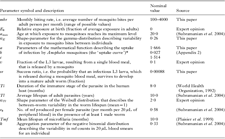
* L3=a(1−exp (−(bM)c). See Appendix 2 for further explanation.
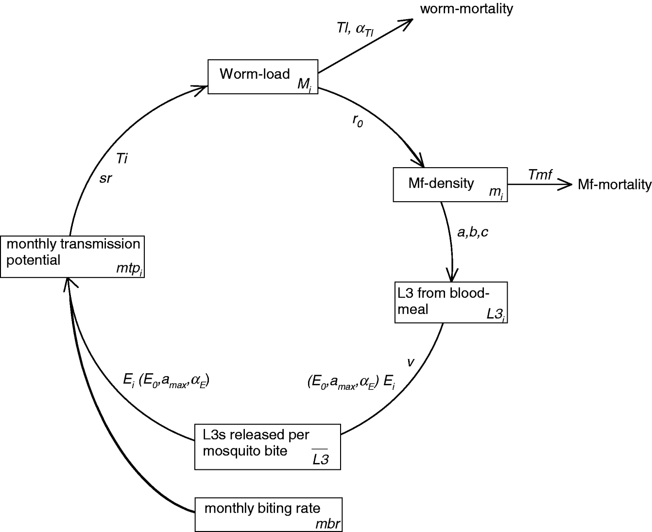
Fig. 1. Schematic representation of LYMFASIM, showing the processes that determine parasite transmission and the worm load in humans. The diagram shows the time-dependent model variables (boxes) and their interrelation (arrows). The associated model parameters are given along the arrows. Subscript ‘i’ indicates variables and parameters that vary between individuals. Processes related to optional immune responses are not included in the figure. See Appendix 1 for further explanation.
Quantification of the model for Africa
In a previous study, all parameters of LYMFASIM were quantified for simulating the transmission of Wuchereria bancrofti by Culex quinquefasciatus mosquitoes in Pondicherry, India (Subramanian et al. Reference Subramanian, Stolk, Ramaiah, Plaisier, Krishnamoorthy, Van Oortmarssen, Amalraj, Habbema and Das2004). We now set out to quantify the parameters for Africa. However, we changed the assumptions about immunity. The Pondicherry model included strong acquired immunity to explain that infection levels declined in elderly individuals (Subramanian et al. Reference Subramanian, Stolk, Ramaiah, Plaisier, Krishnamoorthy, Van Oortmarssen, Amalraj, Habbema and Das2004). Epidemiological data from Africa provide no indication of patterns consistent with such acquired immunity (Stolk et al. Reference Stolk, Ramaiah, Van Oortmarssen, Das, Habbema and De Vlas2004), and we discard it in the current model.
Some model parameters can take the same value in the models for Pondicherry and Africa because their value is independent of the area under study and vector species. This presumably applies to parameters that relate to infection in the human host, including several parameters of the parasite life cycle (Tl, Ti, Tmf, r 0, αTl) and the aggregation parameter (k) of the negative binomial distribution that quantifies the stochastic variability in mf counts in human blood samples. For the age-pattern in human exposure to mosquitoes, we assume that the exposure is zero in newborns (E 0) and that the maximum exposure is achieved in adults at age 20.
The uptake curve, which describes the relation between the mf density in human blood and the number of L3 developing in mosquitoes after a blood meal, depends on the vector species involved in transmission. The uptake curve was quantified for Anopheles by analyzing published data from feeding experiments (see Appendix 2). The estimated curve shows ‘facilitation’, which means that the number of L3 developing in mosquitoes from a blood meal increases initially at a rate higher than that expected from a linearly proportional relationship with the mf density in the human blood. Only at higher mf densities, limiting mechanisms seem to operate so that saturation occurs (‘limitation’).
The demographic parameters vary considerably between India and Africa, but within Africa they also vary between locations. For the current study, we take the overall population in Sub Saharan Africa as reference. We used the Revised Global Burden of Disease 2002 estimates of numbers of deaths by age and sex in the WHO ‘AFRO Region’ as a whole to calculate average age-specific death rates. (Data can be downloaded in spreadsheet format from the World Health Organization website, www.who.int.) These death rates were then used to construct a life table for the African region. Age-specific fertility rates for Sub-Sahara Africa were available from the US Census Bureau (2004). Exact quantification of fertility and mortality rates does not necessarily result in realistic age-structure of the simulated population, if historic trends in the rates over time and migration effects are ignored. To verify whether the age-structure of the simulate population is sufficiently adequate, we compared it with published population pyramids for sub Saharan Africa (US Census Bureau, 2004).
The average monthly biting rate (mbr) was the only parameter which we assumed to be varying between communities. We adjusted this parameter to simulate different endemicity levels. From published entomological studies, which measured the annual biting rate based on repeated all-night human landing catches, we estimated the range of possible values for the average mbr.
Two parameters were unknown and were estimated by fitting the model to data: (1) the success ratio sr, i.e. the probability that an infectious L3 larva, which is released during a mosquito blood meal, survives to develop into a mature adult worm; and (2) the variability in exposure to mosquito bites (defined by shape parameter αE of the gamma distribution). The Pondicherry-derived estimates for these parameters cannot be used because they were conditional on the inclusion of acquired immunity. In fact, a third parameter is also unknown, namely the fraction of the L3 larvae resulting from a single blood meal that is eventually released by a mosquito (v). However, v and sr are linear multiplication factors in the same sequence of calculations and cannot be estimated independently; therefore, we fixed v at a biologically plausible value of 0·1 and only estimated the success ratio sr.
Fitting procedure
We did a grid search to determine the values for the two unknown parameters that resulted in the best fit of model outcomes to data, based on visual assessment. For each pair of values for the success ratio (sr) and variability in exposure (αE), we performed a series of 3100 simulation runs. Each series consisted of 100 repeated runs for 31 different mbr values, ranging from 100 to 4000 bites per person per month (mbr 100, 150, …, 1000; larger increments thereafter). All runs started with a 125-year ‘burn-in’ period to achieve a dynamic equilibrium endemicity level and a population with stable age-sex composition and an average size of about 6000 individuals. The results of each series of runs were summarized, to allow comparison with field data.
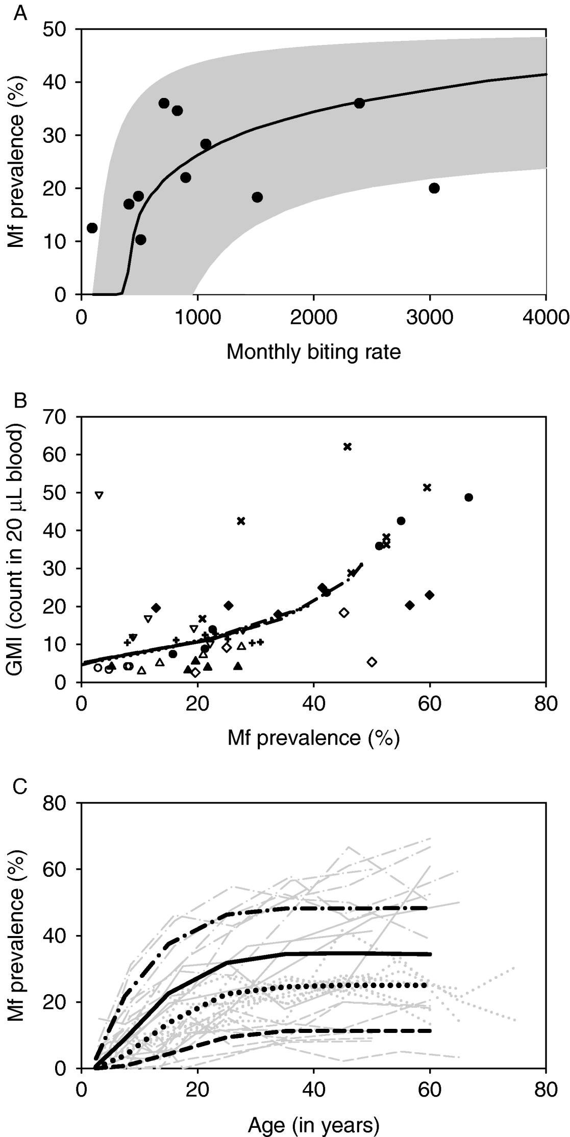
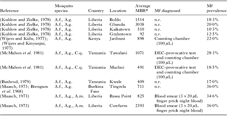
A well-fitting model had to satisfy the following three criteria. Firstly, the simulated relationship between mbr and overall mf prevalence should match that observed in various localities of the African region. Observed data about the relationship between overall mf prevalence and average monthly biting rate were obtained from a PubMed literature search. We only included studies from locations in Sub-Saharan Africa where Anopheles mosquitoes act as the main vectors. Studies were excluded if the largest part of sampled mosquitoes were C. quinquefasciatus and not Anopheles. Selected studies used repeated all-night human landing catches to measure the biting rate. Because only few studies were available, we did not impose selection criteria on the type of test used for diagnosing microfilaraemia in this part of the fitting procedure.
The simulation results are represented by a single curve, which provides the expected average mf prevalence by mbr. We anticipated that deviations of observations from the theoretical curve would be large, because the field data are subject to many sources of variation that are not considered in the model. To assess whether these deviations are still acceptable (i.e. whether they represent natural variation or indicate deviations that would cast doubts on the model), we calculated the range of possible model outcomes that would be obtained if model results were subjected to the same sources of variation as those in the field data. Unpublished field data from Ghana suggest that the annual biting rate (or similarly, the annual mean mbr) can vary over time by a factor of approximately 3 around its average value (Dr D. Boakye, personal communication). This reflects measurement error and sampling variation, but also true fluctuations in the vector density and biting rate over time. We assumed that the variation around the log (mbr) is described by a uniform distribution, which ranges from log (mbr/3) to log (3 mbr). We also considered sampling variation in measuring human mf prevalence levels, assuming that the variability is described by a normal distribution, with the average simulated mf prevalence as expected value p and standard deviation ![]() , i.e. using the normal approximation to the binomial distribution (valid if p N or (1−p) N>5 or 10 (Armitage and Berry, Reference Armitage and Berry1994)). For N, we took a value of 100, which reflected the median population size in the observations. For each simulated situation, we assessed the range of possible outcomes for the mbr and mf prevalence relationship, by randomly sampling from the probability distributions that describe the variability. We then determined the 2·5th to 97·5th percentile range for the possible outcomes.
, i.e. using the normal approximation to the binomial distribution (valid if p N or (1−p) N>5 or 10 (Armitage and Berry, Reference Armitage and Berry1994)). For N, we took a value of 100, which reflected the median population size in the observations. For each simulated situation, we assessed the range of possible outcomes for the mbr and mf prevalence relationship, by randomly sampling from the probability distributions that describe the variability. We then determined the 2·5th to 97·5th percentile range for the possible outcomes.
Secondly, the predicted quantitative relation between mf prevalence and geometric mean mf intensity (GMI) levels in mf-positives should match with observations. To prevent bias by variation in the age-composition of the sampled populations, we plotted observed and simulated values by age group. Simulation results are summarized in a curve that shows average GMI by mf prevalence. Observed data were obtained by searching PubMed for published studies presenting age-specific data on mf prevalence and geometric mean mf intensity for Sub-Saharan African communities. The search strategy with inclusion and exclusion criteria is documented elsewhere (Stolk et al. Reference Stolk, Ramaiah, Van Oortmarssen, Das, Habbema and De Vlas2004). We only considered studies that used mf counts in 20 μL night blood smears for the mf counts, because this is the default diagnostic test embedded in LYMFASIM.
Thirdly, simulated age-patterns of mf prevalence should mimic the observed patterns for different endemicity levels. For testing this, we used the same data as in the assessment of the relation between mf prevalence and GMI, and additional studies that only presented prevalence data. Observed data were grouped according to the overall mf prevalence level in the community (very low, low, intermediate or high mf prevalence). These observations were then compared with model-predicted age-patterns in mf prevalence for different mbr values. Biting rates were not known in the field studies; we selected values for the mbr that matched with the average overall prevalence in each of the four groups. Unsuccessful runs, which by chance died out during the burn-in phase of the simulation while a stable endemic situation was expected, were not included in the current analysis. This only occurred with low mbr values.
Simulations based on nominal parameter values and sensitivity analysis
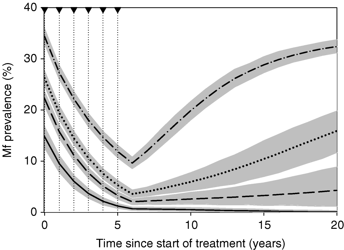
To investigate the behaviour of the model, we simulated the impact of a 6-year mass treatment programme on trends in mf prevalence. In our default simulations, we performed four series of 500 repeated runs, using the parameter values that were derived in the current study. The four series only differed with respect to the assumed biting rate (mbr=500, 750, 1000 or 2000). Assumptions about treatment are given in Table 3. In view of the large uncertainty about the effects of drug treatment on adult worms, we do not cxlaim to simulate a specific treatment regimen. Yet, the chosen parameters are in the range of ‘guesstimates’ for existing antifilarial drugs and drug combinations (see Stolk et al. (Reference Stolk, De Vlas and Habbema2005) for a discussion of available evidence). Each simulation run starts with a burn-in period and the resulting endemic equilibrium situation is taken as pre-treatment, time 0, situation. At time 0, the first treatment is provided and subsequent treatments are given with one-year intervals. The population is followed for 20 years after the start of treatment, via yearly epidemiological surveys. In years 0, 1, 2, 3, 4, and 5, the epidemiological surveys just precede the treatment. The results per series of runs were summarized by calculating the average mf prevalence at each survey, together with the 5th to 95th percentile range.
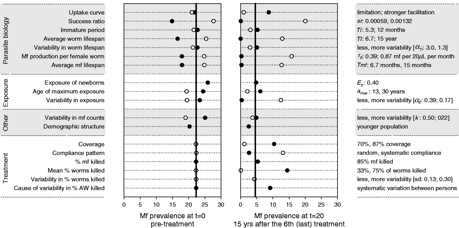
In a univariate sensitivity analysis, we assessed how the projected trends changed under other model parameter assumptions. With the mbr fixed at 750 bites per person per month, we performed new series of 500 repeated runs each. In each series, one of the model assumptions was assigned a different value from that in the default parameterisation; all other parameters kept their nominal value. Alternative values were usually chosen by multiplying the nominal value by 2/3 or 3/2 (or, if the nominal value of a proportion p was >50%, by multiplying (100−p) by these factors). For nominal proportions of 0% or 100% we chose alternative values that were still considered realistic: we used 0·40 as alternative value for relative exposure at birth E 0 (0 in the default model) and 85% as alternative value for the fraction mf killed per treatment (100% in the default model). Other parameters were treated in a more qualitative manner. The demographic parameters were changed as a group, to simulate a younger population with somewhat higher fertility rates and higher mortality rates in adults (representing the lowest income countries in sub-Saharan Africa). The uptake curve was replaced by other curves with weaker or stronger density dependence, corresponding to the confidence interval around the density-dependence parameter of the nominal equation (see Appendix 2). As alternative for the semi-systematic compliance pattern described above, we considered completely random or completely systematic compliance patterns. Lastly, as alternative for random variability in the fraction of worms killed by treatment, we considered a situation where treatment effects vary between but not within individuals. i.e. any variation in treatment effects is related to individual characteristics and some individuals always have a good response to treatment, while others always respond poorly.
RESULTS
Quantification of the model for Africa
The life table and fertility rates are shown in Fig. 2A and B (solid lines). With these parameters, the pyramidal-shaped structure of the African population is reasonably well approximated (Fig. 2C, grey bars).
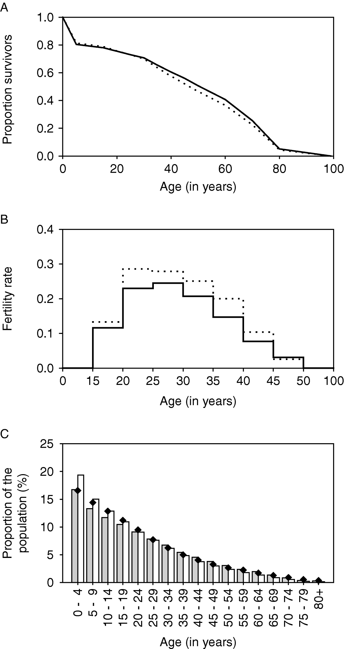
Fig. 2. Quantification of demographic parameters in LYMFASIM for modelling an African population. A: Survival curve, showing the survival probability as a function of age. B: Age-specific fertility rates, expressed as the mean number of births per female per year. C: Age-structure of the population that is simulated with the specified survival curve and fertility rates. The solid lines in A and B and the grey bars in C correspond to the default assumptions. The dotted lines and white bars give the alternative assumption which was used in the sensitivity analysis of simulating a younger population (with higher fertility and higher adult mortality rates). Black diamonds show published estimates of the population pyramid for the sub Saharan Africa population in 2002 (US Census Bureau, 2004).
Table 1 gives the values of other LYMFASIM parameters. The estimated value for parameter αE was 0·26, indicating that the probability distribution of exposure levels to mosquito bites is very skewed. The estimated value for the parameter sr was 0·00088.
With the estimated parameter values, LYMFASIM predictions fitted well to the epidemiological data from the African region (Fig. 3). Data about the relationship between the average mbr and overall mf prevalence were available from 11 locations in 4 countries (Table 2). As Fig. 3A illustrates, the models could simulate the entire range of observed mf prevalence levels, with values up to 40%, by varying the monthly biting rate parameter within a realistic range. The grey-shaded area in Fig. 3A indicates that most observations are within the range of possible model outcomes if model projections were subjected to the same sources of variation as the field data (see Materials and Methods section above for explanation). Fig. 3B shows that the model-predicted relation between mf prevalence and geometric mean mf intensity in the positives reflects the general pattern in the data from 9 locations in 4 studies (Brengues, Reference Brengues1975; Gyapong et al. Reference Gyapong, Badu, Adjei and Binka1993, Reference Gyapong, Omane-Badu and Webber1998; Boakye et al. Reference Boakye, Wilson, Appawu and Gyapong2004). The biting rate does not influence this relationship. Fig. 3C shows that the predicted age-prevalence pattern captures the main trend in locations with very low, low, intermediate or high overall mf prevalence. Data came from the 4 studies cited above, plus 7 other studies (McGregor, Hawking and Smith, Reference McGregor, Hawking and Smith1952; McFadzean, Reference McFadzean1954; Brengues, Subra and Bouchite, Reference Brengues, Subra and Bouchite1969; Juminer, Diallo and Diagne, Reference Juminer, Diallo and Diagne1971; Ripert et al. Reference Ripert, Eono, Eono, Tribouley, Appriou and Issoufa1982; Akogun, Reference Akogun1991; Anosike et al. Reference Anosike, Nwoke, Ajayi, Onwuliri, Okoro, Oku, Asor, Amajuoyi, Ikpeama, Ogbusu and Meribe2005). The mf prevalence increases with host age until a stable level is reached in adults. The biting rate only influences the average mf prevalence level and not the shape of the age-prevalence pattern.

Fig. 3. Comparison of model outcomes (based on nominal parameter values, Table 1) with data collated from literature. A: Relationship between monthly biting rate (mbr) and overall mf prevalence in the population. The solid line corresponds to model predictions, while the markers represent data presented in Table 2. The grey-shaded area shows the range of possible model outcomes if time-dependent or measurement error variation in the mbr and sampling variation in mf prevalence is taken into account (see Materials and Methods for further explanation). B: Relationship between observed mf prevalence and geometric mean mf intensity (GMI) in 20 μL of blood, based on age-specific data. The overlapping lines show the model-predicted relation for monthly biting rates of 500, 750, 1000 and 2000. The markers show the observations; observations that were made in different age groups from the same community share the same symbol. C: Relationship between mf prevalence and host age. The thin grey lines show the observed age-patterns in different communities. Different line types were used for villages with very low (dashed), low (dotted), intermediate (solid) or high (dot-dashed) overall mf prevalence. The thick black lines of the same type show the corresponding model predictions which were obtained with mbr of 400, 500, 750 and 2000 respectively.
Table 2. List of published studies that provide information about both the monthly biting rate and mf prevalence levels in African communities where Anopheles acts as main vector for lymphatic filariasis

Abbreviations: A.f.=Anopheles funestus; A.g.=Anopheles gambiae; C.q.=Culex quinquefasciatus; A.m.=Anopheles melas; MBR=monthly biting rate; n.r.=not reported.
* The average MBR is the mean biting rate over a period of 1 year, calculated as 1/12 * annual biting rate. The annual biting rate was estimated from landing catches, which were performed with regular intervals in a period of 12 months.
Default simulations and sensitivity analysis
Fig. 4 shows the results of our simulations using the nominal parameter values for areas with varying average mbr, with the treatment assumptions of Table 3. Mass treatment led to elimination in areas with low average biting rates (mbr=500), but to rapid recrudescence in areas with high biting rates (mbr=1000 or 2000). In areas with a biting rate of 750, the intervention reduced mf prevalence to low levels, but there was a tendency for slow recrudescence. (The grey area in Fig. 4 does not have the same interpretation as that of Fig. 3A. The range of possible outcomes in Fig. 4 is much narrower, because model outcomes are conditional on the assumed constant mbr value and because they ignore the non-simulated variability in mf prevalence measurement resulting from random sampling of the human population.)

Fig. 4. Model-predicted trends in mf prevalence during and after a 6-year mass treatment programme. Treatment takes place in the first 6 years of the simulation with the assumptions of Table 3. The dotted lines and arrowheads on the top-axis indicate the times of treatment. The thick lines show the average predicted trends for monthly biting rates of 500 (solid), 750 (dashed), 1000 (dotted) and 2000 (dot-dashed). The grey areas around each line indicate 5th to 95th percentile range of simulation results at each time. The results are based on 500 simulation runs. The trends are based on yearly measurements at t=0, 1, 2, …, 20; fluctuations between these time-points are not shown.
Table 3. Parameter assumptions about mass treatment and drug efficacy
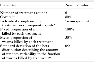
* See Appendix 1 for explanation.
† The default assumption is that this variation occurs randomly between treatments. The sensitivity analysis considered the alternative assumption that variation occurs systematically between individuals and that there is no variation within individuals.
Fig. 5 shows the results of the sensitivity analysis for a location with mbr=750. Four of the seven parasite biology parameters had a strong influence on the predicted mf prevalence levels before and after treatment, namely, the average worm lifespan, the rate of mf production per female worm, the average mf lifespan, and the success ratio of L3 larvae becoming established worms. While the strength and direction of density dependence in the uptake of infection by the mosquito barely influenced the pre-treatment mf prevalence, they had a very strong impact on the long-term impact of mass treatment and elimination prospects. Of the exposure-related parameters, the variability in exposure was most influential. Increased variability reduced the pre-treatment mf prevalence, but also led to faster recrudescence of infection after cessation of treatment. Higher values for the exposure of newborns and lower values of the age at which exposure achieves its maximum both resulted in a somewhat higher pre-treatment mf prevalence, but had little impact on the observed value after treatment. The variability in mf counts determined the probability of false-negative outcomes in mf counts, but not the underlying true level of infection. Its influence was largest in the pre-treatment situation. The mf prevalence was somewhat lower in a younger population. The impact of mass treatment was strongly reduced when we assumed lower coverage, systematic compliance, or a lower treatment effect on adult worms. The amount of variability in the latter effect was not very important, as long as the variation occurred at random. However, if drug efficacy varied systematically between persons (so that some people always respond poorly, while others might have a good response), the overall impact of mass treatment was substantially reduced.

Fig. 5. Sensitivity analysis: impact of changes in parameter values and other model assumptions on the predicted mf prevalence before and after an intervention with 6 yearly rounds of mass treatment. Post-treatment mf prevalence was measured in year 20, i.e. 15 years after the 6th (last) treatment round. The vertical black lines in each graph show the mf prevalence levels that were predicted by the model with nominal parameter values (Table 1). Markers show the results obtained under alternative assumptions. On the left side of the graph we provide descriptive labels for the parameters or assumptions concerned. On the right side of the graph we specify the alternative value for the parameters concerned, with the 1st value corresponding to the black bullet and the 2nd value (if available) to the white bullet. See Materials and Methods for considerations in choosing alternative values.
DISCUSSION
With the advancement of the Global Programme to Eliminate Lymphatic Filariasis, there is a growing demand for models that predict the long-term impact of control measures. We quantified the LYMFASIM simulation model (Plaisier et al. Reference Plaisier, Subramanian, Das, Souza, Lapa, Furtado, Van der Ploeg, Habbema and Van Oortmarssen1998) for use in African villages where Anopheles species act as main vectors, using a wide variety of reported data. Particular effort was made to test whether the model adequately captured general epidemiological patterns and differences between communities. By varying the average monthly biting rate within a realistic range (of about 100 to 4000 bites per person per month), we could simulate the entire range of observed mf prevalence levels, which ranged up to 40%. The relationship between mf prevalence and geometric mean mf intensity in the mf-positives, as well as the general age-patterns of mf prevalence matched with observations.
Model behaviour
We performed large numbers of simulations to examine whether the model behaved as expected and to provide insight into the influence of the many model parameters on the predictions. The model-predicted trends in mf prevalence during and after a 6-year mass treatment programme show that the elimination prospects are best in areas with low biting rates and low pre-treatment endemicity levels. The probability and rate of recrudescence after stopping treatment increase with higher biting rate and pre-treatment endemicity levels. These predictions are plausible, but remain to be validated against observed data (see below).
The sensitivity analysis provides much information about the effects of parameter values. Adjusting the success ratio, average worm burden, rate of mf production per female worm, and average mf lifespan resulted in major changes in the predicted pre-treatment mf prevalence, implying that the predictions are no longer in agreement with the data of Fig. 3A and that post-treatment predictions are not valid. This does not necessarily mean that the alternative parameters values are unrealistic: a better fit might be obtained by adjusting the fitted or other model parameters.
Our sensitivity analysis confirmed the importance of density dependence assumptions as reported by others (Duerr et al. Reference Duerr, Dietz and Eichner2005). We have paid particular attention to the quantification of the uptake curve, but some uncertainty remained about the strength of density dependence. Changing these assumptions had no impact on the predicted pre-treatment mf prevalence level or the goodness of fit in Fig. 3 (not shown). Yet, it strongly influenced the predicted post-treatment prevalence 20 years later. Thus, the remaining uncertainty about the strength of density dependence hinders accurate predictions of long-term effects of mass treatment. We also confirmed the importance of variability in exposure to mosquito bites for elimination prospects (Duerr et al. Reference Duerr, Dietz and Eichner2005). A higher degree of variability causes stronger aggregation in the distribution of the parasites over humans (some people harbouring many worms and others few or none); this increases the mating probability of worms, especially when worm numbers are low, and leads to higher risk and rates of recrudescence after stopping treatment. Differences between communities in the amount of variability result in variable elimination prospects (Dadzie et al. Reference Dadzie, Basáñez and Richards2004).
As previously shown, post-control predictions depend heavily on assumed coverage and compliance patterns (Plaisier et al. Reference Plaisier, Stolk, van Oortmarssen and Habbema2000; Stolk et al. Reference Stolk, Subramanian, Oortmarssen, Das and Habbema2003; Michael et al. Reference Michael, Malecela-Lazaro, Simonsen, Pedersen, Barker, Kumar and Kazura2004). This underlines the importance of assessing their actual values for evaluation of treatment programmes. The effects of treatment on adult worms are also very important, and uncertainty about this affects our ability to predict accurately post-treatment trends in infection.
Model validation
A strength of our validation approach is the comparison of the model predictions to data from a range of different communities. This helped to identify both the general pattern and realistic deviations. Deviations from the model-predicted average relationships can be large. See for example Fig. 3A. The model predicts a clear transmission threshold in the biting rate: if the average monthly biting rate drops below the value of 400, the basic reproduction ratio (R 0) becomes too low and the infection will die out (R 0<1). Such a threshold is theoretically plausible and our estimate was of the same order of magnitude as an earlier published estimate (Michael et al. Reference Michael, Malecela-Lazaro, Kabali, Snow and Kazura2006). However, the threshold pattern is not clearly visible in the data. Several reasons may be given as explanations for this. Firstly, the data are subject to measurement, sampling, or time-dependent variation. The latter is particularly relevant because trends and fluctuations in biting rates are not immediately reflected in mf prevalence levels. Because of these factors, the observations do not lie on the predicted curve, but can lie anywhere in the grey-shaded area of Fig. 3A. Secondly, local conditions can differ from the average conditions assumed in our model (e.g. with respect to variability in exposure, the age-structure of the population or anthropophagy of the local vector), leading to a different transmission threshold (Basáñez et al. Reference Basáñez, Collins, Porter, Little and Brandling-Bennett2002; Duerr et al. Reference Duerr, Dietz and Eichner2005).
The model predictions were only compared with cross-sectional data from treatment-naïve communities. A next step is to compare model predictions with longitudinal, post-treatment data. Evaluation data from the ongoing mass treatment programmes will be very helpful. Data collected during the first treatment years may not yet be very powerful for validation, because the model parameters are not uniquely identifiable. For example, effective mass treatment leads to a strong reduction in transmission. Uncertainty about treatment parameters (coverage, compliance, drug efficacy) precludes the accurate quantification of the remaining transmission. The most informative data for validating the underlying biological assumptions are probably those that are collected after cessation of prematurely interrupted or unsuccessful elimination campaigns: from the rate of recrudescence after cessation we can learn much more than from the rate of decline during mass treatment. Such data are available only for a few African villages (Meyrowitsch, Simonsen and Magesa, Reference Meyrowitsch, Simonsen and Magesa2004a, Reference Meyrowitsch, Simonsen and Magesab). It would be interesting to test the model against these data, but more data are needed to understand the general trends and possible deviations depending on local factors. Since the GPELF strives to achieve success in elimination programmes, such data will probably remain scarce for some time.
Uncertainty
One of the uncertain aspects in models for LF transmission is the role of acquired immunity. While strong acquired immunity was included in the Pondicherry model (Subramanian et al. Reference Subramanian, Stolk, Ramaiah, Plaisier, Krishnamoorthy, Van Oortmarssen, Amalraj, Habbema and Das2004), we found that evidence from the African continent is not consistent with this type of immunity as a strong regulatory factor of parasite population abundance (Stolk et al. Reference Stolk, Ramaiah, Van Oortmarssen, Das, Habbema and De Vlas2004). The difference between the Pondicherry and Africa model is somewhat unsatisfactory: it is rather unlikely that this mechanism plays a role in one region, but not in another. The new challenge is to define whether a model without acquired immunity can explain the observed patterns from Pondicherry if we take account of specific local conditions. In our earlier paper we discussed possible explanations (Stolk et al. Reference Stolk, Ramaiah, Van Oortmarssen, Das, Habbema and De Vlas2004).
The discussion about acquired immunity points at a more general problem in modelling LF transmission, i.e. our incomplete understanding of the transmission dynamics, the nature and magnitude of regulatory processes, and the effects of treatment. For example, we rejected the hypothesis that strong acquired immunity leads to a lower mf prevalence in elderly individuals, but we cannot exclude the operation of other regulatory immune processes (Woolhouse, Reference Woolhouse1992). Similarly, we lack knowledge about other factors that could influence the predictions, such as the occurrence of density dependence in the various processes of the parasite's life cycle (Duerr et al. Reference Duerr, Dietz and Eichner2005; Churcher, Filipe and Basáñez, Reference Churcher, Filipe and Basáñez2006), or the possibility that parasites become resistant against the antifilarial drugs (McCarthy, Reference McCarthy2005; Schwab et al. Reference Schwab, Boakye, Kyelem and Prichard2005, Reference Schwab, Churcher, Schwab, Basáñez and Prichard2007). We can also question the assumption that biological parameters such as the lifespan of adult worms and mf do not vary between locations. In the absence of evidence about these factors or data to validate assumptions, we kept the model parsimonious, trusting that the model captures the critical processes. Yet, this underlines the need to validate the model against longitudinal, post-treatment data, when they become available.
Application of the model
The model can be a useful tool for decision support in LF elimination programmes in the African region. For example, the model can help to determine the coverage and number of treatment rounds required for LF elimination under the different circumstances that occur in the African region using earlier published methods (Winnen et al. Reference Winnen, Plaisier, Alley, Nagelkerke, van Oortmarssen, Boatin and Habbema2002; Stolk et al. Reference Stolk, Subramanian, Oortmarssen, Das and Habbema2003). Further, detailed analysis of predicted trends after cessation of mass treatment can elucidate how the probability of achieving elimination depends on outcomes of epidemiological surveys in the end phase of treatment programmes and early years of follow-up. This will help to determine criteria for the cessation of mass treatment and to design surveillance schemes to monitor for possible recrudescence. Clearly, all predictions need to be accompanied by critical assessment of uncertainty. Making this uncertainty explicit can contribute to better and prudent decision-making.
Conclusion
In conclusion, we have developed a generic model for LF transmission by Anopheles mosquitoes in Africa, which captures the most important factors of LF dynamics and can easily be adjusted to specific circumstances by changing assumptions about exposure to mosquito bites. Its predictions are consistent with cross-sectional parasitological and entomological data. Although further validation against longitudinal, post-treatment data is required, the model already provides an important tool for decision-making in LF elimination programmes. The model can help to assess when ongoing elimination activities in African populations can be stopped and to design surveillance schemes. In view of the rapid expansion of the Global Programme to Eliminate Lymphatic Filariasis, these issues need to be addressed urgently.
ACKNOWLEDGEMENTS
We thank Dr Daniel Boakye for sharing data about the uptake of infection by Anopheles mosquitoes and for access to some unpublished data about time changes in annual biting rates. We thank Dr Johnny Gyapong for fruitful discussions about need for and potential applications of models for LF transmission in Africa in an early stage of the project. This investigation received financial support from the UNICEF/UNDP/World Bank/WHO Special Programme for Research and Training in Tropical Diseases (TDR).
APPENDIX 1. THE LYMFASIM SIMULATION MODEL
Simulation technique
LYMFASIM is based on the technique of stochastic microsimulation (Habbema et al. Reference Habbema, De Vlas, Plaisier and Van Oortmarssen1996). This technique is characterized by the simulation of individual life histories of fictitious persons, who in aggregate constitute the population of interest. The computer program tracks expected changes over time in the population composition and the relevant characteristics of each individual.
Model structure
The model simulates the demographic processes that drive population changes. Births and deaths are modelled as stochastic events in the life course of individuals. The expected number of newborns per time step depends on the number of females per age group and age-specific fertility rates. Random numbers define the realized number of newborns entering the population per time step. The age of death varies between individuals; it is defined as soon as a person enters the population by drawing a random variate from a life table. Immigration and emigration are not considered in the LYMFASIM model.
Each simulated individual has a number of characteristics, which define personal risk factors and behaviours that are relevant for transmission and control. Some of these characteristics are fixed, such as gender, attractiveness to mosquitoes, or willingness to comply with treatment. They are determined by randomly drawing a value from pre-specified probability distributions. Other characteristics can change during the course of a simulation, such as the age-dependent fertility rates and exposure to mosquitoes. Because of their personal characteristics, individuals may be predisposed to heavy or light infections. The infection status is the most important characteristic of human individuals. LYMFASIM simulates the transmission of parasites from person to person and tracks changes in the number of worms per individual.
A schematic representation of the variables and processes involved in transmission is provided in Fig. 1. Because LYMFASIM uses one-month time steps, all rates are expressed per month. The monthly transmission potential (mtp i) reflects the number of L3 larvae that are released to a person per month. On average, only a small proportion (called the success ratio, sr) of the released larvae will survive to develop further into adult worms; a chance process defines how many L3 larvae survive per month. The life course of surviving worms is simulated at individual worm level. Worms are immature during a period Ti and their average lifespan is Tl. The lifespan varies between worms according to a Weibull distribution with shape parameter αTl. We assume that all adult females are inseminated and produce microfilariae (mf), if at least one male worm is present in the human body. Parameter r 0 gives the mf production per female worm, expressed as the number of mf per month and per 20 μL of peripheral blood. Mf have a mean lifespan Tmf and their monthly survival is given by 1−1/Tmf. Mf are not simulated at the individual level; the model merely calculates the average mf density in the blood per individual (expressed in mf per 20 μL night finger prick blood). LYMFASIM has the option to include acquired immunity, which either reduces the probability of L3 larvae to develop into adult worm or reduces the mf output by female adult worms. Both mechanisms result in a lower mf count in elderly compared to young adults. As explained in the main text, acquired immunity is not included in the current model.
The ‘uptake curve’ (in this case given by a mathematical function with parameters a, b, and c) describes the deterministic relation between the mf density in the human blood of person i and the average number of L3 larvae that develop in a mosquito after feeding on that person (L3 i). The average number of L3 larvae taken up by mosquitoes is given by the weighted average of the uptake from all individuals, the weights reflecting the relative exposure of each individual to mosquito bites (E i, see below). This average number is multiplied by a factor v to calculate the average number of L3 larvae that is released per bite, ![]() . The factor v accounts for the proportion of L3 that is lost due to mosquito death and the proportion of L3 that does not leave the mosquito when it bites.
. The factor v accounts for the proportion of L3 that is lost due to mosquito death and the proportion of L3 that does not leave the mosquito when it bites.
The relative exposure of an individual (E i) indicates how many mosquito bites a person gets per month. It is expressed as a fraction of the average number of mosquito bites received per adult male per month (monthly biting rate, mbr). LYMFASIM accounts for age (and optional sex) variation in exposure and random variation in individuals' attractiveness for mosquitoes. Here we adopt the common assumption that exposure increases with body surface during growth in childhood and stabilizes in adults (Duerr et al. Reference Duerr, Dietz and Eichner2005; Smith et al. Reference Smith, Maire, Dietz, Killeen, Vounatsou, Molineaux and Tanner2006). We approximate this by a linear increase in relative exposure from E 0 at birth to the adult (maximum) level that is achieved at age a max. The random, not age-related variability in exposure is described by a gamma distribution with shape parameter αE and mean 1. An individual's relative exposure does not only determine his/her contribution to the mean L3-load of mosquitoes, but also the number of L3-larvae received: the monthly transmission potential (mtp i) is calculated as the mean number of L3 larvae released per mosquito bite (![]() , see above) multiplied by the mbr and the individual's relative exposure (E i). We assume that the mbr is constant over time, ignoring seasonal variation and other time trends.
, see above) multiplied by the mbr and the individual's relative exposure (E i). We assume that the mbr is constant over time, ignoring seasonal variation and other time trends.
Control strategies
To simulate the impact of mass drug administration, the user must specify the exact moments of treatment (year, month), the drug or administration regimen applied with its efficacy, the fraction of people treated per round (coverage), and the compliance pattern.
The three main effects of treatment are: (1) a fraction of adult worms is killed; (2) a fraction of female adult worms is permanently sterilized (i.e. they stop producing mf); and (3) a fraction of mf is killed. The fraction of parasites affected can be constant or can vary according to a chosen probability distribution function. In addition, for each of the three mechanisms, the user may specify a fraction of treated patients with no or full effect of treatment (i.e. the fraction of parasites affected is respectively 0 or 1). All stochastic variables related to the effects of treatment are by default assumed to be independent and to be generated for each person at each treatment. As an alternative, the treatment efficacy can be attributed as a fixed characteristic to an individual, who in that case always responds in the same way to treatment. Temporal reductions in the mf production can also be simulated (Plaisier et al. Reference Plaisier, Subramanian, Das, Souza, Lapa, Furtado, Van der Ploeg, Habbema and Van Oortmarssen1998), but these are not included here.
The compliance pattern describes the tendency of persons to participate in repeated treatment rounds. In case of random compliance, all individuals have the same probability to be treated (equal to the fraction covered). In case of systematic compliance, each person in the population is characterized by an invariable compliance factor (a random number between 0 and 1), which results in a treatment probability of either 1 (for compliance factor⩽coverage) or 0 (for compliance factor>coverage). Consequently, if coverage is constant over time, some individuals will always be treated while the remaining persons are never treated. In the case of semi-systematic compliance pattern, the compliance factor indicates a person's tendency to participate. Random numbers define whether an individual is actually treated or not. The latter pattern is presumably most realistic (Plaisier et al. Reference Plaisier, Stolk, van Oortmarssen and Habbema2000).
LYMFASIM also allows the simulation of selective treatment. In that case, treatment is only provided to those persons who were Mf positive in the most recent survey (which may take place in the same month as treatment, see below). Coverage and compliance play no role. Vector control can be modelled as a percentage reduction of the monthly biting rate during a specified period. The number of such periods, their duration and the reduction in monthly biting rate can be chosen.
Model output
At chosen times surveys can be simulated to determine the mf counts for all individuals in the population. We assume that this is done by microscopic examination of a 20 μL night blood smear. The counts are variable and are assumed to follow a negative binomial distribution with clumping factor k and the simulated mf density as mean expected outcome. The results can be summarized by different population-level indicators of infection: the mf prevalence, the geometric or arithmetic mean number of mf per smear, or the frequency distribution of mf counts in the population. Survey results can be tabulated by age group and gender.
Running the model
The program starts by creating an initial population, with specified size and age distribution. At the start of the simulation, some people are infected via some external force of infection. The model simulates how the population develops and how the infection level and other individual characteristics change in each one-month time step. To reach an endemic equilibrium situation and a stable age structure of the population, a simulation must generally cover a period of many decades. This is called a ‘burn-in’ period. Since the characteristics of persons are determined by chance or change as a result of stochastic processes, the result of one simulation run represents only one of many possible outcomes. Repeated runs will give slightly different results. The variability between runs reflects natural variation in real world populations, conditional on the appropriateness of the model structure. Simulations always have to be repeated to estimate the mean outcome and gain an insight into variability.
APPENDIX 2. QUANTIFYING THE UPTAKE CURVE FOR ANOPHELES
Methods
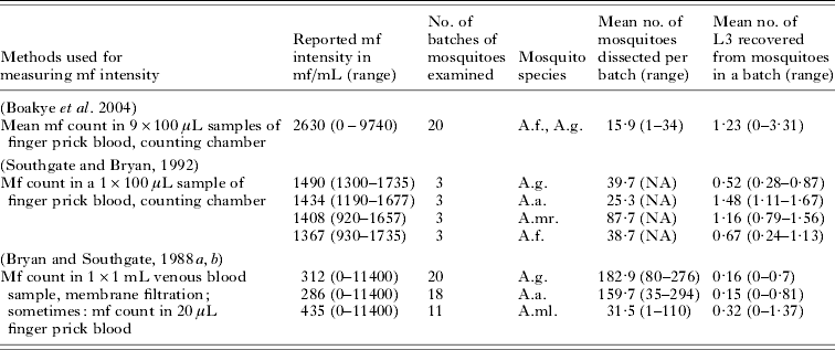
The uptake curve describes the relationship between mf density in the human blood and the number of L3 larvae developing in mosquitoes after feeding. To quantify this curve for Anopheles, we analyzed data about the average number of L3 larvae developing in a batch of mosquitoes that fed on an infected human with known mf density. Raw data were available from a field study in Ghana (Boakye et al. Reference Boakye, Wilson, Appawu and Gyapong2004). The few available data from published feeding experiments were also used (Bryan and Southgate, Reference Bryan and Southgate1988a, Reference Bryan and Southgateb; Southgate and Bryan, Reference Southgate and Bryan1992). Summary information of the different studies is provided in Table 4.
Table 4. Summary information about the data used for quantifying the vector uptake curve for Anopheles mosquitoes

Abbreviations: A.f.=Anopheles funestus; A.g.=Anopheles gambiae; A.a.=Anopheles arabiensis; A.mr.=Anopheles merus; A.ml.=Anopheles melas; mf=microfilariae.
To enable combined analysis of the data from different studies, we first standardized the mf counts to the expected count in a 20 μL finger prick blood smear. When reported mf counts were based on ⩽100 μL finger prick blood, we only applied a correction for volume. To transform mf count in 1 mL venous blood to corresponding count in 20 μl finger prick blood, we used the relationship that was derived by Snow and Michael (Reference Snow and Michael2002) : y=0·037x+0·1449x 2−0·0309, where: y=log10 (Mf count in 20 μL blood+1), x=log10 (Mf count in 1 ml blood+1).
Subsequently, we quantified the relationship between the standardized mf count in the human blood (mf per 20 μL) and the mean number of L3 developing in mosquitoes after feeding, by fitting equation 1 to the data.
with L3=the average number of L3 larvae developing in mosquitoes; M=the mf density in human blood as counted in a 20 μL night blood smear; a=the maximum number of L3 larvae that can develop in mosquitoes; b=1/scale; c=power-parameter. Depending on the value of the parameter c, this curve takes a saturating (c<1) or sigmoid form (c>1). The latter is suitable for describing ‘facilitation’ in the mf uptake and development, which is assumed for Anopheles: the number of L3 developing in mosquitoes initially increases more than proportional with the mf density in the human blood, but at higher densities limiting mechanisms get the upper hand so that saturation occurs (Southgate and Bryan, Reference Southgate and Bryan1992; Duerr et al. Reference Duerr, Dietz and Eichner2005).
Using the non-linear regression procedure (PROC NLIN) in SAS (v8.2), we estimated the values of parameters a, b and c with the least squares method. Observations were weighed for the number of mosquitoes examined. The weights (W i) were calculated as:
with x i the number of mosquitoes examined for observation i, and n the total number of observations included in the analysis. To prevent exclusion of observations with zero mf counts, we replaced the zeros by half the detection limit (with the detection limit being calculated as 1/(total blood volume examined in μL)∗20 μL).
Likelihood-based confidence intervals were calculated for parameter c (Kalbfleish, 1979). Confidence boundaries for this parameter were derived iteratively, by searching for the highest and lowest possible value that did not give a significantly worse fit to the data as assessed via the sum of squared errors (SSE). The maximum acceptable SSE (corresponding to the boundaries of the 95% confidence interval for parameter c) is given by SSEopt+3·84∗ scale, with the scale calculated as the sum of squared errors of the optimized model divided by the corresponding degrees of freedom (SSEopt/d.f.).
Results
The observations and estimated curves are shown in Fig. 6. There were 81 observations in total. The number of mosquitoes on which observations were based varied widely, from 1 to 294. Point estimates of the parameters of equation 1 were: a=1·67, b=0·027, and c=1·51. The solid line in Fig. 6 shows the shape of the uptake curve. The value of c>1 gives the curve a sigmoid shape, indicating that there is facilitation in the relationship between mf density in the human blood and the L3 yield per mf. However, the data used for estimation were highly variable and some uncertainty remains about the strength of density dependence. The dotted and dashed lines correspond to the upper and lower boundaries of the 95% confidence interval for the parameter c, respectively resulting in curves with weaker facilitation (a=2·11, b=0·013, c=0·81) or stronger facilitation (a=1·40, b=0·036, c=2·72). Note that the dotted curve in fact shows limitation: the L3 yield per mf is highest at the lowest mf density and continuously declines with increasing mf density.
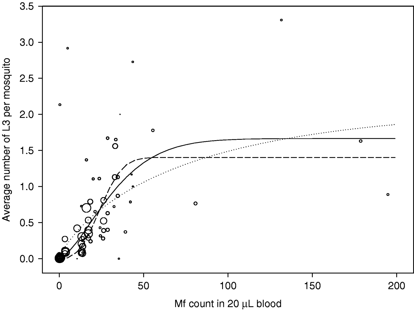
Fig. 6. Uptake curve, showing the relation between the mf count in human blood (mf per 20 μL of blood) and the average number of L3 developing per mosquito after a blood meal. Observations are shown as open circles and the circle size correlates to the number of mosquitoes examined. The solid line shows the best fitting curve; the dotted and dashed lines respectively give the curves that correspond to the lower and upper boundary for parameter c (the severity of density dependence).

