


Introduction
Many parasites and their hosts exhibit circadian rhythms that influence processes such as transmission, pathology and life cycle evolution (Mouahid et al. Reference Mouahid, Idris, Verneau, Théron and Shaban2012; Khan et al. Reference Khan, Dutta, Das, Pathak, Sarmah, Hussain and Mahanta2015; Théron, Reference Théron2015). Predictable cycles in the activity or habitat use of hosts offer an opportunity for parasites to increase the probability of successful infection (Aoki et al. Reference Aoki, Fujimaki and Isao2011; Théron, Reference Théron2015). Within human hosts, for instance, microfilariae of nematodes such as Wuchereria bancrofti, Brugia malayi and Loa loa, aggregate in peripheral blood vessels during periods of peak feeding by their arthropod vectors, presumably maximizing transmission to biting flies and mosquitoes (Hawking, Reference Hawking1967; Dreyer et al. Reference Dreyer, Pimentael, Medeiros, Béliz, Moura, Coutinho, Andrade, Rocha, Silva and Piessens1996; Aoki et al. Reference Aoki, Fujimaki and Isao2011; Craig and Scott, Reference Craig and Scott2014).
Parasites that depend on free-living infectious stages often exhibit circadian rhythms in their emergence from intermediate hosts. For instance, trematode parasites have frequently been used as a model for understanding parasite chronobiology (Lu et al. Reference Lu, Wang, Rudge, Donnelly, Fang and Websteer2009; Théron, Reference Théron2015; Soldánová et al. Reference Soldánová, Selbach and Sures2016). Trematodes use free-living infectious stages, such as eggs, miracidia and cercariae, to move among host species (Kuris and Lafferty, Reference Kuris and Lafferty1994; Parker et al. Reference Parker, Chubb, Ball and Roberts2003). Snails or other molluscs function as first intermediate hosts, from which mobile cercariae emerge and seek out a subsequent host species (Kuris and Lafferty, Reference Kuris and Lafferty1994; Parker et al. Reference Parker, Chubb, Ball and Roberts2003). Because cercariae are typically short-lived (<24 h), emergence patterns that increase the likelihood of host encounter are selectively favoured (Fried and Ponder, Reference Fried and Ponder2003; Karvonen et al. Reference Karvonen, Paukku, Valtonen and Hudson2003). For example, cercariae of human blood flukes (Schistosoma spp.), which infect approximately 200 million people worldwide (Fenwick, Reference Fenwick2012), emerge en masse from aquatic snails at times that parallel peak activity of local villagers (Silva et al. Reference Silva, Rotenberg, Bogéa, Favre and Pieri1995; Ahmed et al. Reference Ahmed, Ibrahim and Idris2006; Mintsa-Nguéma et al. Reference Mintsa-Nguéma, Mone, Ibikounle, Mengue-Ngou-Milama, Kombila and Mouahid2014). Intriguingly, parasite emergence patterns vary regionally in association with differences in village-specific behaviours as well as the role of alternative hosts (N'Goran et al. Reference N'Goran, Brémond, Sellin, Sellin and Théron1997; Lu et al. Reference Lu, Wang, Rudge, Donnelly, Fang and Websteer2009; Su et al. Reference Su, Zhou and Lu2013; Wang et al. Reference Wang, Lu, Guo, Li, Gao, Bian and Su2014). Su et al. (Reference Su, Zhou and Lu2013) reported that S. japonicum was more likely to emerge nocturnally in regions where rodents served as important reservoir hosts, whereas strains maintained in the laboratory emerge during the day. Similar host-specific timing effects have been demonstrated for trematode parasites of wildlife (Ahmed et al. Reference Ahmed, Ibrahim and Idris2006; Steinauer et al. Reference Steinauer, Mwangi, Maina, Kinuthia, Mutuku, Agola, Mungai, Mkoji and Loker2008; Faltynkova et al. Reference Faltynkova, Karvonen, Jyrkka and Valtonen2009; Komatsu et al. Reference Komatsu, Daisuke, Paller and Uga2014). Although the precise mechanisms controlling trematode circadian behaviours remain conjectural, environmental cues such as light availability, temperature, salinity and water pressure have been demonstrated to influence cercariae release from snails (Valle et al. Reference Valle, Pellegrino and Alvarenga1973; Williams et al. Reference Williams, Wessels and Gilbertson1984; Mouritsen, Reference Mouritsen2002; Sulieman et al. Reference Sulieman, Pengskul and Guo2013; Paull and Johnson, Reference Paull and Johnson2014; Wang et al. Reference Wang, Zhu, Ge, Yang, Huang, Huang, Zhuge and Lu2015).
A persistent challenge in the study of circadian rhythms involves selection of the appropriate analytical approaches. A commonly applied class of analyses is circular statistics, which involve observations of directional vectors around a unit circle (Su et al. Reference Su, Zhou and Lu2013; Théron, Reference Théron2015). While circular statistics recognize the continuity of temporal data, their application to parasitological circadian rhythms is challenging for several reasons. Assigning each parasite to a specific angle assumes they are completely independent observations, even when dealing with pulses of parasites that emerge from a host within the same temporal window. Circular statistics also tend to weight parasite species that produce large numbers of infectious stages more heavily. Moreover, null data (times when parasites are not released) are ignored, despite their clear biological significance to circadian patterns. A more suitable approach for parasite circadian rhythms is therefore cosinor analysis, which involves modelling temporal data with cosine functions to identify the rhythm-adjusted mean value [Midline Estimate Statistic of Rhythm (MESOR)], peak emergence values (amplitude) and the time at which peak values occur (acrophase) (Refinetti et al. Reference Refinetti, Cornelissen and Halberg2007; Cornelissen, Reference Cornelissen2014). Nonetheless, while numerous statistical programs and packages can implement cosinor regression (e.g. Lee Gierke et al. Reference Lee Gierke, Cornelissen and Lindgren2013; Barnett et al. Reference Barnett, Baker and Dobson2014; Sachs, Reference Sachs2014; Revelle, Reference Revelle2016), these options vary considerably in features and flexibility. While parasitological data often follow a Poisson or negative binomial distribution (Greene, Reference Greene2008), most analytical options assume a Gaussian distribution of the response, which may be difficult to approximate even following transformation. Similarly, because observations often come from multiple individual hosts or treatments, it is frequently necessary to include both covariates (e.g. experimental condition) as well as grouping terms (e.g. random intercept terms for the identity of a specific host or trial).
In the current study, we extend a generalized linear mixed modelling (GLMM) framework to cosinor analyses and then apply this approach to evaluate the circadian rhythms of eight trematode species from freshwater pond ecosystems. GLMMs allow for incorporation of different error distributions, such as binomial (e.g. infected vs uninfected), Poisson (e.g. count data with or without an offset term to account for varying sampling areas) and negative binomial distributions, which often better approximate the overdispersed counts inherent to parasite infection (Shaw et al. Reference Shaw, Grenfell and Dobson1998; Bolker et al. Reference Bolker, Brooks, Clark, Geange, Poulsen, Stevens and White2009; Lee et al. Reference Lee, Han and Giuliano2012). Moreover, GLMMs include fixed as well as random effects (random intercept or slope terms), which help to fit hierarchically structured data and improve coefficient estimates. Thus, they recognize and allow for correlated observation to be included without introducing problems associated with pseudoreplication. By applying GLMMs to counts of cercariae collected over 24 h periods from multiple trematode species, we: (1) determined whether each parasite exhibited predictable, non-random circadian emergence patterns; (2) characterized the timing and magnitude of peak emergence (including comparison of single- and multiple cosinor models); and (3) used a simulation-based sensitivity analysis to compare the parameter estimates with the classical least-squares (LS) approach. We conclude by discussing future directions in parasite chronobiology with an emphasis on potential factors affecting the timing of cercariae release and their physiological mechanisms.
Materials and methods
Snail collection
During the summers of 2011, 2012 and 2016, we collected rams horn snails (Helisoma trivolvis) from pond ecosystems in the eastern San Francisco Bay region of California, USA, including Contra Costa, Alameda and Santa Clara counties. We collected snails by hand, through dipnet surveys and during seine hauls (see Johnson et al. Reference Johnson, Preston, Hoverman and Richgels2013). After collection, we acclimated snails to treated (UV-sterilized, carbon-filtered, dechlorinated) tapwater over the course of 6 h before placing snails individually into 50 mL centrifuge tubes. Tubes were checked every 3–6 h for free-swimming cercariae; when detected, cercariae were identified to morphotype using Schell (Reference Schell1985). Whenever possible, we supplemented this coarse-level identification to finer taxonomic resolution using primary literature, molecular analysis and experimental infections (Johnson, Reference Johnson1968; Kanev et al. Reference Kanev, Fried, Dimitrov and Radev1995; Johnson et al. Reference Johnson, Preston, Hoverman and Richgels2013). In total, we isolated 93 infected snails: 30 snails infected with Ribeiroia ondatrae (Cathaemasiidae), 25 with Echinostoma sp. (likely Echinostoma trivolvis, Echinostomatidae), 16 with Cephalogonimus sp. (Cephalogonimidae), three with Alaria marcianae (Diplostomatidae), three with Zygocotyle sp. (Paramphistomoidea), 11 with Australapatemon sp. (Diplostomatidae), two with an unidentified Echinostomatidae (magnacauda morphotype) and three with an unidentified Schistosomatidae (brevifurcate-apharyngeate morphotype) (see Table 1). Infected snails were maintained at 21 °C with a 14:10 day:light cycle to mimic summer conditions in the region. Snails were fed ad libitum a mixture of Tetramin™ (fish food), agar and calcium.
Table 1. Results of generalized linear mixed modelling approach to cosinor analysis of freshwater trematode cercariae collected in California

For each trematode species, we present the number of infected snails included in trials, the downstream second intermediate hosts used by that parasite and the cosinor parameter estimates for species with a non-random circadian rhythm (mean value ± 1 s.e.).
a Orlofske et al. Reference Orlofske, Jadin and Johnson2015.
b Davies and de Núñez, Reference Davies and de Núñez2012.
c Johnson, Reference Johnson1968.
d Núñez et al. Reference Núñez, Davies and Spatz2011.
e Abdul-Salam and Sreelatha, Reference Abdul-Salam and Sreelatha2004.
Circadian emergence patterns
Over the course of 93 trials, we quantified the number of cercariae released by each infected snail over 24 h in 2 h intervals. This assumes that the circadian rhythm of trematodes in emerging from snails is 24 h, consistent with the previous research; if the rhythm is longer than 24 h, however, this method would not capture it. We placed each snail individually into a 50 mL centrifuge tube; after 2 h, snails were carefully transferred to a new vial with clean water and the previous vial was labelled, capped and refrigerated (4 °C). This process was repeated every 2 h for 24 h. Trials followed a natural light:dark cycle (light from 6:00 to 20:00 h), during which snails were not fed. We counted released cercariae using an Olympus SZX10 stereodissection microscope (Olympus Corporation, Tokyo, Japan). Every effort was made to minimize disturbances to the snails or alteration of their environmental cues during the transfer process. When necessary to aid in cercariae counting, vials were left at 4 °C for 24 h to limit their swimming activity prior to counting.
Statistical analysis
To determine the rhythmicity of cercariae release, we implemented a single-component cosinor analysis (meaning only one emergence peak was analysed) within a GLMM framework. As outlined in Refinetti et al. (Reference Refinetti, Cornelissen and Halberg2007) and Cornelissen (Reference Cornelissen2014), the general equation for a single cosinor is given by:
 $$Y(t) = M + A\cos \left( {\displaystyle{{2\pi t} \over \tau} + \varphi} \right) + e(t)$$
Key parameters include the period, τ (24 h for circadian rhythms, which is assumed to be constant), the MESOR, M (which in this case is rhythm-adjusted mean number of cercariae released across all observations); the amplitude, A (effectively the peak emergence value above and beyond the MESOR); and the acrophase, φ (the time at which peak emergence occurs). Prior knowledge of the period is required for cosinor analysis and was limited to 24 h in the current study. This equation can be rewritten into a LS regression model using the trigonometric angle sum identity, simplifying the equation to:
 $$Y(t) = \; M + \beta x + \gamma z + e(t)$$
where β = A cos(φ), γ = −A sin(φ), x = cos(2πt/τ), z = sin (2πt/τ)
Once β and γ are determined through optimization techniques (i.e. LS, maximum likelihood), the acrophase and amplitude can be extracted using the equations:
 $$A = (\beta ^2 + \; \gamma ^2)^{1/2}$$
 $$\varphi = \arctan \left( { - \displaystyle{\gamma \over \beta}} \right) + K\pi $$
where K is an integer.
Cosinor analyses can include single or multiple component analyses (Cornelissen Reference Cornelissen2014). A multiple component analysis adds two or more cosine terms and takes the form
 $$\eqalign{Y(t) & = M + A_1\cos \left( {\displaystyle{{2\pi t} \over {\tau _1}} + \varphi _1} \right) + A_2\cos \left( {\displaystyle{{2\pi t} \over {\tau _2}} + \varphi _2} \right) + \cdots \cr & + e(t)}$$
which is simplified into
 $$Y(t) = \; M + \beta _1x_1 + \gamma _1z_1 + \beta _2x_2 + \gamma _2z_2 + \; \cdots + e(t)$$
Equations (3) and (4) from the above can be used to calculate acrophase and amplitude for each cosine line added. The benefit of adding multiple components is to account for the possibility of having multiple peaks in a circadian rhythm.
To incorporate the cosinor method into a GLMM framework, we used the R package ‘glmmADMB’ (Skaug et al. Reference Skaug, Fournier, Bolker, Magnusson and Nielsen2016) to build models of cercariae release per snail as a function of time. Our data were modelled as a negative binomial distribution with a log-link, although we compared among alternative distributions (e.g. Poisson and Gaussian) using the difference in the Akaike Information Criterion (delta AIC) (Burnham and Anderson, Reference Burnham and Anderson2004; Symonds and Moussalli, Reference Symonds and Moussalli2011). We also evaluated whether to include a zero-inflation term to account for ‘extra’ zeroes in the dataset beyond what would be expected with a Poisson or negative binomial distribution (Zuur et al. Reference Zuur, Leno, Walker, Saveliev and Smith2009). As fixed effects, we included both cosine and sine terms as functions of time, which we first converted into radians with equation (3). Parasite species identity was incorporated as both a main (fixed) effect and as an interaction effect with the sine and cosine terms, thereby allowing us to evaluate how parasite species affected the intercept term (here, the MESOR) as well as the amplitude and acrophase. We included host subject (i.e. the specific snail) as a random intercept term to account for the 12 non-independent observations from each snail; alternatively, we also tried adding an offset term of total parasites produced by each snail (log10-transformed), which similarly functioned to capture much of the among-snail variation. This inclusion allowed for variation in the MESOR values among snails infected with the same parasite while still harnessing the full dataset to estimate amplitude and acrophase (as opposed to running separate analyses for each individual snail, which both limits the power of the dataset to detect overall trends and inflates the number of statistical tests to be performed). Mathematically, the offset term transformed the response from the raw number of cercariae released per 2 h to the proportion released relative to the total released over 24 h.
Before extracting estimates of the MESOR, amplitude and acrophase from each model, the use of a negative binomial distribution required exponentiation of the model as follows:
 $$\ln (Y) = M + \beta x + \gamma z$$
which simplifies to
 $$\; Y(t) = e^Me^{\beta x}e^{\gamma z}\,\,{\rm or}\,\,Y(t) = e^Me^{A\cos \left( {(2\pi t/\tau ) + \varphi} \right)}$$
Equations (3) and (4) from above can be used to calculate the parameters into response units with a few adjustments:
 $$MESOR = e^M$$
 $$A = e^M(e^{{(\beta ^2 + \; \gamma ^2)}^{1/2}} - 1)$$
 With the multiplicative nature of exponential functions, the  $(e^{{(\beta ^2 + \; \gamma ^2)}^{1/2}} - 1)$ term represents the proportion by which the MESOR increased during peak release, as opposed to the addition of a constant. Here, the amplitude is defined as the increase in cercariae during peak emergence relative to the MESOR [equation (10)]. Because we used a GLMM framework, parameters were estimated using maximum-likelihood estimation (MLE) rather than LS. Since both amplitude and acrophase were calculated using equations with estimates β and γ, which each had their own error [equations (3) and (4)], we performed a Monte Carlo simulation to account for error propagation and calculate the standard errors of the MESOR, amplitude and acrophase. Error propagation is a problem that occurs when multiplying estimated values – each of which have their own error – to obtain desired parameters. The Monte Carlo simulation uses the variance–covariance matrix for each parameter estimate to randomly generate a distribution of 10 000 values, from which the mean estimate and its standard deviation are calculated (Farrance and Frenkel, Reference Farrance and Frenkel2014; Harding et al. Reference Harding, Tremblay and Cousineau2014). Finally, we tested residuals from each model for temporal autocorrelation using autocorrelation function plots and compared whether a single component or multiple component cosinor model offered a better fit to the data. Statistical significance was determined by a P value of <0.05 for the coefficient of the sin or cosine term. Significance for either term indicates a non-random rhythm in parasite emergence.
Model evaluation
To validate our methods, we conducted a simulation study to compare the effectiveness of using a generalized linear model (GLM) in comparison with classical LS regressions. We focused on the effect of using an alternative error distribution and did not include a simulation with random effects, hence the simple GLM model in the simulation study. In R 3.2.4 (R Core Team, 2016) we used the ‘rnbinom’ function to create random datasets using a range of ‘true’ values for each parameter (MESOR: range 2–200; amplitude: range 2–200; acrophase: range 0–24 h). For each parameter, we simulated 100 data points over the given range at 25 different combinations of the remaining two parameters for a total of 2500 simulated data points. From there, a GLM and a LS model were created using the ‘glm.nb’ function from package ‘MASS’ (Ripley et al. Reference Ripley, Venables, Bates, Hornik, Gebhardt and Firth2016) and the ‘lm’ function, respectively (R Core Team, 2016). The parameters were extracted from these models using the above equations, and Monte Carlo simulation techniques were used to obtain confidence intervals for the extracted parameters. For example, values for the acrophase were extracted from 100 simulated time points between 0 and 24 h for all pairwise combinations of MESOR with values 40, 80, 120, 160 and 200 and amplitude values of 40, 80, 120, 160 and 200 (see Fig. 1 and supplementary Fig. A.1–A.2). This process was completed for all three parameters: acrophase, MESOR and amplitude. These values were chosen to broadly encompass the range of values observed empirically among these parasites. To compare between the LS and GLM, we calculated the number of estimates that contained the true value within the confidence interval and the distance between the true and estimated value. We calculated the line of best-fit using the ‘lm’ function in R to determine the slope and intercept between the estimated and true values; the closer the slope is to 1 and the intercept to 0, the less biased the estimates are. To evaluate the effects of the negative binomial distribution parameter (θ) and sample size (N) on parameter estimates, we created two additional 100 point datasets using fixed values of 150 for MESOR, 100 for amplitude, and 12:00 for acrophase, while varying sample size between 1 and 100 and θ between 0.2 and 10.
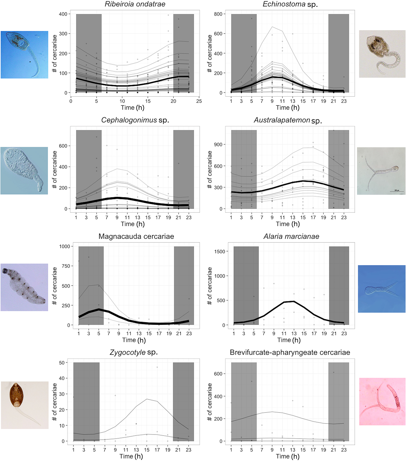
Fig. 1. Circadian rhythm of eight species of trematode parasites found in pond ecosystems. For each parasite, bold lines represent the overall, among-snail trend, faint grey lines are snail-specific estimates, and points are individual observations of cercariae counts within a 2 h period. The shaded vertical parts of the graph represent the hours the snails were in darkness (2000 to 0600). Images of each cercaria are presented on the outer margins of each plot.
Results
Circadian rhythms of aquatic trematodes
Our analysis strongly supported the existence of non-random, circadian rhythms in the emergence of trematode cercariae, but the patterns of release varied among species (Fig. 1). The best-fitting model incorporated a negative binomial distribution (dispersion parameter, θ = 104.71), fixed effects for parasite species, cosine and sine terms, and their interaction with parasite species (all P values for interactions were <0.05 except those for Zygocotyle sp. and brevifurcate-apharyngeate cercaria, which were >0.05), as well as a random intercept term for snail identity (380 point increase in AIC when random intercept removed, 102.8 point increase in AIC with offset instead of random intercept). Because the interaction terms were often significant, we subsequently performed a GLMM cosinor analyses with each of the parasite species individually and compared their parameter estimates. Non-random circadian rhythms – as evidenced by the presence of significant cosine or sine terms – were evident for R. ondatrae, Echinostoma sp., Cephalogonimus sp., A. marcianae, the magnacauda morhotype and Australapatemon spp., while no evidence of a consistent emergence pattern for Zygocotyle sp. or the brevifurcate-apharyngeate morphotype (although these two species also had among the lowest sample sizes) (Table 1 and Fig. 1). Residuals from the global model showed no evidence of temporal autocorrelation. The use of an offset for total cercariae released (instead of a random intercept term for snail identity) was favoured for all parasite species except R. ondatrae, for which the random intercept model performed better (delta AIC = 104.3), and A. marcianae, for which models were equivalent. Six snails that had <10 total cercariae emerge over the 24 h period were excluded from analyses.
Among trematode taxa, we observed considerable variation in all three of the cosinor parameters (Table 1). MESOR estimates ranged from 33 (A. marcianae) to 295 (magnacauda morphotype), with most values about 55 (Table 1); amplitudes ranged from 13 (R. ondatrae) to 386 (A. marcianae). Australapatemon sp. released the most cercariae per 24 h period (average 3062 ± 617 s.e.) followed by A. marcinae (average 2428 ± 763 s.e.), both of which significantly exceeded total cercariae counts by intermediate emergence patterns (Echinostoma sp., R. ondatrae and Cephalogonimus sp.) and the lowest levels of release associated with Zygocotyle sp. and magnacauda (GLM with negative binomial, McFadden's pseudo R 2 = 0.32, followed by Tukey's comparisons). For the subset of measured snails (n = 48), snail size had an additional, positive effect on the number of cercariae released per 24 h (coefficient for snail size = 0.14 ± 0.057, P = 0.014; McFadden's pseudo R 2 = 0.35). Among the diurnal species, Echinostoma sp. and Cephalogonimus sp. emerged earlier in the light cycle (estimated acrophase of 9:44 and 9:21, respectively), A. marcianae emerged around mid-day (12:11), and Australapatemon spp. emerged in the afternoon (~14:58). For nocturnal species, R. ondatrae and magnacauda emerged early in the dark phase (21:46) and late (5:10), respectively (although replication for magnacauda was low).
Model performance
Relative to the LS approach, the GLM method with a negative binomial distribution yielded more accurate estimates of the ‘true’ parameters from simulated datasets. For both MESOR and amplitude, the GLM approach improved accuracy (difference between estimated and true values) (Figs. 2 and 3, and Supplementary Figs. A.1–A.3). The average difference between the true and the estimated values of MESOR was 10.3 for GLM and 19.5 for LS estimates (t-test, P < 0.0001). With GLM, the 95% confidence intervals around the estimated MESOR were also 43.2% more likely than the LS approach to include the true values. Likewise, for amplitude, the difference between the estimated and true values averaged 34.9 using GLM and 37.4 for LS (t-test, P = 0.005). The confidence interval from the GLM was also 2× more likely to include the true amplitude relative to the LS model.

Fig. 2. A comparison of the ‘true’ and estimated values of the Amplitude parameter from the cosinor analysis between the traditional LS method and the GLM approach. The filled grey circles are the LS estimates, while the open circles are the GLM estimates. Each plot represents a different simulation with specified values of the MESOR (M) and the Acrophase (Acro). Each combination included 100 simulations drawn from a negative binomial distribution.

Fig. 3. Sensitivity of cosinor parameter estimates to variation in the negative binomial dispersion parameter (θ, which varied from 0 to 10). Each plot reflects the difference (estimated error) between the ‘true’ and estimated values from either LS or GLM for (A) MESOR, (B) Amplitude and (C) Acrophase. Dark circles and light triangles represent estimates from the GLM and LS approaches, respectively. The dashed horizontal line references the point at which the estimated and ‘true’ values are identical (difference of zero).
Estimation of the acrophase showed the least variation between methods, with an average difference between the true and estimated values of 0.88 h using the GLM and 0.92 h with LS (Figs. 2 and 3, and Supplementary Figs. A.1–A.3). Additionally, estimates for the acrophase clustered closest to the 1:1 line when the MESOR:amplitude ratio was low for both methods (A.1). The LS approach exhibited more bias in parameter estimates based on the best-fit lines, the slope and intercept for which should approach 1 and 0, respectively. The LS method tended to underestimate the amplitude as the true amplitude increased, with a slope of 0.47 compared with 0.97 for GLM. Conversely, LS overestimated the MESOR with an intercept of 24.0 and a slope of 0.93, while the GLM line had an intercept of 0.0 and a slope of 0.99 (Fig. 2 and Supplementary Fig. A.2). The GLMM models did not show the same biases for the acrophase parameter estimates (Fig. 2 and Supplementary Figs. A.1–A.2). Overall acrophase estimates from both methods become more variable with larger MESORs (Supplementary Fig. A.2). Increases in the negative binomial dispersion parameter (θ) or sample size (N) tended to decrease variance around the central tendency, suggesting that models will perform better with less extreme overdispersion (larger θ values) and larger datasets (Fig. 3 and Supplementary Fig. A.3).
Discussion
In the summer of 1920, William Cort observed that the number of cercariae released from freshwater snails varied dramatically among trematode species, in response to temperature, and even among individual snails (Cort, Reference Cort1922). Yet he further noted specific diurnal rhythms for each parasite, commenting that “…their constancy even over a considerable period is very striking.” Subsequent studies have consistently reported that many trematode species exhibit predictable circadian rhythms, in some cases showing population-level variation in timing that corresponds with local patterns of downstream host activity (Ahmed et al. Reference Ahmed, Ibrahim and Idris2006; Lu et al. Reference Lu, Wang, Rudge, Donnelly, Fang and Websteer2009; Théron, Reference Théron2015). However, an ongoing challenge has been matching the forms of data typically generated with analytical techniques that can appropriately answer researchers’ outlined questions. By using a cosinor analysis implemented within a generalized linear mixed modelling framework, we detected consistent circadian rhythms in six of eight tested species (R. ondatrae, Echinostoma sp., Cephalogonimus sp., Australapatemon spp., magnacauda morphotype and Alaria marciniae). Among the six species, chronotypes varied in all three parameters: acrophase (timing of peak parasite release, range: 5:10–21:46 h), amplitude (the increase from the MESOR of parasite release at the peak emergence, range: 13–386) and MESOR (range: 11–295). Both diurnal (Echinostoma sp., Cephalogonimus sp., Australapatemon spp. and A. marcianae) and nocturnal (R. ondatrae and magnacauda morphotype) emergence patterns were observed. No circadian rhythms were detected in Zygocotyle sp. or the brevifurcate-apharyngeate morphotype, although these two parasites had among the lowest sample sizes, so these results should be interpreted with caution.
Using a GLMM-based approach to cosinor analysis of circadian rhythms in the release of trematode infectious stages offers several benefits over previous methods. Data from parasitic circadian rhythm studies have key features that must be addressed: (1) the data are circular rather than linear, (2) the measurement of interest often involves count-type data with varying levels of overdispersion (Greene, Reference Greene2008), (3) observations are autocorrelated in space (host) or time, and (4) study designs often include a combination of fixed and random effects. Classical methods such as circular statistics (Su et al. Reference Su, Zhou and Lu2013; Théron, Reference Théron2015) – while well suited for the cyclical data inherent to biorhythms – do not track periods of parasite inactivity or facilitate concurrent testing of multiple covariates. More specialized approaches, such as the cosinor method (Favre et al. Reference Favre, Bogéa, Rotenberg, Silva and Pieri1997; Refinetti et al. Reference Refinetti, Cornelissen and Halberg2007), do not easily allow for hierarchical nesting in data (such as when the release of many parasites is recorded from replicate hosts) and generally assume a Gaussian error distribution. Integrating cosinor analysis into a GLMM framework helped address each of these issues, allowing for flexible error distributions (Poisson or negative binomial with zero-inflation), incorporation of multiple covariates (parasite species, sine and cosine terms, as well as their interactions with parasite identity), and the use of random-effects or grouping variables (in this case, individual snail identity to account for correlated observations from the same host). According to a simulation-based sensitivity analysis, implementation of a GLM framework outperformed a standard LS approach, yielding parameter estimates that were more accurate and more precise relative to the known range of parameters used in the simulation.
Application of this novel modelling approach also creates new opportunities to investigate the biological drivers underlying parasite circadian rhythms. Correspondence between parasite emergence time and peak host activity is often hypothesized to increase the likelihood of transmission into downstream hosts (Combes, Reference Combes2001; Lu et al. Reference Lu, Wang, Rudge, Donnelly, Fang and Websteer2009; Théron, Reference Théron2015). Our results provide mixed support for this hypothesis. While the nocturnal rhythm of R. ondatrae corresponds with the nocturnal activity patterns reported for some tadpoles (Oishi et al. Reference Oishi, Nagai, Harada, Naruse, Ohtani, Kawano and Tamotsu2004; Fraker, Reference Fraker2008), the trematodes Echinostoma sp., Cephalogonimus sp. and A. marcianae all exhibited diurnal rhythms for peak emergence, despite infecting the same secondary intermediate hosts (Table 1). Echinostoma sp. can also infect pulmonate snails as second intermediate hosts, which can exhibit both diurnal and nocturnal behaviour depending on their social interactions (Kavaliers, Reference Kavaliers1981; Keeler and Huffman, Reference Keeler, Huffman, Fried and Toledo2009). Cercariae of the Zygocotyle sp., which showed no consistent circadian rhythm in emergence, encyst directly on rocks or vegetation and may therefore be less constrained by host activity (Lang, Reference Lang1968), although other threats such as UVB exposure in shallow waters could select toward nocturnal emergence.
While more research on the activity patterns of the downstream hosts or substrates for these trematodes is necessary to critically test the ‘transmission hypothesis’, alternative explanations for the timing of emergence warrant further exploration, particularly in light of the broad variation in circadian rhythms among trematodes that all use similar intermediate hosts. Factors such as UV radiation, salinity, tidal cycles and the activity of non-host taxa may also contribute to the observed cycles of parasite emergence (Valle et al. Reference Valle, Pellegrino and Alvarenga1973; Williams et al. Reference Williams, Wessels and Gilbertson1984; Fingerut et al. Reference Fingerut, Zimmer and Zimmer2003; Sulieman et al. Reference Sulieman, Pengskul and Guo2013; Wang et al. Reference Wang, Zhu, Ge, Yang, Huang, Huang, Zhuge and Lu2015). For example, growing evidence suggests that cercariae are vulnerable to predation by aquatic taxa such as small fishes, cnidarians, molluscs and aquatic insect larvae (Thieltges et al. Reference Thieltges, Jensen and Poulin2008; Kaplan et al. Reference Kaplan, Rebhal, Lafferty and Kuris2009; Johnson et al. Reference Johnson, Dobson, Lafferty, Marcogliese, Memmott, Orlofske, Poulin and Thieltges2010; Orlofske et al. Reference Orlofske, Jadin, Preston and Johnson2012). In an examination of the digestive tracts of field caught estuarine fish, Kaplan et al. (Reference Kaplan, Rebhal, Lafferty and Kuris2009) detected cercariae in three of 61 fish, indicating that parasite consumption occurs in natural environments as well as under experimental conditions. Thus, emergence during periods of predator inactivity could increase the chance of successfully finding a host, whereas high overlap with predators could effectively suppress infection success. Orlofske et al. (Reference Orlofske, Jadin and Johnson2015) showed that while vertebrate and invertebrate predators were both effective at consuming cercariae in laboratory trials, the risk of consumption depended on traits of the parasite and the environmental context. Working with three of the same trematodes studied here, the authors found that species with larger cercariae – such as R. ondatrae – were especially vulnerable to small fishes and larval damselfly predators, whereas those with small (e.g. C. americanus) to intermediate (e.g. E. trivolvis) experienced correspondingly lower predation. However, predation risk further depended on light availability: trials conducted in the dark significantly reduced the number of cercariae consumed by visual predators, which is especially relevant for trematode species that naturally emerge at night (e.g. R. ondatrae) (Orlofske et al. Reference Orlofske, Jadin and Johnson2015).
Thus, despite the accumulating evidence in support of predictable biological rhythms for trematode cercariae emergence, many outstanding questions persist about the cues that induce release of infectious stages, how these patterns vary among species or populations, and even the mechanisms through which parasites track time, either directly or indirectly (Théron, Reference Théron2015). Such observations emphasize the need for more comparative research among trematode species or populations to evaluate variation in circadian rhythms and how they correlate with host usage, total release count and vulnerability to predation or physicochemical conditions, such as UVB exposure, salinity and water movements. Ultimately, development of flexible analytical techniques, such as those presented here, represent a useful prerequisite toward reliably characterizing parasite chronobiology and isolating the ecological and evolutionary factors underlying it. Moreover, while the current application was to parasitological data, the methods developed here can be extended to a wide range of systems with circadian data. Many datasets in chronobiology involve non-normally distributed data, including count data and binary outcomes, and it is often desirable to account for nested sources of non-independence, such as repeated observations on a subject, clustered locations in space, or animals in a particular group. Previous analytical methods often invoked multiple steps to first test for the presence of rhythmicity and then a second test to compare among subjects or between groups. The use of cosinor GLMM combines these into a single step and is thus suitable for testing circular data across biological as well as non-biological datasets.
Supplementary material
The supplementary material for this article can be found at https://doi.org/10.1017/S0031182017001706
Acknowledgements
We thank the following individuals for assistance in laboratory data collection: K. Leslie, J. Jenkins, T. Riepe, A. Oweimrin, S. Anderson and D. Rose. We also thank T. McDevitt-Galles and members of the field crews for snail collection. K. Prior, S. Reece and an anonymous reviewer gave input helping in revising the manuscript.
Financial support
This study was supported through funds from the National Science Foundation (grant no. DEB1149308), National Institutes of Health (grant no. R01GM109499) and the David and Lucile Packard Foundation.


